In the other approach, agents are risk averse and severance payments have non-trivial effects on welfare. 2Lazear's bonding critique argues that severance pay can be reversed through efficient agreements between workers and companies.
Match decision rules
Aggregate conditions
Equilibrium
The stock-flow equations for the different states of the economy (condition 7 in the definition above) can be derived from the description of the model in section 2.1. The numerical methodology and algorithm used to calculate a stationary equilibrium of the model are presented in Appendix A.1.
3 Calibration
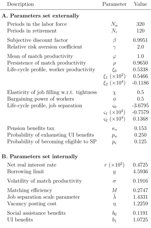
Parameters set externally
The shock standard deviation value, , is set below as part of the second step of the calibration exercise. We have set the elasticity of the probability of a job with respect to the tightness on the labor market at 0.50. As is standard (e.g. Bils et al. [2011]), we use the same parameter value for employee bargaining power in the base calibration.
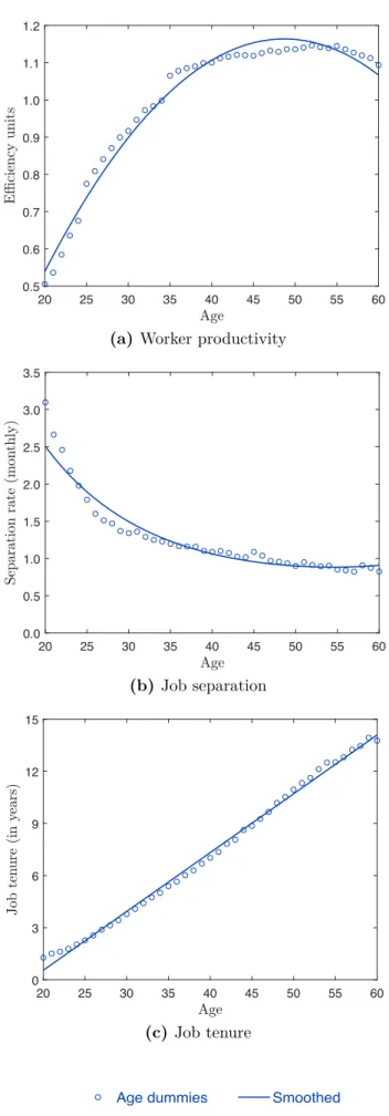
CPS data analyzed in Appendix B show that the job separation rate declines in a convex fashion over the life cycle. As the name suggests, ¯ allows scaling, or controlling, the relative importance of ⌧ to explain the post separation rate. The probability pu is set at 0.250 for UI benefits to expire after 26 weeks, consistent with U.S.
Finally, pe = 0.125, so workers become eligible for SP on average 1 year after employment.12 Of course, pe has no role in the baseline equilibrium, since SPs are set to zero.
Parameters set externally
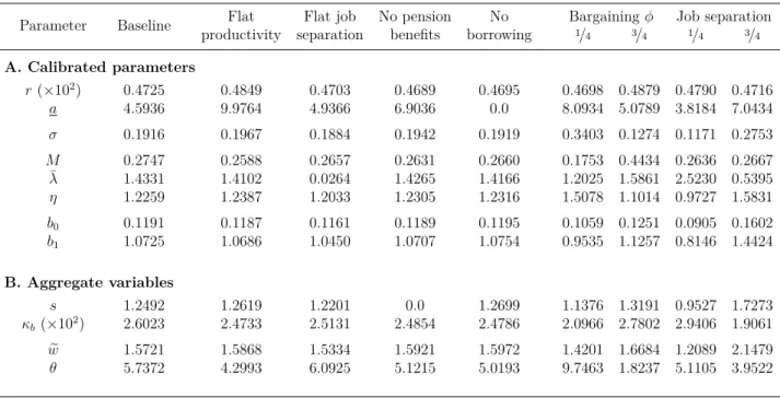
- Calibrated parameters
- Model outcomes
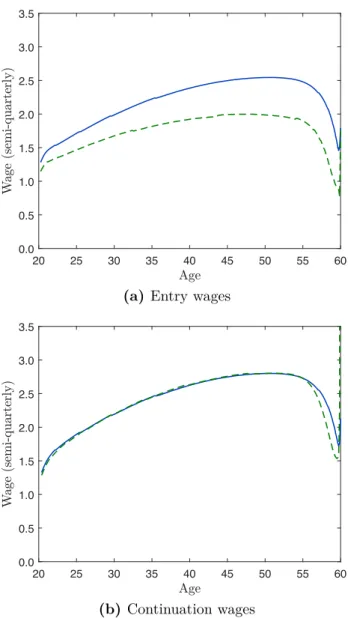
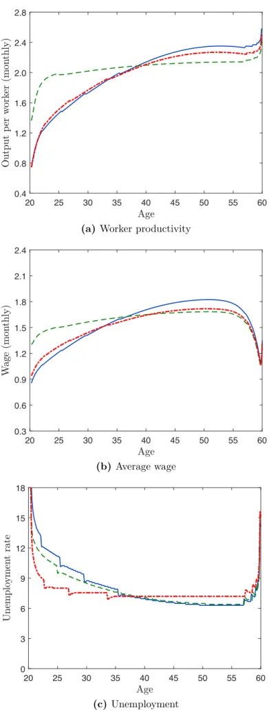
13However, when we consider a variant of the basic model, we recalibrate r in addition to the other parameters discussed in this subsection. As Table C1 in the appendix shows, each variant of the model has its own equilibrium value for the interest rate. The exogenous profile for worker productivity is the most instrumental in explaining why wages are lower at the beginning of working life.
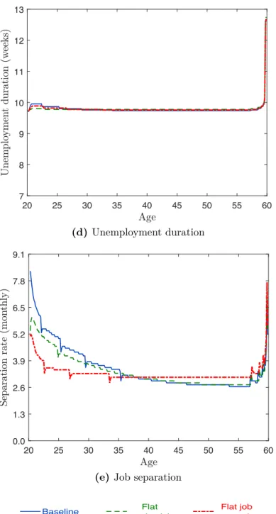
The decline in wages at the end of working life is too abrupt compared to the data, which is partly explained by the fact that retirement in the model is deterministic. As can be seen, unemployment declines rapidly at the beginning of the working life, which is in line with the data. In accordance with Figure B1b in the appendix, the job separation rate declines sharply at the beginning of the working life.
As can be seen, Plot 1e also shows a large increase in the separation rate at the end of the working life.
4 Quantitative analysis
Preliminaries
Figure 1b shows the life cycle profile of wages in the basic model and its variants. Although these characteristics are counterfactual, they are not essential to the results obtained in the following sections. While this feature is absent in the empirical behavior of the employment-to-unemployment probability, it is consistent with the behavior of the employment-to-nonparticipation probability (Choi et al. [2015]).
At the end of the data, unemployment is almost constant before age 45 and then starts to rise. In the sequel, we draw a comparison between welfare in steady-state equilibrium without SP and welfare in other economies. First, as we mentioned in subsection 3.2, we hold the interest rate fixed at the value calculated in the equilibrium without SP.
Second, since the complexity of the model precludes the calculation of the transition dynamics, we only consider steady-state equations.18 Note that the welfare criterion we use is fully justified in the context of such equations.
Changes in severance payments
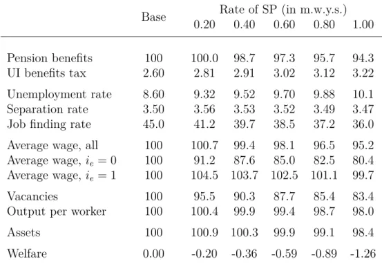
20However, for high levels of SP (such as those in Figure 2), this effect is offset by the decrease in the probability of finding a job. Subsequent wages are shown in the bottom graph of Figure 2, which we will discuss briefly. Alternatively, we can choose to set these variables to their value in the economy with SP.
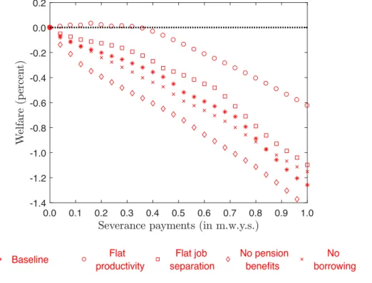
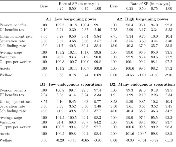
These two estimates show that the welfare loss resulting from differences in wage schemes is -0.54 percent and -0.98 percent, respectively. Compared to the number reported in the last column of Table 2, this suggests that between 43 and 78 percent of the welfare loss is caused by SP wage effects alone. One possible explanation is that, in the baseline model, young workers receive lower wages as they are less productive and more likely to leave the firm, and thus suffer more from the wage drift effects of SP.
In the four variants of the model, the wage shift effects remain the key mechanism for understanding the welfare consequences of severance payments.
Discussion
In this version of the model, workers have a much higher willingness to save, which is similar to the scenario considered by Alvarez and Veracierto [2001]. Yet the order of magnitude of the welfare figures remains similar to that of the baseline experiment.22 Finally, perhaps surprisingly, we find that setting the borrowing limit to zero has little to no effect on the welfare losses. He finds that the rate of wage growth has fallen relatively more in small firms, suggesting that employers in those firms have gained more bargaining power.
They estimate that for incumbent workers only 10% of the wage change can be attributed to the reform, whereas 50% of the wage increase for new hires comes from lower severance costs. In his study, Martins[2009] also assesses the impact of the reform on labor turnover and finds that the effects are not statistically significant. Focusing on the 1990 reform of the Italian labor market mentioned earlier, Kugler and Pica [2008] find that higher severance costs reduce employee turnover in small vs.
The fact that results often turn out to be nonsignificant in this literature suggests that most adjustments to SP occur through changes in wages.25.
5 Robustness checks
As can be seen, with lower bargaining power we find that SP can benefit workers, although welfare figures eventually decrease as we continue to increase the SP rate. For example, as can be seen by looking at the behavior of the average wage, the impact of SP on wages is significantly attenuated when the bargaining power of workers is lower. To rationalize these findings, note that tighter employment protection creates the classic barrier problem between firms and workers, and that increasing the bargaining power of workers exacerbates this issue.
We check the importance of the 'magnitude' of SP, by varying the relative importance of endogenous job separations. In subsection 4.2, we discussed the welfare implications of SP in various variants of the model that focused on aspects related to the life cycle or to preventive savings. The effects of SP on equilibrium allocations and wages (in addition to the welfare effects) in these experiments are reported in Table C2 of the appendix.
We also examined how these four variants perform when workers' bargaining power is switched to lower or higher values, or when we change ¯ to focus on a different share of endogenous job separations.
6 Conclusion
Specifically, the calibration in panel B1 of Table 3 implies that endogenous separations account for 25 percent of all separations of duties, while in panel B2 the corresponding figure is 75 percent (vs. 50 percent in the base calibration). To understand this, we need to consider that if we change the scope of the SP, we also need to change the exogenous risk of unemployment to match the job separation target. The uncertainty regarding the share of job separations that could be influenced by SP (see footnote 14) therefore does not appear to be decisive for our results.
Finally, we investigated the effects of using SP for exogenous workplace separations (in addition to endogenous separations). 2012] suggest that the replacement rate of unemployment benefits should decrease for the unemployed who are about to retire due to moral hazard. Michelacci and Ruffo [2015] also find that unemployment benefits should decline with age and argue that these benefits are more valuable to young workers who have few savings.
It would be very interesting to re-examine these questions – in isolation, and also addressing the issue of the joint design of unemployment benefits and severance payments – through the lens of our model.
Cyclical and secular behavior of labor input: Comparing efficiency units and labor hours. The impact of layoff restrictions on labor market equilibrium in the presence of workplace search.
Appendices
A Model appendix
Numerical algorithm 26
Both who(y, a,⌧) and who(y, a,⌧) are the solution to fixed-point problems: a guess on the reservation wage yields an asset holding decision that affects the continuation value and thus the reservation wage . In step 5, when T⌧ >0, knowledge of U1(a,⌧)above the upper bound of the asset grid is required. In practice, we see that regressing U1(.,⌧) against a second-order polynomial of a, based on the last top lattice points, produces an R-square that is indistinguishable from 1 to at least 4 decimal places .
The interest rate
B Data appendix
To measure worker productivity, we combine data from the CPS cohort samples for the 1995–2015 outgoing rotation. Like Hansen [1993], we define labor efficiency units as the ratio of a worker's hourly rate to the sample mean hourly rate. The rate of separation from employment is defined as the probability of transition from employment to unemployment.
The data used to study employment relationships come from the CPS supplements on occupational mobility and employment relationships. Let qa,t denote, for persons of age a observed in period t, a variable that interests us, e.g. the worker's productivity, the degree of separation or the length of employment. Dt) is a full set of age (respectively time) dummies and a,t is the residual of the regression.
The parametric life cycle profiles (indicated by a solid line in each graph of Figure B1) are described in sections 3.2 and 4.1 of the main text.
C Additional results
No pension benefits D. No borrowing