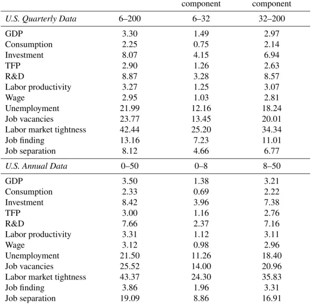
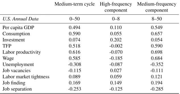
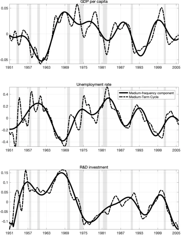
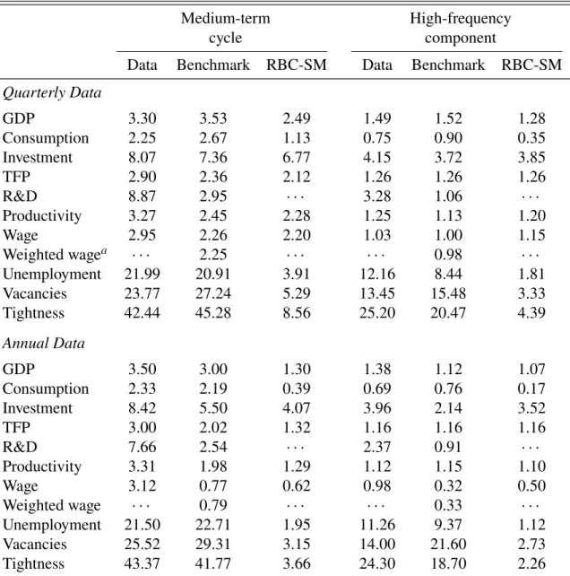
Labor market variables are twice as volatile in the medium-term frequencies than in the cyclical frequencies. Figure 1 provides a first look at the medium-term cycle in three key variables in the United States. We plot data for the medium-term cycle and its high-frequency component (business cycle).
3 The Model
- Final good sector
- Intermediate goods sector
- R&D sector
- Households
- Government
- Frictional labor market and wage determination in the final good sector
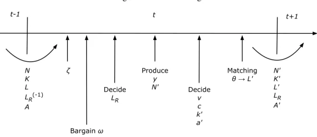
- Timing
- Equilibrium
- Balanced growth path
Denote𝑉 (𝑙 ,Ω) the value function of the final good producer who hired 𝑙 workers, 𝑣 the number of vacancies to be posted for the next period, and 𝜅 the parameter that determines per vacancy posting cost. Also let 𝛽Λ(Ω,Ω0) denote the firm's appropriate discount factor.8 The problem of the final good producer can be written recursively as. As will be seen later, this specification ensures the existence of a well-defined deterministic balanced growth path.9 The corresponding decision rules for the final good producer are functions.
Namely, one unit of variety𝑖can be produced at constant marginal cost𝜇 >0 units of the final good. Each intermediate good producer maximizes the value of expected discounted monopolistic profits by choosing the price of its output subject to the final demand schedule for the goods sector. The newly invented varieties become available for use as production inputs in the final goods sector in the following period.
We assume that the household is the residual claimant of the profits generated by firms in the intermediate and final goods sectors, (Π𝑖,Π𝑓). The labor market in the final goods sector is characterized by search and matching frictions. On the household side, workers may be employed in the final goods or R&D sector or unemployed and looking for work.
The investment determines the stock of physical capital and the amount of final goods for R&D input available for rent in the next period (𝐾0,𝐴0).
4 Calibration
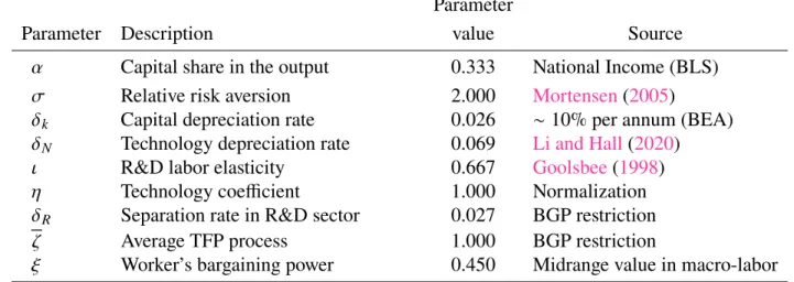
Baseline calibration
The gross growth rate of the innovation opportunity frontier along the balanced growth path is given by𝑔𝑁 =1−𝛿𝑁+𝜒(𝑙𝑅)𝜄(𝑎)1− 𝑔𝑁 with respect to𝑙𝑅. Using the balanced growth path constraints, the mean of the TFP shock process is set to one and the allocation rate in the R&D sector is set to 0.027. Finally, we specify the parameter governing worker bargaining power =0.45, which is near the middle of the range of values in the macroeconomic-labor literature.17.
The values of the remaining eleven parameters were set to enable the model to replicate selected empirical moments along the balanced growth path. We choose the value for the discount factor 𝛽 to match the annual long-term real interest rate of 5.0 percent with reference to the average annual return on the S&P500 index.18 The elasticity of the production function with respect to intermediate inputs corresponds to the investment-GDP ratio .19 The curvature parameter of. The targets for calibrating the persistence (𝜌𝜁) and volatility (𝜎𝜖 𝜁) of the AR(1) process governing the productivity shocks are the first-order autocorrelation and volatility of the high-frequency component of Fernald's (2014) TFP2014- series.
There are two potentially less standard aspects of our calibration that appear important for the quantitative implications of the model. Second, the calibration of the value of non-market activities to workers can have an important impact on the model's ability to amplify the effects of fluctuations on labor market quantities.
Alternative calibration
5 Results
Impulse response functions
A positive TFP shock raises the productivity of intermediate inputs, capital and labor in the final good production sector. In equilibrium, this leads to a greater quantity of each existing type of intermediate goods used as an input in the production of final goods, and to an increase in the price index of intermediate inputs. Note, however, that there is no immediate increase in the number of intermediate product types upon impact, as this mass is predetermined by the R&D efforts of the previous period.
Because the hiring of workers by the final good firms is also predetermined, the amount of labor input in the final good sector also remains unchanged on impact (panel 4). Nevertheless, the current employment opportunities create a higher surplus to be divided between the firms and workers, which is reflected in a higher wage rate in the final good sector (panel 5). This increases the expected future productivity of intermediate inputs, capital and labour, leading to an increase in the value of intermediate goods producer firms (panel 14), investment and future capital stock (panel 3), and the final good firms' incentives to fill job vacancies ( panel 8).
The higher discovery of new varieties of intermediate inputs further increases productivity in the final good sector in subsequent periods, triggering a strong feedback effect that leads to large and persistent responses of macroeconomic and labor variables to productivity fluctuations. In contrast, the variables in the RBC-SM model simply return to their original balanced growth path levels in the long run.

Medium-term cycles
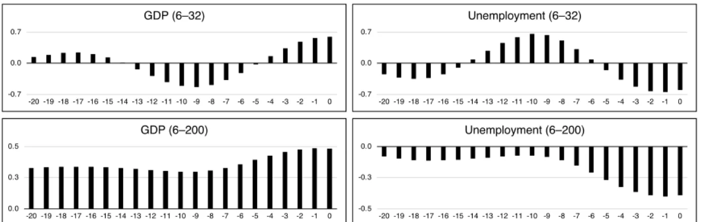
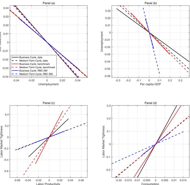
However, examining the autocorrelograms for GDP and unemployment in Figure 8 in more detail reveals that the medium-term cycle autocorrelation decays faster in the RBC-SM model than in the benchmark model. In terms of Okun's law (panel (b) of Figure 11), the benchmark model generates an elasticity of unemployment to GDP that is close to the elasticity observed in the real medium-term cycle data. In both models there is virtually no difference in the slope of the regression line for the medium-term cycle and for its high-frequency component.
The relationship between labor productivity and labor market tightness (Panel (c) of Figure 11) in the benchmark model implies a higher elasticity of tightness to productivity than in the data. However, the difference in the slope of the regression line between the medium-term cycle and its high-frequency component is in quantitative agreement with the real data. The RBC-SM model also fails to produce any significant difference in the value of this elasticity between the medium-term cycle and its high-frequency component.
In the regular RBC-SM model, there is a clear one-to-one relationship between labor productivity and labor market tightness. Finally, the benchmark model for the relationship between labor market tightness and consumption (panel (d) of Figure 11) implies an elasticity between the two variables close to that in real data, both in the medium term and in its high-frequency component .
6 Conclusion
Because the specialization of R&D labor involves quadratic adjustment costs and past discoveries permanently affect the value of future innovations, these effects affect the market for final goods more gradually, which translates into a lower correlation between labor productivity and tightness in the medium run cycle. Both models imply slightly higher correlation coefficients than those observed in the actual data for this relationship. Business cycle, data medium-term cycle, data business cycle, comparative medium-term cycle, comparative business cycle, RBC-SM medium-term cycle, RBC-SM.
Red lines correspond to the linear fit to the data simulated with the benchmark model. Blue lines correspond to linear fits in the data simulated with the RBC-SM model. Our results show that the expectations of the future evolution of productivity growth through innovation can significantly amplify and propagate the effects of current productivity shocks on the labor market variables.
Many questions remain to be answered by future research, particularly regarding the behavioral implications of labor market, innovation and education policies.
When can changes in expectations cause business cycle fluctuations in neoclassical settings?” Journal of Economic Theory. Business cycles, unemployment insurance and the calibration of matching models.” Journal of Economic Dynamics and Control. An Empirical Examination of the Procyclicality of R&D Investment and Innovation.” Review of Economics and Statistics.
Unemployment and Vacancy Fluctuations in the Matching Model: Inspecting the Mechanism.” Economic Quarterly, Federal Reserve Bank of Richmond. Estimating R&D Depreciation Rates: A Suggested Methodology and Preliminary Application.” Canadian Economic Review / Revue cana-dienne d'Economique. Look at the labor market and the real business cycle.” Journal of Monetary Economics.
Job Creation and Destruction in the Theory of Unemployment.” The overview of economic studies.
A Data
- GDP, consumption, and investment
- Total factor productivity
- Research and Development
- The labor market variables
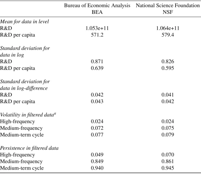
An alternative way to measure TFP in the model would be to recalculate TFP in the data using a capital measure that includes housing and durable goods. The R&D investment series is deflated using the R&D chain price index (code: Y694RG3Q086SBEA, http://fred.stlouisfed.org/ . series/Y694RG3Q086SBEA). While the BEA series measures the R&D investment, the NSF series measures the cost of R&D or R&D expenditure and is only available at an annual frequency.
Thus, BEA's measures of R&D investment are designed to capture the value of R&D, not current R&D costs, as in the NSF series. The Help Wanted Advertising Index and the Labor Force are quarterly averages drawn directly from the monthly series. As in den Haan and Kaltenbrunner (2009), the number of employees used to calculate the employment rate differs from the number of employees used to calculate labor productivity and wages.
In addition, in the calibration exercise we use statistics on the number of R&D scientists and engineers as reported by the NSF to measure the number of workers in the R&D sector (http: //www.nsf.gov/statistics/ industrial workforce). The number of R&D scientists and engineers indicates the total number of people employed domestically by R&D performing companies who were involved in scientific or engineering work at a level that required knowledge, either formally or by experience, of engineering or of the physical, biological, mathematical, statistical or computer sciences equivalent to at least that obtained by completing a 4-year college program with a major in one of those fields.
B Balanced growth path