Martin Magill was in charge of the theoretical analyzes and writing of the manuscript. The manuscript is included in the main text and reflects the major contribution I made to the collaborative research and writing of the manuscript.
Developing Computers for Science
New operating systems, programs that control many aspects of the hardware and software in a computer system, were being designed. Thanks to the release of the Apple-1 by Steve Wozniak and Steve Jobs, this decade also saw the rise of personal computers.
Computational Science in Biophysics
Molecular Dynamics Simulations
Specifically, in Chapter 3, MD simulations are used to study the movement of fluttering bacterial colonies. Finally, in Chapters 5–7, MD simulations are used to simulate the passage of particles through the slit-well microfluidic device known for its sorting capabilities.
Leveraging Deep Learning
Like deep learning in general, NNM is a computational technique whose potential continues to grow as a research tool for biophysics. In Chapter 6, the NNM is specifically implemented to resolve the electric potential and electric field in the microfluidic slitwell device.
Langevin Dynamics
Furthermore, the magnitude of the random force term depends on the properties of the fluid. The magnitude of the random force term also depends on the viscosity of the fluid.
Interactions
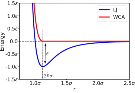
The repulsive regime of the LJ potential is used to model the excluded volume interaction, while the attractive regime models dipole-dipole forces. Thus, the LJ potential is typically modified in two ways to achieve the Weeks-Chandler-Anderson (WCA) potential (indicated in red in.
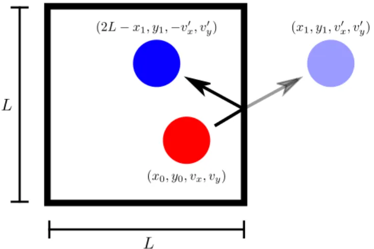
Boundary Conditions
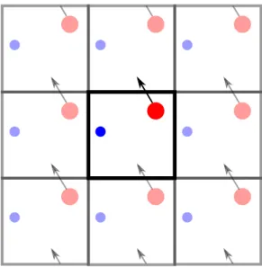
Alternatively, periodic BCs can be used to model an infinite system while still defining the simulation in a finite box. Periodic BCs can be viewed as the simulation box that repeats itself an infinite number of times (called frames) in all directions (as illustrated in Fig. 2.8).
Velocity Verlet and Numerical Integration
Simulation Software
GROMACS is designed to simulate Newtonian equations of motion for systems with hundreds to millions of particles. As a result, GROMACS is particularly suitable for simulating atomistic structures that tend to contain a large number of particles.
Deep Learning and Neural Networks
Supervised Learning
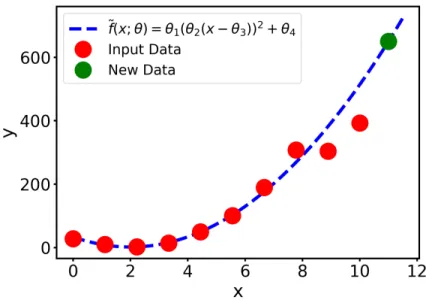
This trained function can then be used to predict output values for new data (represented by the green marker in Fig. 2.9) based on the relationship learned between x and f(x). Thus, a simple training algorithm such as linear regression can be used to find the parameters off˜(x;θ) that result in the best fit for the training data (x, f(x)).
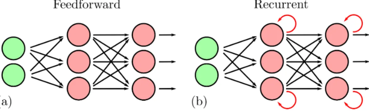
Forward Propagation
In general, the result is layers of a fully connected neural network of width w and depth d. To visualize the neural network equation, a schematic of a fully connected neural network with 2 hidden layers with 2 nodes is included in the figure.
Activation Functions
Cf. 2.27), a linear activation cannot be used in the hidden layers, because the neural network would be just a linear function. Thus, another role of the activation function is to introduce nonlinearity into the neural network.

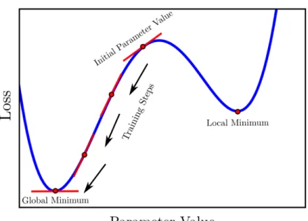
Gradient Based Learning
Similarly, the partial derivative of the loss function must be calculated for each weight and bias in the neural network. In fact, the term ∂L∂f˜ can be reused in the calculation of the gradient of any parameter in the neural network.
Hyperparameters
The formula for the capacity of a fully connected feedforward neural network of width w, depth and with a single input x is. The capacity of a neural network is an essential hyperparameter as it refers to the range/types of features that the neural network can approximate. A neural network with insufficient capacity may not be able to learn from the training data.
A high-capacity neural network, on the other hand, has the freedom to model more advanced types of features. Nevertheless, a neural network with too much capacity can be extremely slow to train and may memorize the training data to the point that it cannot generalize to new data.
Neural Network Method of Solving Differential Equations . 56
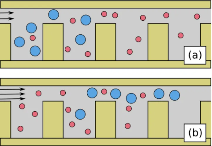
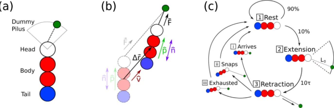
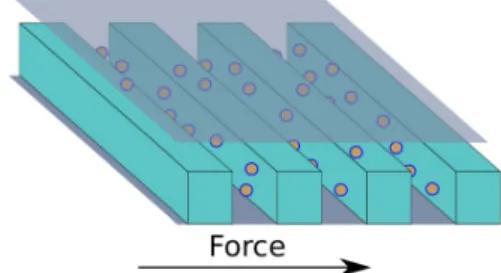
34;no data." This means that while traditional machine learning requires a large database of precomputed training data (ie, images, datasets, etc.), NNM does not. Many bacteria are modeled at the same time, only explicitly interacting with each other. via an excluded rebound volume (Chapter 2.1.2) in a quadratic domain with periodic boundary conditions (Chapter 2.1.3) as shown in Fig. 1] the properties of a solitary jerk are investigated to analyze the consequences of the motion cycle.
From t≈10−30, however, there is a shoulder in the MSD, illustrating the pauses in self-propelled movement during the rest and extension phases of the motility cycle. Most importantly, as ϕ increases, the intermediate time shoulder of the MSD corresponding to the rest period of the motility cycle disappears (shoulder in black dotted curve does not appear on the green ϕ= 0.76 curve in Fig.

Manuscript
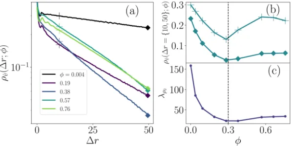
However, as the coverage exceeds φ* in the remaining three subplots, the intermediate-time peak shoulders are suppressed ( Fig. 7b–d ). For this large-distance limit, we characterize ρvˆ( ; )Δr φ by fitting exponential correlation lengths λ φρvˆ( ) (Fig. 8c) to the tails of the curves in Figs. Fitting exponentials to the gnˆ( ; )Δr φ tails to φ the nematic raft peaks, we extrapolate an effective raft size parameter λ φgnˆ( ) (Fig. 7c; inset).
The first is a rest phase, during which each twitcher undergoes no self-induced movement (Figure 1c-1). The third phase is the withdrawal phase, during which the twitcher is actively motile (Fig. 1c-3).
Overview
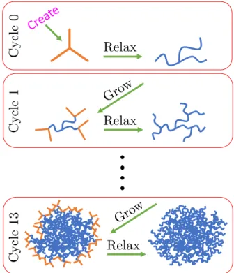
The initial structure of the PGN is built in several cycles, with each cycle containing a growth phase followed by a relaxation phase. In Khatami, Nagel and de Haan [2], the radius of gyration Rg of the PGN is calculated as a function of the simulation time. Thus, the sufficiently stable structure of the PGN during the last 200 ns of the simulation is subsequently investigated with various metrics.
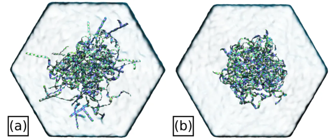
It is natural to wonder what accelerates the relaxation process of PGN from its unphysical initialization to a "hairy colloidal" structure. 4.3(d), indicating that PGN loses polar and unfavorable contacts between water molecules in favor of nonpolar contacts with itself.
Manuscript
This result is somewhat surprising since the inner region of the PGN is indicated in yellow in Fig. Consequently, the water density in this region increases towards the outer shell of the PGN in Fig. This behavior confirms again with both the decrease in the size of the PGN shown in Fig.
Consequently, this section quantifies both the structure and dynamics of the water around the PGN. III C), the dense dendritic structure of the PGN plays an essential role in trapping internal water molecules.
Empirical Results
Equivalence of Indirect and Direct Mobility
Both the indirect and direct simulations are repeated for many choices of the field strength parameterλ and particle sizea. The indirect mobility values calculated from the MFPT of particles initialized from the stationary distribution in the left slit and absorbed in the right slit of the slit well MNFD (as illustrated in Fig.). In addition to the mathematical and empirical demonstrations of the equivalence of µindirect and µdirect, Magill, Nagel and de Haan [3] provide a comparison of the computational costs of the two mobility formulations when both computations are parallelized on a graphics processing unit (GPU).
Runtime plots as a function of the mobility accuracy (shown in Fig. 8 of Magill, Nagel and de Haan [3] attached in App. These results show that the use of the indirect mobility can indeed be a significantly faster alternative to the direct mobility under practical.
Effect of Stationary Distribution
Considering that one of the main motivations behind the use of the indirect mobility formulation is its computational efficiency compared to the direct one. Nevertheless, for the slit-well MNFD currently studied, the steady-state distributions are nearly uniform for almost all choices of the characteristic field strength E∗ and particle sizea (shown in figure). Again the relative errors of the µindirect values with respect to the µdirect values are calculated using Eqn.
The fact that the steady-state distributions of the slit-well MNFD are almost uniform can probably be attributed to the long and narrow slits of the device. This behavior indicates that even when a uniform distribution cannot be used to approximate the stationary distribution, a naive calculation of the stationary distribution is sufficient to obtain accurate indirect mobility values.

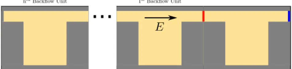
Additional Data - Truncated Backflow
Again, the relative errors of the µindirect values with respect to the true µdirect values are calculated by Eq. The relative errors can be displayed more effectively when plotted as a function of the Péclet number P e=E∗a (Fig. 5.8). When initializing particles in the crevice (bottleneck) of the crevice well MNFD, the indirect mobility calculations appear insensitive to naïve.
Uniform Dirichlet conditions (u=±1) are imposed on the device slots (colored segments in Figure 6.1) to model the voltage drop in the slot domain. A relative error is defined to quantify the accuracy of mobility measurements made with NNM.
Manuscript
Specifically, the NNM is used to solve a model of the electric field in the slit-well microfluidic device, which is an application. 4(c) shows a pronounced relative error in the electric field near the corners at the bottom of the well. Global error statistics for the NNM solutions versus the reference FEM solution, shown against test loss for a variety of network architectures. a) The relative error of the electrical voltages δu[ ˜u].
Summary of the NNM solutions selected for conservation of flux and particle simulation tests. In particular, some of the NNM solutions preserve flux globally approximately as well as the FEM solution.
Manuscript
The domain is intended to represent a single periodic subunit of the slot well device illustrated in FIG. Finally, in the g0 equation [Fig.2(c)], the time dependence of Smoluchowski is implicitly accounted for by integration over all time. Here, g0 has a maximum in the left column near the top of the initial particle distributionρ0.
Throughout Section IV B, four quantities are used to characterize the performance of the NNM over parameter space. Contour plots of the baseline electric potentialal0(black) and fieldE0(red) calculated by the NNM.