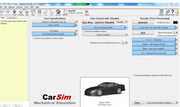
non-linear model predictive control for - bac-lac.gc.ca

Models of simplified 2D vehicle dynamics are developed, discretized and validated against a non-linear CarSim vehicle model. The Gradient Descent Algorithm (Section 3.5) is used to find the optimal solution to the trajectory tracking problem and the optimization of the cost function is subjected to the vehicle dynamics.

Thesis Problem Statement

Organization of the Thesis

Plant Description

Cost Function Description

The cost function 2.5 is called a quadratic cost function because terms of conditions and control are squared. An optimal solution depends on the values of conditions, values of control variable and the shape of the cost function [28].

Constraints Description

In Linear Quadratic Regulator, linear refers to a linear installation and the term quadratic refers to the cost function with quadratic or quadratic factors. The problem that includes both current and terminal costs in the cost function is called a Bolza problem (this type of cost function has been used in this research work).

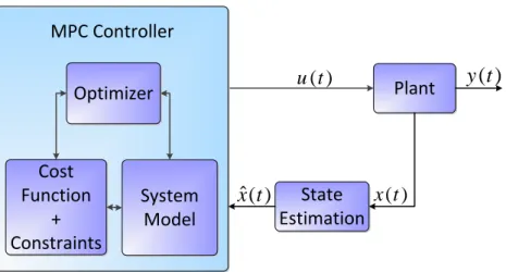
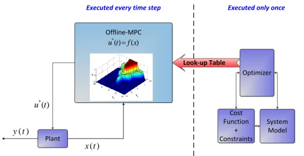
Model Predictive Control

MPC Theory

TheOptimizer finds the optimal control input∗(t) which, when applied to the plant, gives the minimum value of the costJ. It should be noted that these are only the publications named "Model Predictive Control".

Figure 2.2: Model Predictive Controller block diagram

Modern Industrial MPC

Explicit MPC

MPC for Trajectory Tracking

We will now apply the approach as discussed in Subsection VI-A using global Lipschitz continuity of the value function. This chapter focuses on the development of the controller and model formulations used in the rest of this thesis.

Vehicle Modeling

Nonlinear Systems

The state space representation models dynamics of the plant as a set of differential equations in a set of variables. State variable or in short statements is a set of variables that fully describes the system's response to any given set of inputs.

Nonholonomic Systems

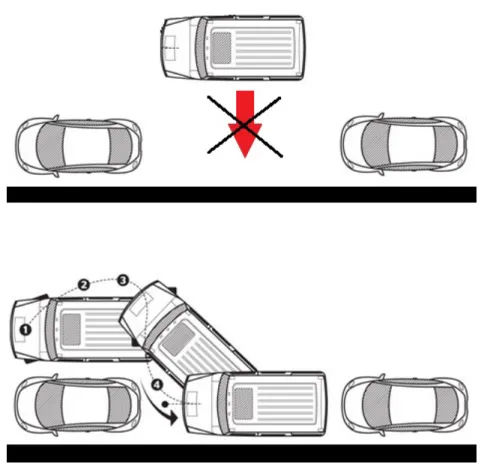
A car must travel in the same direction as its course and cannot travel in any other direction (unless there is a skid). The driver cannot enter the parking space perpendicularly because the van can only roll in the direction of travel (or 180 degrees if reversing).

Mathematical Modeling

The vehicle moves in a two-dimensional plane and (X, Y) are the coordinates of the vehicle in this frame. In this case, the force due to the slope of the road is considered to be zero.

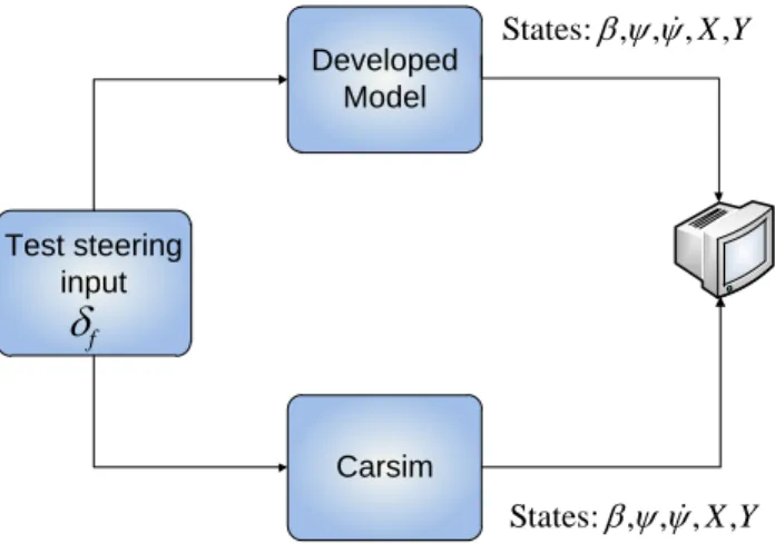
Figure 3.2: Rolling without slipping nonholonomic constraint of a vehicle. Top: Vehicle cannot parallel park directly due to nonholonomic constraint

Model Validation

Validation Setup

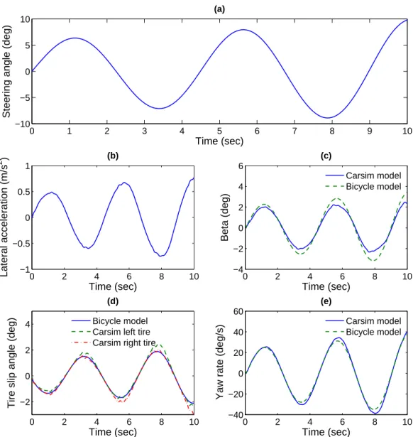
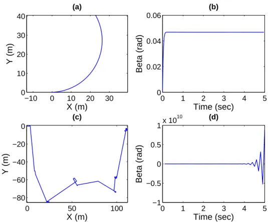
To validate the model, a test similar to Park[72] with an increasing sinusoidal driving signal is performed.

Validation Results

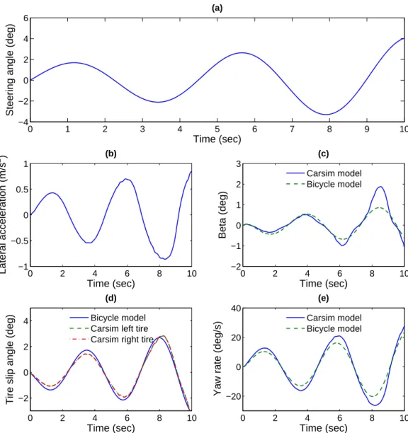
CarSim model left and right tire slip angles differ from each other (Fig. 3.12d), which demonstrates the turning effect in real cars. It can be seen from Figure 3.13d that the CarSim tire slip angles work very close to those of the bicycle model. Third test was performed at a constant speed of 70 km/hand reduced steering angle (Figure 3.14a) input compared to previous test.

The amount of weight transfer depends on the vehicle's mass, speed, steering angle, center of gravity and the distance of center of gravity from the left and right tires (a in Figure 3.17) [91]. More mass leads to more weight transfer, as does a higher center of gravity (h in Figure 3.17). In the first test, a step steering input of 22 degrees magnitude (Figure 3.18a) was applied to the CarSim vehicle moving at 20 km/hand, weight transfer was observed.

Trajectory Tracking using Model Predictive Control

Discretization of Continuous-Time System

Higher order methods are much more accurate than first order methods such as Euler's method (Euler's method is an explicit method). With Euler's method, there is always an associated integration error that is proportional to the sampling intervals. So, in this work, Euler's forward method is used for simplicity of calculations.

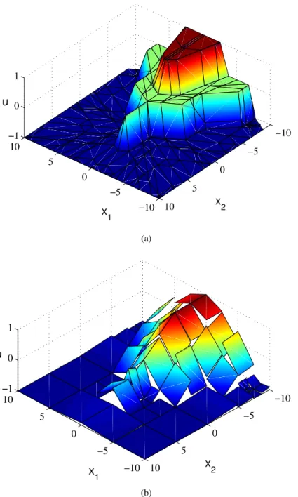
This function is discretized using Euler's forward integration method for discretization intervals and time steps t = k ortk. Figures 3.22a and 3.22b are the output of the model at 33.33 Hz sampling frequency, and the output is very close to the continuous time model frequency. This overshoot is reduced when the model is simulated at 100Hz sampling rate, as seen in Figures 3.22c, 3.22d, and the discrete-time model output closely matches the continuous-time model output.

Figure 3.21a and Figure 3.21b are plots of continuous time model with 0.1 rad steering angle input

Cost Function Formulation

Figures 3.21c and 3.21d show that for the sampling frequency of 1Hz, the trajectory is randomly generated and the system is unstable. The advantage with such a simple function is that it is easily differentiable and does not lead to complex differential terms in the optimization part. For example, the function of equation 3.27 when cut from the basis looks like in figure 3.24.

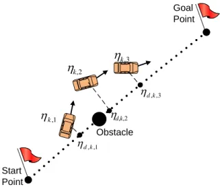
The radius of the circle in this figure can be increased by increasing the weights of the potential function compared to the trajectory tracking weights. Any obstacle shape can be generalized with this simple obstacle method with pointsPk if the nearest point on that obstacle is definable.

Figure 3.22: Stability Anaylsis: (a)Vehicle trajectory at T s = 0.03s, (b) Vehicle side slip angle T s = 0.03s , (c) Vehicle trajectory at T s = 0.01s , (d) Vehicle side slip angle T s = 0.01s

One way is to find the closest point on the reference line using some trigonometric identities and treat this point as the desired trajectory point for the current controller step. One such method has been used by Eklund [56] to repel an aircraft from the nearest boundary point in order to keep it within a fixed predetermined boundary. It may work well to push the vehicle off a boundary, but if used for trajectories following this method may cause the vehicle to pull away once a large obstacle is detected.

When retreating, the vehicle follows the same line, but reverses towards the starting point.

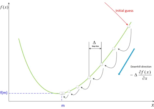
Figure 3.26: Method 1 for trajectory error calculation

Gradient Descent Algorithms

This method is valid only if the gradients can be computed (ie, J is differentiable with respect to each decision variable). Then the slope of the function is calculated ∂f∂x(x) and a step∆ is taken in the negative direction of the slope and the value off(x) is calculated for each point. The process is repeated until the variation inf(x) is zero, and the local minimum of the function is said to be reached at the point x=m.

Equation(3.13) is incorporated into the cost function (Equation(3.12) by introducing a series of Lagrange multiplication vectorsλk(k = 1, .., N). At local minimum of J partial derivative(∂H∂uk .k) ≈ 0which serves as a condition for terminating the optimization loop. Only the first element in the optimized input vector[u∗k]N−1k=0 is applied due to the difference in the identified prediction model and the system to be controlled.

Properties of Gradient Descent Algorithms

Effect of tuning R Setting of the input weighting matrix Has noticeable effect on fine-tuning of the optimization. Constraint Handling A simple method to implement constraints is by projecting the candidate input [u∗k]N−1k=0 onto the constraint set. An accurate but slightly more expensive way of handling constraints is by using the penalty functions.

The advantages and disadvantages of multiple reference trajectory criteria (described in sections) are demonstrated with simulations performed on the fully nonlinear CarSim model. Also, the CarSim mathematical model of the entire vehicle system (aerodynamics, driver, ground) can be extended to Simulink/MATLAB to It is worth noting that CarSim must be active during the simulations, because the S function embedded in Simulink during the runtime uses the CarSim mathematical model and does not contain a mathematical model.

Comparison of Multiple Reference Trajectory Criteria

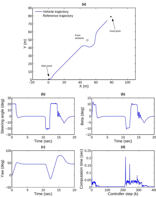
Scenario I: Point Obstacle

In Scenario I, a point obstacle was placed on the planned path of the vehicle and the controller was adjusted according to the parameters in Table 4.1. The vehicle clearly avoided the obstacle by steering away from the obstacle and successfully reached the target point (Figure 4.2). There was a slight difference in the way the vehicle approached the reference trajectory after avoiding the obstacle, but the vehicle heading, side slip and steering angle remained the same in both cases.

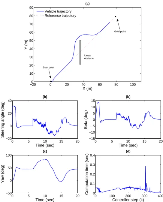
Scenario II: Linear Obstacle

Discussion

Obstacle Avoidance Simulations

Scenario I: Horizontal Road

For this sampling rate and time, the distance of the first horizon at N = 20 and N = 40 was 5.5 mandat11, respectively. From Figure 4.6a it is evident that the vehicle successfully avoided the obstacle by steering to the left and then returned to its right lane. With the longest viewing horizon (N = 40), the vehicle did not immediately turn left, but first turned right.

Such an effect was not seen at the shorter horizon length of N = 20, because when the vehicle detected the object, it did not have enough time to make the expected movement. At horizon length N = 20, the vehicle was found to have moved too close to the boundary from only 1m away from the road edge to avoid the obstacle. At N = 40, the vehicle clearly avoided the obstacle while maintaining a safe distance from the curb.

Figure 4.5: Scenario II: Linear obstacle avoidance using Method 2 trajectory following criterion

Scenario II: Anticipated Move

Controller Robustness Testing

Center of Gravity Variation
Mass Variation
Track Width Variation
Yaw Inertial Variation

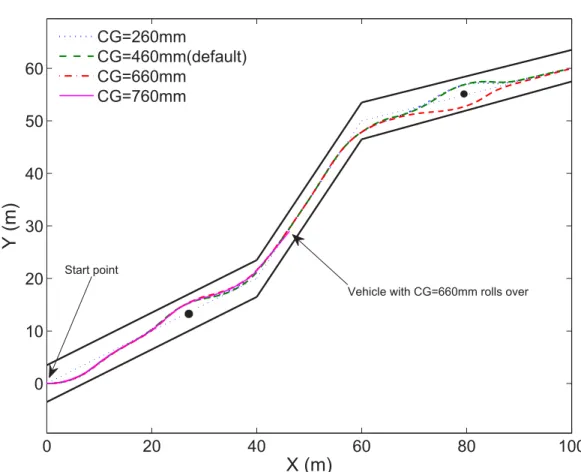
Note the rollover of the vehicle with CG= 760mm so that the cost value is not calculated for this simulation. The vehicle was able to avoid road obstacles and braking with all values of the mass used (as shown in figure 4.14). This is because the tires produce more lateral force which is beneficial for driving the vehicle fast.

For the third test, the vehicle track width (distance between the left and right wheels) was varied and the results are shown in Figure 4.16. The narrow track vehicle (1056 mm) rolled due to high weight transfer during cornering maneuvers. It was observed that the cost of the simulation increased as the yaw inertia increased from the initial value.

Figure 4.11: Vehicle trajectories with different center of gravity (CG) heights. Notice the vehicle roll over with CG = 760mm

Real-Time Analysis

Discussion

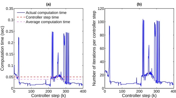
Large computational time steps occur at complex points in the simulation, such as when an object is encountered along the way or when the vehicle steers to approach the reference trajectory. Therefore, if a strict real-time implementation is intended, a counter can be used that breaks the loop if the number of iterations increases25, thus keeping the total processing time within 0.05 s. A mathematical model of the vehicle was derived, and then a nonlinear MPC framework was designed using this model.

The vehicle steering angle was constrained in the cost function formulation, and the obstacle avoidance information was formulated directly within the cost function. The working environment of the vehicle is assumed to be unknown with different types of obstacles. A discretization analysis was performed to find a suitable sampling frequency for a discrete-time plant.

Figure 4.20: Cold start: (a) Computation time for each controller time step, (b) Number of iterations per controller step

Conclusions

Future Work

Available: http://robotics.eecs.berkeley.edu/bear/current research.html [2] “Carsim Product Website,” Mechanical Simulations. Sastry, “Nonlinear model predictive tracking control for rotorcraft-based unmanned aerial vehicles,” in American Control Conference, 2002. Available: http://books.google.com/books?id=PjphGI1 eJYC&dq=Wheel+UK&ie=.

Available: http://www2.control.lth.se/index.php?mact=ReglerPublications,cntnt01, sendfull,0&cntnt01artkey=jsvenPDH&cntnt01year=2007&cntnt01returnid=60 [77, object for avoidance and True Mode of Activities. autonomous ground vehicles," Control Engineering Practice, vol. Bitmead, "Performance and Computational Implementation of Nonlinear Model Predictive Control on a Submarine," in Nonlinear Model Predictive Control, ser.

Discretized equations