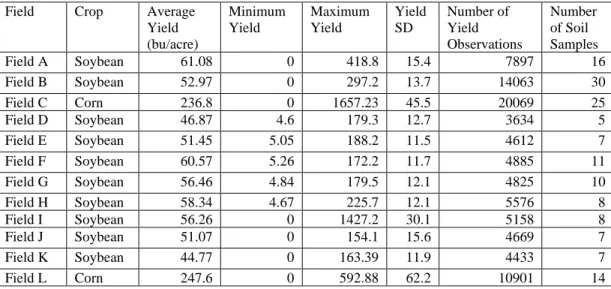
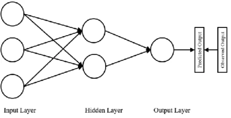
General crop information statistics for 2017 for the seventeen fields used in this study, including crop type for each field. The identity of the fields that had missing yield values for each trial was also included………..…..46. A simplified illustration of the layers and connections of a three-layer artificial neuron propagating back and forth.
Introduction
Moreover, previous research comparing linear and ML techniques often only provides insight into the efficiency of the model's ability to predict yield (Drummond et al., 2003). For example, Drummond et al. 2003) compared artificial neural networks, stepwise multiple linear regression, and design tracking regression. Through this comparison, Drummond et al. 2003) identified artificial neural networks as the most effective method for crop yield.
Literature Review
- Precision Agriculture
- Soil Management
- Topographic Properties
- Crop Yield Predictions
- Machine Learning Models
Knowledge of the spatial variability of soils helps to understand the variability of crop production (Tantalaki et al., 2019). Soil moisture monitoring improves the understanding of water exchange rates at the atmosphere/soil interface (Pasolli et al., 2011). The proportion of humus has a smaller impact on soil fertility, as it is the final product of decomposition (Ketterings et al., 2003).
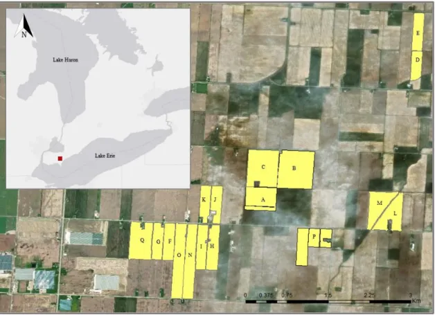
Study Area
Data
Crop Yield and Soil Nutrients Data
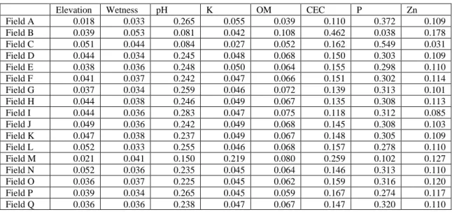
The Olsen method, also referred to as the sodium bicarbonate method, was used to measure the amount of readily available P in alkaline soils. Extractable K was determined using the Mehlich III method in which ammonium ions displace the K cations from the exchange sites. For this extraction, the soil was mixed with a 0.005 M DTPA solution at a ratio of 1 part soil to 2 parts solution and shaken for an hour.
For example, soils with a high CEC will generally have higher levels of clay and OM. CEC was measured as all cations are extracted from an oven-dried soil with ammonium acetate (A&L labs, 2017; OMAFRA, 2009). The number of soil samples taken for each field by grid sampling is also included.
Data Interpolation
Topography Data
The results of the analysis are presented in the appendix and suggested that Kriging, IDW and Thiessen polygons functioned similarly. The yield data were merged with elevation, moisture index, and soil chemistry data to form a single data set.
Methodology
Variograms
In addition, nugget variance may indicate that errors occur during data collection or that samples over a short distance may have significantly different values (Chen et al., 2019). The range is the distance where the variogram reaches the threshold, which represents the largest spatial distance at which the data set can still demonstrate spatial autocorrelation (Chen et al., 2019).
Models and Accuracy Metrics
- Multiple Linear Regression
- Artificial Neural Networks
- Decision Trees
- Random Forest
The fitted model can be used to predict Y values with new additional observed X values (Adamowski et al., 2012). Artificial Neural Network (ANN) can be used to develop empirically based agronomic models (Kaul et al., 2005). Thus, nonlinear relationships that are often overlooked by other techniques can be determined by ANNs with little prior knowledge of the functional relationships (Adamowski et al., 2012; Gopal and Bhargavi, 2019).
A recursive algorithm is used for further assessment of the classification of the attribute with the highest information (Elavarasan et al., 2018). The dataset is gradually organized into small homogeneous subsets while a corresponding tree graph is generated (Liakos et al., 2018). The first node in the tree is called the root node (Gonzalez-Sanchez et al., 2014).
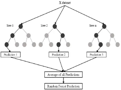
Each internal node in the tree structure represents a different pairwise comparison on a selected feature, whereas each branch represents the result of this comparison (Liakos et al., 2018). A node with outgoing edges is referred to as a test node, whereas a node with no outgoing edges is called a leaf node (Gonzalez-Sanchez et al., 2014). Random Forests (RF) is a non-parametric advanced classification and regression tree (CART) analysis method consisting of multiple decision trees (Jeong et al., 2016).
Additionally, the maximum depth of the tree was set to 30, to aid comparison between the RF and DT models (Gopal and Bhargavi, 2019; Jeong et al., 2016).
Cross-Validation Techniques
Alternatively, the second model of reduction first removed the features with the highest feature importance values. The model reduction technique provided insight into which traits were needed for yield prediction and was used to cross-validate the trait importance analysis.
Results
Spatial Structure Analysis
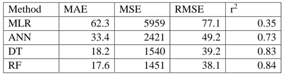
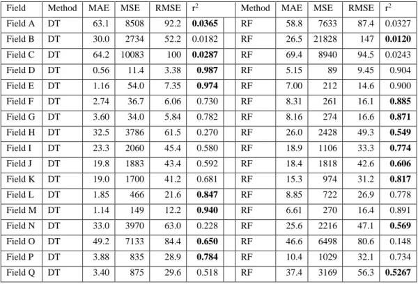
Model Comparison
Features selected at the top of the tree are usually more important than those selected at the end nodes of the trees, as the top splits typically lead to greater information gain (Menze et al., 2009; Sandri and Zucholotto, 2010). The best performing models from the 70/30 training and test analysis, DT and RF, were used in the “Jack-Knifing” cross-validation technique. For the "Jack-Knifing" analysis, one field of yield attributes was deleted and the remaining sixteen field datasets were used to predict the missing yield values.
However, there were three fields identified by the “Jack-Knifing” approach as outliers for both the DT and RF models. P and pH had the highest values in trait importance analysis for fields A, B and C in the "Jack-Knifing" survey. Like the "Jack-Knifing" approach, the "Leave-Group-Out" analysis consisted of deleting the yield data of three fields, while the datasets of the remaining fourteen fields were used for training.
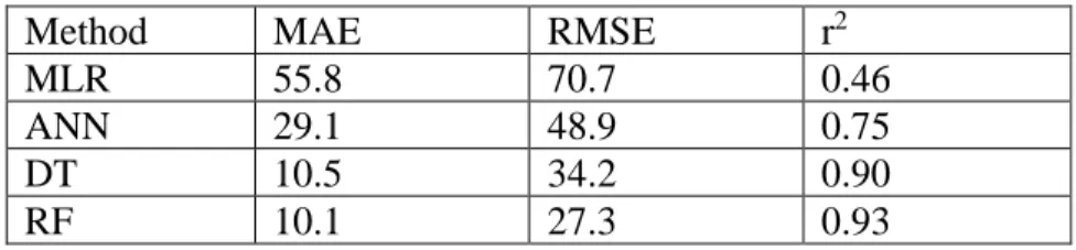
The RF model was selected for this method because it performed slightly better than the DT model in the “Jack-Knifing” study. Trial A consisted of eliminating the yield values for three fields with the highest error in the "Jack-Knifing" analysis. The predicted yields matched the observed data well and the model explained 91% of the yield variation.
The identity of fields that had missing yield values for each trial was also included.
Model Reduction Cross-Validation
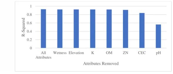
Even with only pH and P traits, which had the highest trait importance values, the model maintained an R-squared of 0.56. The attribute importance values give an indication of which attributes have the highest relevance when predicting yield. The feature reduction method further supports that pH and P are necessary for crop yield predictions for the fields in this study.
Attributes with the lowest feature importance values were then removed one at a time, and the model was rerun after each trial. A second attribute reduction analysis was performed; however, this time, the variables with the highest feature importance values were subtracted first. Although the model still had a high R-squared value and low error metric, this is a significant decrease compared to the first attribute reduction analysis in which the R-squared value decreased by 0.004.
While this is still an acceptable R-squared, the rate at which the R-squared value decreases and the increase in error. When K, altitude, and moisture were the only remaining attributes, the model's R-squared value dropped to 0.73. This helps to support that data quality is more significant than the quantity of data.
Attributes with the highest feature importance values were then removed one by one and the model was rerun after each trial.
Discussion
- Models Comparison
- Yield and Topography
- Yield and Soil properties – All Fields
- Yield and Soil Properties – Individual Fields
- Predicting Missing Data for Multiple Fields
- Sampling Points
RF and DT models have been shown to outperform traditional MLR models in explaining data variability (Breiman, 2001; Jeong et al., 2016). Therefore, it is reasonable that CEC and pH are highly correlated (McKenzie et al., 2004). This process suggests that even if many variables are interrelated and similarly drive the response, only one can influence the RF and DT pattern at the same time (Jeong et al., 2016).
Although there are only two crop types in this dataset, if the models were applied to other areas it would be difficult to account for all the different crops using this technique (Gonzalez-Sanchez et al., 2014). The ranking of the importance of a feature and the partial effect of the variable on the response can be evaluated for systems analysis purposes (Diaz-Uriarte and De Andres, 2006; Jeong et al., 2016; Svetnik et al., 2003; Svetnik et al. ., 2004). Yang et al. 1998), showed by regression analysis that topographic features such as elevation, slope and aspect are significant.
Kravchenko and Bullock (2000), and McConkey et al. 1997) observed higher yields in lower slope positions and lower yields in higher positions. Previous precision agriculture studies with ML are often limited by the limited number of fields and soil sample points (Jung et al., 2006; Drummond et al., 2003). For example, approximately 90% of PA studies registered at the International Precision Agriculture Conference between 1999 and 2004 were conducted in single fields on commercial farms (McBratney et al., 2005).
As described above, Drummond et al. 2003) compared the ML and regression applications and. defined ANNs as the most effective method for predicting crop yield.
Conclusion
This study's result presents the potential for implementation of the RF and DT algorithms to assist in farm management practices. In some cases, this information is able to explain a significant part of yield variability. In contrast, only a small part of yield variability can be explained in other cases.
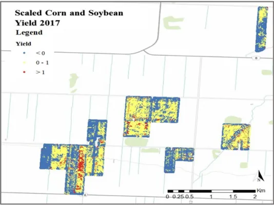
Spatial variability maps showing the distribution of soil and topographic properties of the seventeen fields. Assessment of machine learning approaches for biomass and soil moisture retrieval from remote sensing data. In Proceedings of the first meeting of the scientific advisory committee of the global strategy to improve agricultural and rural statistics, FAO Headquarters, Rome, Italy (Vol. 41).
Machine learning approaches for crop yield prediction and nitrogen status estimation in precision agriculture: A review. Evaluation of the relationship between maize yield spatial and temporal variability and different topographical characteristics. Gonzalez-Sanchez, A., Frausto-Solis, J., & Ojeda-Bustamante, W. Predictive ability of machine learning methods for massive crop yield forecasting.
In Proceedings of the 6th International Conference on Precision Agriculture and Other Precision Resources Management, Minneapolis, MN, USA (pp. 14-17). Data-driven decision making in precision agriculture: The rise of big data in agricultural systems. In Proceedings of the Poster Papers of the European Conference on Machine Learning, Department of Computer Science, University of Waikato, New Zealand.