I would also like to thank Paul for always being there for me and wholeheartedly supporting me every step of the way. We also highlight the contributions of the thesis followed by its organization, summary and impact.
Motivation
Learning these complex intra-connectivity and inter-connectivity patterns in the subgraph and base graph makes this problem challenging. Recent state-of-the-art work (e.g., GLASS [75] and SubGNN [5] ) addresses this shortcoming by the lack of global topology information through the use of labeling tricks [75] or artificially fabricated channels for message passing [5 ].
Contribution
We conduct comprehensive experiments on real-world datasets to show the performance and scalability of our model against various benchmarks, including the current state-of-the-art GLASS [ 75 ]. Through extensive experiments on real-world datasets, we show that SSNP is scalable and outperforms the baselines on 3 out of 4 datasets.
Thesis Organization
Summary and Impact
Experiments show that our variant of POV sampling provides the best performance while being computationally light. In conclusion, our new SSNP with a simple transformation layer together with subgraph neighborhood joining performs well in the subgraph classification task while being scalable (due to node-level operations regardless of the target subgraph). and overcoming the shortcomings of previous works (which require target-specific subgraph operations).
Graph Representation Learning
- Node Classification
- Link Prediction
- Graph Classification
- Subgraph Classification
In the upcoming subsections, we discuss the three prominent downstream tasks in graph representation learning: node classification, link prediction, and graph classification, and different graph neural network architectures targeting specific tasks or all tasks in general. Other SGRL methods such as SEAL [94] and DE-GNN [48] use enclosing subgraphs together with labeling tricks for link prediction.
Shallow Encoders
Thus, subgraphs can be considered an abstract data type for nodes, links, and graphs, and subgraph classification can be considered a more general problem. Existing works on node classification, link prediction, and graph classification cannot be directly extended to subgraph classification, since subgraphs have both internal and external topology.
Message Passing Graph Neural Networks
Graph Convolutional Networks
Node representations are obtained by summarizing over the messages from the neighboring nodes and the node itself. However, GCN can be used in transductive settings for various downstream tasks such as node classification and link prediction.
GraphSAGE
Subgraph Classification by MPGNN
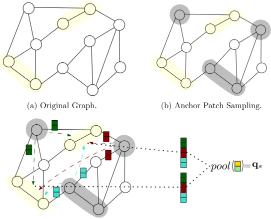
SubGNN
For internal position and boundary position, a node from the subgraph and a group of nodes from the base graph are used as anchor patches. For internal and boundary neighborhoods, nodes from the subgraph and nodes from the h-hop subgraph neighborhood are used as anchor patches. A is then used to propagate messages to each component of the subgraph as shown in Equation 2.6.
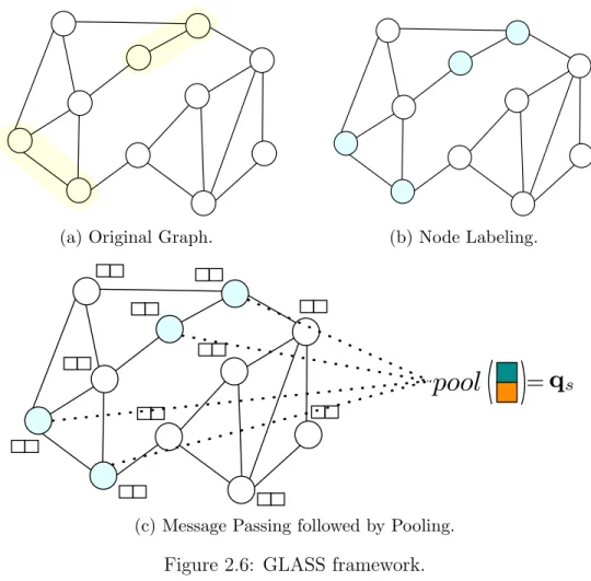
GLASS
The maximum zero-one labeling captures the maximum number of distinct labels generated for each node by all subgraphs in the mini-bundle. However, the maximum number of zero-ones is as efficient as marking zero-ones if the two subgraphs in the miniseries are far apart. While the at-most-zero-one labeling trick eliminates the need for subgraph extractions, the labeling depends on the number of subgraphs in each miniseries, and the graph must be relabeled whenever a miniseries is created.
Data Augmentation in Graphs
Moreover, such an approach using two separate features and blending works better to prevent smoothing of labels in the graph.
Graph Contrastive Learning
DeepWalk uses random walks to understand the neighborhood around each node and encodes the sequence of random walks as a representation of the nodes. An extension of Deepwalk, node2vec [29] introduced two hyperparameters to control the trade-off between breadth-first and depth-first exploration for random walks. In addition, hyperparameters such as the number of random walks and the random walk length used to create random walk-induced subgraph neighborhoods can be considered similar to the node2vec parameters, p and q that provide a trade-off between local and global structure. .
Message Passing Graph Neural Networks
This allows the node representations to be similar to nodes belonging to the same group and thereby get better representations. Our model can use any of the MPGNNs as a transformation layer to generate the node embeddings used for generating the subgraph and its neighborhood embeddings. By using SSNP, the expressive power of the subgraph representations created by the underlying MPGNN can be improved.
Subgraph Representation Learning
For example, shaDow-GNN [92] extracts K-hop subgraphs around each node and operates on them for node classification. Similarly, NGNN [96] aggregates the node features of the K-hop rooted subgraphs around each node to increase the expressiveness of representations for graph classification. Relation to this thesis SSNP is based on the idea that wrapping subgraphs around a few nodes can provide more information and result in better representations.
Subgraph Classification
Using the original subgraph and multiple extended views, it is possible to create different subgraph representation vectors for the same original subgraph. Each view, including the original subgraph, is then passed to a specific subgraph model to obtain its embeddings. The individual embeddings of each subgraph view are then combined to give one final subgraph embedding.
Scalability of SGRLs
By setting the hyperparameters of the random walk to an appropriate value, it allows comparable performance with significant computational gains. Furthermore, SUREL does not use subgraphs induced by a random walk, but only random walk sequences. In addition, the relative positions of nodes appearing in random walks are recorded by vectors called relative position encoding (RPE).
Scalability by Sampling
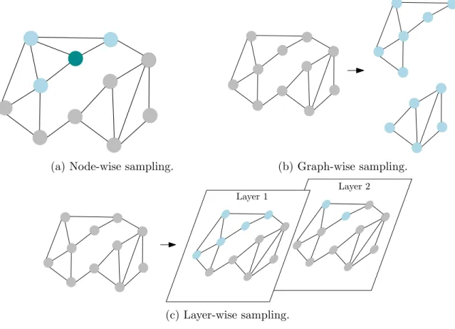
FastGCN [14] is an extension of the traditional graph convolution network that performs layer-wise sampling of the vertices in the graph to enable inductive learning and reduce computational complexity. While GraphSAGE performs neighbor sampling at each layer, FastGCN performs layer-independent sampling of the nodes themselves, which significantly reduces the overall complexity of the model. In addition, SSNP can work with graph neural networks that use any of the above sampling techniques for further scalability.
Problem Statement
Transformation Layer
In addition to introducing MLP as a transformation function, we considered two convolution layers of the graph. Our nested network (NN) convolution follows the network-within-a-network architecture [69] as a way of deepening the GNN model by adding more nonlinear layers within the convolutional layer to increase the performance of the model while avoiding overfitting and smoothing.
Subgraph Neighborhood Pooling and Variants
Compared to the exact subgraph neighborhood which can become extremely large, the size of sparse subgraph neighborhoods is bounded by hk, which is the product of i. Our neighborhood of h-hop-reduced subgraphs has a similarity to surrounding subgraphs of random samples [50], but differs in two ways: the neighborhood does not include the original subgraph, and the neighborhood is defined over subgraphs of arbitrary size (instead of pairs of nodes ). Given the computational and learning advantages of specified neighborhood subgraphs, we introduce stochastic subgraph neighborhood joining (SSNP) with a slight modification of Eq.
Expressiveness of Subgraph Neighborhood Pooling
Subgraph Neighborhood Sampling Strategies
However, the dataset size and training time grow linearly with the number of views n.v. In the preprocessing stage similar to PV, POVnvcreates multiple split subgraph neighborhoods (i.e., multiple views) for each subgraph. POV allows data augmentation with multiple views, while keeping the number of training instances per epoch independent of the number of views nv.
Evaluation Metric
-label No No Yes No Table 5.1: Statistics of all real-world datasets. the metabolic disease that corresponds to a group of phenotypes. The classification task in hpo-neuro is to predict the neurological disease corresponding to a group of phenotypes. In em-user we want to predict the gender of the user given the exercise history subgraph.
Baselines
Experimental Setup
We always set the number of walks per node = 1, and let the pooling method for the subgraph and the neighborhood be the same (i.e. pools = pooln). Unless otherwise noted, we use the POV to create subgraph neighborhood views, setting the number of views nv = 20 and the number of views per epoch nve = 5. Our model is implemented in PyTorch Geometric [24] and PyTorch [59].2 Our results are reported with an average F1 score over 10 runs with different random seeds.
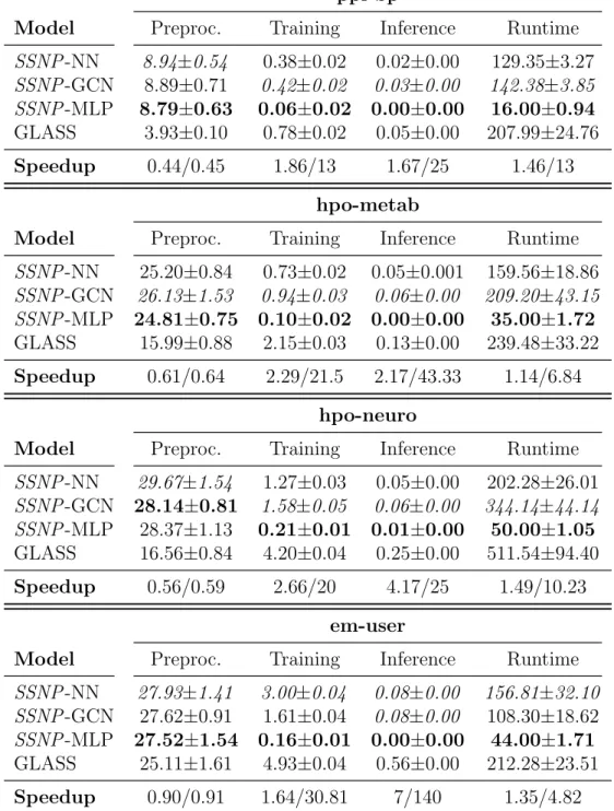
Results: F1 Score and Runtime
SSNP-NN performs better than other baselines in hpo-neuro which has dense subgraphs similar to hpo-metab, the task in hpo-neuro (i.e., multi-label classification) is fundamentally different from the task in hpo-metab (ie, multiclass classification). Moreover, hpo-neuro contains about twice as many subgraphs as hpo-metab, which may attribute to the better performance of our model in hpo-neuro. SSNP-MLP also appears to be relatively competitive ranking third in hpo-neuro and em-user.
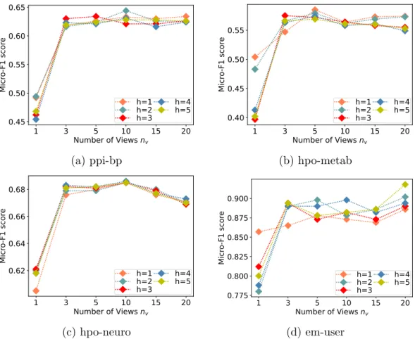
Multi-view Hyperparameter Analyses
In em user, setting h to 3 and nve to 10 gives the best performance, but incurs additional training overhead (see Figure 5.6b). We believe that this performance is primarily due to access to large enough extended training data and the regularization offered through the stochasticity of sampled views per epoch. In summary, SSNP with small random walk length and number of views per epoch provide comparable or better results while maintaining a light computational load and allowing for faster training and inference.
Results: Stochastic Pooling Strategies
Summary
A simple POV data augmentation technique allows model generalization without additional computational cost. Our model, combined with our data augmentation techniques, outperforms current state-of-the-art subgraph classification models on 3 out of 4 datasets with a speedup of 1.5-3×. Our model, with simple transformation layers such as MLP, overcomes most of the subgraph classification baselines during re-transformation.
Future Directions
Reusing Random Walks
Efficient Subgraph Neighborhood Selection
Graph Contrastive Learning
In Proceedings of the 25th ACM SIGKDD international conference on knowledge discovery and data mining (2019), pp. In Proceedings of the Sixteenth ACM International Conference on Web Search and Data Mining (2023), pp. In Proceedings of the 24th ACM SIGKDD International Conference on Knowledge Discovery & Data Mining (2018), p.
Node Classification Example
Link Prediction Example
Graph Classification Example
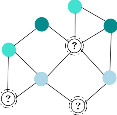
Subgraph Classification Example
SubGNN architecture
GLASS framework
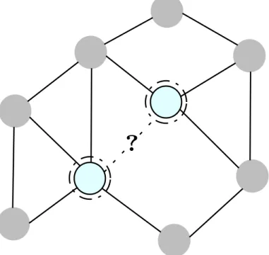
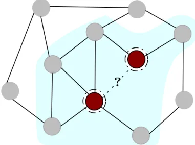
An example of SGRL framework SEAL
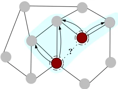
An example of scalable SGRL framework ScaLed
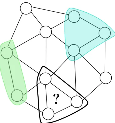
Different sampling techniques
Architecture of our model
The randomness in the neighborhood subgraph also adds some regularization effect to the training of the model (similar to what was observed in ScaLed [50]). In Proceedings of the 16th International Conference on Extending Database Technology (New York, NY, USA, 2013), EDBT ’13, Association for Computing Machinery, p. In Proceedings of the Sixteenth ACM International Conference on Web Search and Data Mining (2023), pp.
In Proceedings of the IEEE/CVF Conference on Computer Vision and Pattern Recognition (2020), p. In Proceedings of the 20th ACM SIGKDD International Conference on Knowledge Discovery and Data Mining (2014), p.
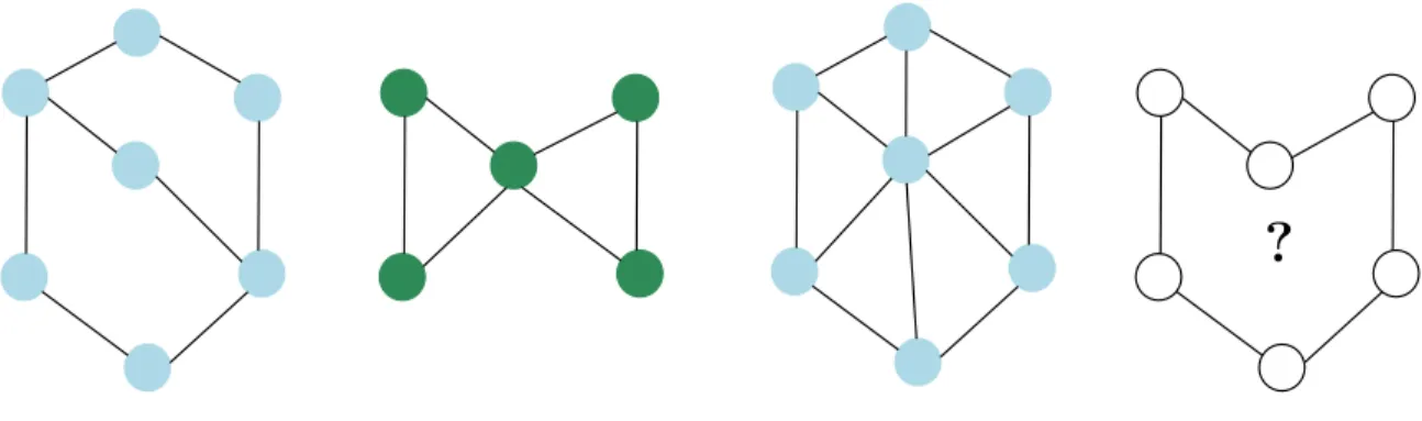
Comparison of subgraph pooling vs subgraph neighborhood pooling
POV Sampling Strategy
Confusion Matrix
Effect of number of views in PV
Effect of number of views per epoch on ppi-bp
Effect of number of views per epoch on hpo-metab
Effect of number of views per epoch on hpo-neuro
Effect of number of views per epoch on em-user
Effect of sampling strategies on pre-processing time and training time