A thesis submitted in conformity with the requirements for the degree of Doctor of Philosophy

The effectiveness of the unsteady optimization algorithm is demonstrated by applying it to several problems of interest, including shock tubes, impulses in converging-diverging nozzles, rotating cylinders, transonic shock, and an unsteady trailing edge flow. 108 5.55 Drag coefficients for the original 30P30N lamella position and a perturbed position.109 5.56 The sensitivity of the gradient components to the step size of the finite-.

L IST OF S YMBOLS

NB number of grid blocks Nc number of coarse time steps Ncon number of constraint equations N(dB) overall sound pressure level NF number of flow variables O objective function. O∆E Ordinary Differential Equations OASPL Overall Sound Pressure Level ODE Ordinary Differential Equations PDE Partial Differential Equations Sequential Quadratic Programming SQP.

I NTRODUCTION

Aerodynamic Design using Numerical Optimization

Gradient-based methods are probably the most effective for aerodynamic design problems, as significant design improvements can be achieved with relatively few objective function evaluations. The main challenge for the implementation of gradient methods is the accurate and efficient calculation of the gradient.

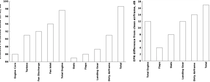
Introduction to Aircraft Noise

Thus, eliminating one of the sources would only result in an insignificant noise reduction of 3dB. The noise comes mainly from the flow near the side edges of the flap, associated with flow separation in the crossflow of the flap [17].

Figure 1.1: Common environmental sound levels [135].

Objectives and Outline

Develop an efficient unsteady aerodynamic optimization algorithm based on a Newton-Krylov and coupled approach, where the underlying physical model is the unsteady Reynolds-Averaged Navier-Stokes (URANS) equations. The development and application of this unsteady aerodynamic optimization algorithm and hybrid acoustic prediction optimization algorithm is also presented in Rumpfkeil and Zingg.

G OVERNING F LOW E QUATIONS

Navier-Stokes Equations

Turbulence Model
Thin-Layer Approximation and Coordinate Transformation

Spatial Discretization

Boundary Conditions

Temporal Discretization
Solving the Nonlinear System

The Linear Problem

The spatial discretization scheme of the thin-layer Navier-Stokes equations (2.20) is that used in ARC2D [112] for C- or O-topology meshes and TORNADO [96] for H-topology meshes. The spatial and temporal discretization of the thin-layer Navier-Stokes equations (2.20) leads to the nonlinear systems O∆E (2.45) and (2.47), respectively.

Table 2.1: Butcher table for a six-stage ESDIRK scheme.

U NSTEADY O PTIMIZATION

Formulation of the Discrete Time-dependent Opti- mal Control Problem
Design Variables and Grid-Perturbation Strategies
The Discrete Adjoint Approach for the Gradient CalculationCalculation
Optimizer

Finally, one can evaluate the gradient of the objective function J with respect to the design variables Y, as follows. Thus, the gradient of J is fully determined by the solution of the coupled equations in reverse time from the final flow solution and the partial derivatives of the objective function, constraints and residuals with respect to the design variables (while ˆQn is kept constant).

N OISE P REDICTION T ECHNIQUE

Acoustic Wave Propagation Modelling

The Kirchhoff approximation is based on an inhomogeneous wave equation derived by assuming that the required acoustic pressure fluctuation (p0 = p−p∞) and its time and normal derivatives are examined on a near-field surface located within the linear flow located. region. In contrast, the FW-H approach [41] is an exact rearrangement of the continuity and momentum equations. The time history of all flow variables on the near field surface is required, but their temporal or spatial derivatives are not needed.

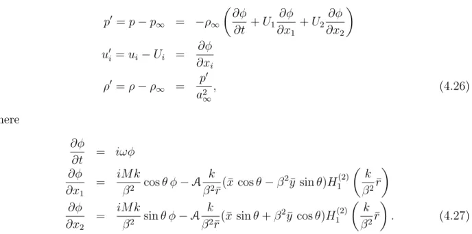
The 2D FW-H Equation in the Frequency-Domain

Thus, Lockard [77] assumes a uniform rectilinear motion of the control surfacef =f(xi+Uit), where Ui is a constant velocity of the surface. Its derivation, outlined below, proceeds by using the Galilean transformation of Eq. 4.6) The surface velocity has been replaced by −Ui, which can be deduced from f(xi+Uit) = 0. The Green's function G of this convection Helmholtz equation for M < 1 is obtained from the Prandtl-Glauert transform of the 2D Green's function in free space in the frequency domain.

Figure 4.2: The window function used to make the input data periodic.

Validation

Monopole in Uniform Flow
Scattering by an Edge
Airfoil in Laminar Flow

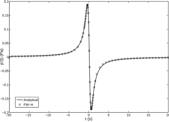
The pressure fluctuations over time shown in Figure 4.7 exemplify the behavior of the source terms for large negative and positive times. The directivity comparison between the exact and calculated solutions for observers at a radius of 50m from the edge is shown in Figure 4.6, and the time histories of the pressure fluctuations at r = 50m and −45◦ from the bottom surface of the half-plane are compared in Figure 4.7. The agreement at the first probe location is also quite good, except for the underprediction of the amplitude by the FW-H calculation.

Figure 4.3 compares the directivity from the FW-H calculation to the analytic solution in the far-field at r = 500 m, and Figure 4.4 makes a comparison for the time histories of the pressure fluctuations at x 1 = 500 m and x 2 = 0 m

R ESULTS

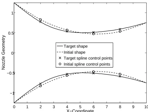
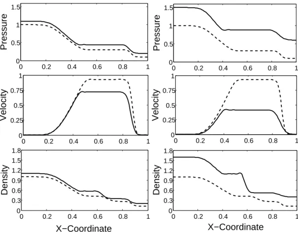
Pulse in 1D and 2D Converging-Diverging Nozzle

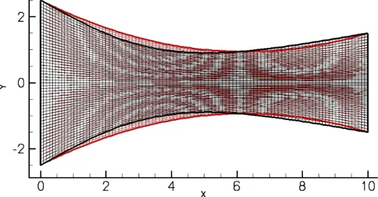
The initial and target shapes of the nozzle, along with the locations of the control points, are shown in Figure 5.1. To measure the accuracy of the adjoint gradient (ad), it is compared to the gradient calculated via the complex step method (cs) [133] in the first design iteration. The x-locations of the control points are 2.5, 5.0, and 7.5, respectively; the initial and target shapes of the nozzle are shown in Figure 5.4, where the grid consists of 99×55 nodes.

Figure 5.1: Initial and target converging-diverging nozzle shapes.

The Inverse Design of Flow in a Shock-tube

Again, the obtained adjoint gradients of the cost functionals with respect to the design variables in the first design iteration were compared with those calculated by the complex steps method [133].

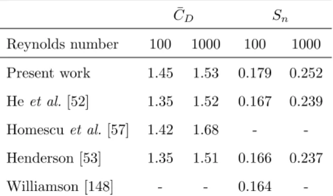
Figure 5.7: Pressure, velocity and density: initial guess (dashed line) and target observation (solid line) at t = T = 0.21 using Y 1 ∗ in the left column and Y 2 ∗ in the right column.

Drag Minimization for Viscous Flow around a Ro- tating Cylindertating Cylinder

It is very important to have a practical knowledge of the design space to be able to choose a reasonable time step and control window. The rotation starts impulsively, and after a transition period of about 1500 steps, the average drag coefficients of the rotating cylinders are all smaller than the average drag coefficient of the stationary cylinder. This optimum value minimizes the average drag value well outside the range of the control window, as can be seen in Figure 5.9; this behavior has also been observed by other researchers [57, 52].

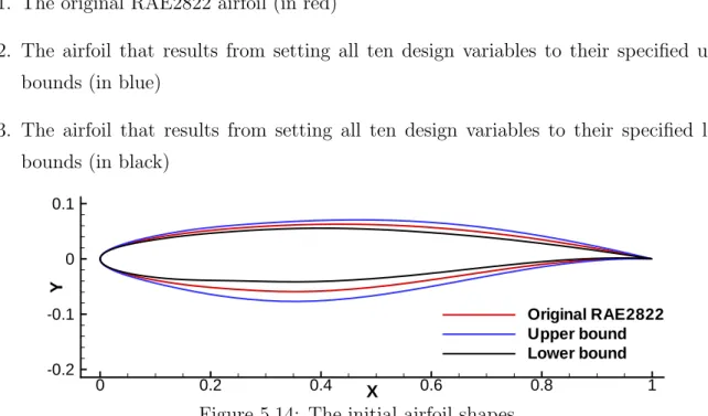
Table 5.1: Mean drag coefficients and Strouhal numbers (the last two are experimental results).

Transonic Buffeting Shape Optimization

For mean drag above mean lift minimization, all three initial shapes converge to the same final shape shown in green. However, for average drag minimization, each initial shape leads to a slightly different improved shape. Starting from the original RAE2822 airfoil, it leads to the best shape with about 17 percent reduction in average drag.

Figure 5.14: The initial airfoil shapes.

Aeroacoustic Shape Design for Unsteady Trailing- Edge FlowEdge Flow

The objective functions are always scaled to the initial value of the original Blake airfoil objective function (J) to make comparisons easier. A comparison of the average lift and drag coefficients for the original and improved airfoils is shown in Table 5.6. The time histories of CL and CD for the original Blake airfoil and the best airfoil after optimization are shown in Figure 5.27.

Figure 5.20: Instantaneous pressure coefficient contours of the initial Blake airfoil.

Remote Inverse Designs

A Single-element Airfoil in Unsteady Turbulent 2D Flow
A Multi-element Airfoil in Unsteady Laminar 2D Flow

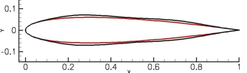
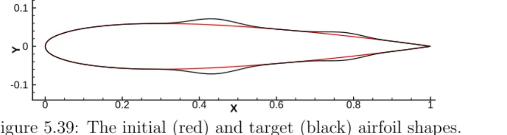
Furthermore, in Section 5.6.2 the remote inverse design of the NLR 7301 multi-element configuration [144] at a high angle of attack in unsteady laminar flow is addressed. The initial airfoil shape is NACA 0012 and the four shape design variables are slightly perturbed to obtain a target airfoil shape, as shown in Figure 5.28. The choice for the near-field plane in this case is shown in Figure 5.29, and the required pressures are simply taken at the network nodes.

Figure 5.28: The initial (red) and target (black) airfoil shapes.

Remote Inverse Design Using Hybrid URANS/FW-H

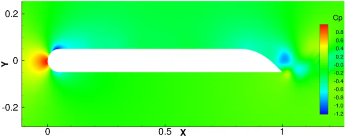
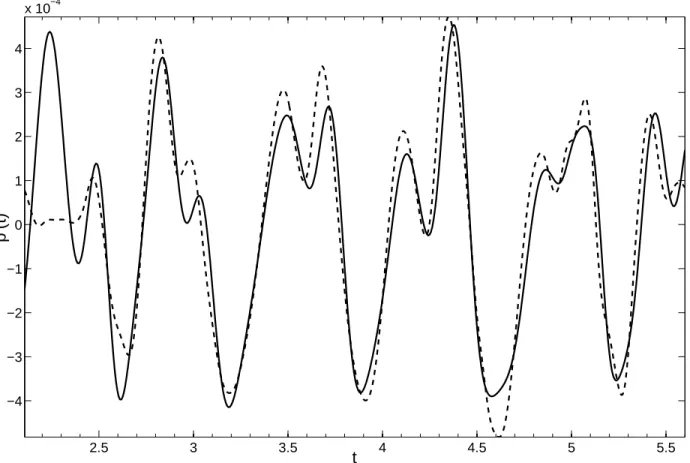
If we try the same approach for the second case, namely storing the flow field only every fourth and tenth time step, it produces a different result (see Figure 5.37). Nevertheless, the comparisons of pressure fluctuations calculated by CFD and FW-H for the initial NACA 0012, as shown in Figure 5.40, show good agreement for both time march methods at a point approximately two chord lengths below the trailing edge. The convergence history of some remote inverse form design problems using the hybrid URANS/FW-H optimization algorithm is shown in Figure 5.42.

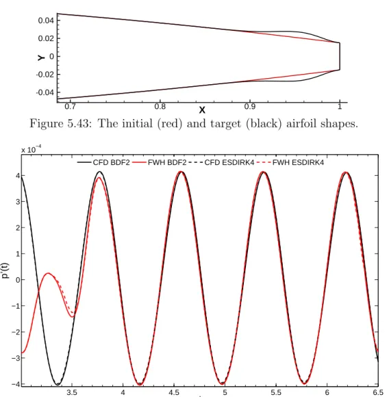
Figure 5.39: The initial (red) and target (black) airfoil shapes.

Turbulent Blunt Trailing Edge Flow

The convergence history of the remote inverse shape design problem for a turbulent trailing edge flow using the URANS/FW-H hybrid optimization algorithm is shown in Figure 5.46. Results for such small values of the objective function in combination with the more complicated time marching method. The objective function values are always scaled to the average drag value of the original airfoil, JD to make comparisons easier.

Figure 5.43: The initial (red) and target (black) airfoil shapes.

High-lift Noise Optimization

Second, the velocities in the recirculation zone of the slat zone are relatively small leading to correspondingly small Reynolds numbers. Only two design variables are used in the optimization, namely the horizontal and vertical translations which control the position of the slat. However, the optimizer managed to reduce the objective function value in one of the runs by almost forty percent given the slat position.

Figure 5.53: Comparison of pressure fluctuations calculated by CFD (solid) and FW-H (dashed) about 1 4 c below the slat trailing edge.

C ONTRIBUTIONS , C ONCLUSIONS

AND R ECOMMENDATIONS

Some of the investigated problems yielded novel and counterintuitive results, such as wavy airfoils in Section 5.5 and the bulge near the open trailing edge in Section 5.8. However, very noisy design spaces were also encountered (e.g. rotating cylinder, trailing edge laminar flow, and above all the high-lift noise reduction problem) where the gradient rates were hardly reduced, even though the value of the objective function was significantly improved. An improved initial guess for solving coupled linear systems can greatly reduce the computational effort.

R EFERENCES

48], Application of Ffowcs Williams/Hawkings equation to two-dimensional problems, Journal of Fluid Mechanics, Vol. Howe, A Review of the Theory of Trailing Edge Noise, Journal of Sound and Vibration, Vol. Lockard, An efficient two-dimensional implementation of Ffowcs Williams and Hawking's equation, Journal of Sound and Vibration, Vol.

A PPENDICES

Appendix A

T HE D ISCRETE AND C ONTINUOUS

A DJOINT A PPROACHES

The exact gradient of the discrete objective function is obtained, which means that the optimization process can fully converge. On the other hand, the advantages of the continuous approach are: a) The physical meaning of the adjacent variables and the role of the adjacent boundary conditions are much clearer. This better understanding of the nature of the complementary solutions is especially beneficial when approaching more difficult problems, e.g.

Appendix B

A DJOINT E QUATIONS FOR BDF2

Appendix C

D ERIVATION OF THE FW-H E QUATION

Finally, the dipole term Fi and the monopole term Q are defined as follows Fi = [ρui(uj −vj) +pδij −τij]∂f.

Appendix D

WITH T IME S TEP S IZE C HANGE

Adjunct Equations for BDF2 with Change in Time Step Size The problem of minimizing a discrete objective function J as given by Eq. 3.3) is then equivalent to the unconstrained optimization problem of minimizing the Lagrangian function. Some caution must be taken when calculating derivatives of RNc+1 with respect to ˆQn, as the factors before ˆQNc+1, ˆQNcan and ˆQNc−1 deviate slightly from the usual scheme.

Appendix E

A DJOINT E QUATIONS FOR

ESDIRK4 WITH T IME S TEP S IZE C HANGE

Associated equations for ESDIRK4 with time step size change with respect to ˆQnk and ψnk for n= 1,.

Appendix F

I MPLEMENTATION D ETAILS OF THE

FW-H E QUATION

Note that variables with index J+ 1 have the same value as those with index 1. Differentiation with respect to the flow variables. If the FW-H equation is used as part of an objective function in the optimization framework, the derivative of the far-field pressure fluctuations with respect to the flow variables is explicitly needed. Denotes the nondimensional conservative variables given by Eq. 2.1) at the source node j and time step n as Qnj, the derivative of the far-field pressure fluctuations in the frequency domain with respect to the flow variables is given by:.