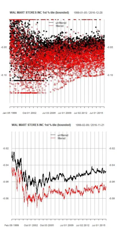
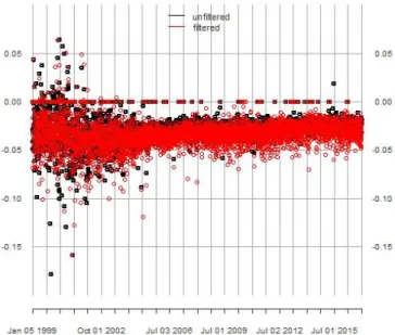
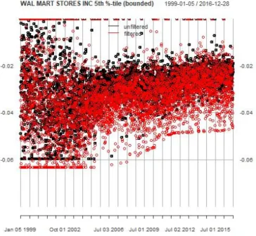
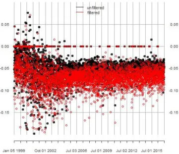
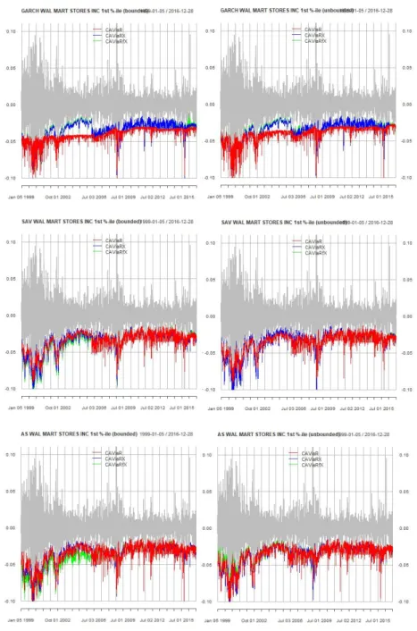
11 3.1 Walmart sentiment score (unfiltered versus filtered) at 1% quantile. point observation and 20-day rolling average) without score truncation/cleaning (unlimited). 26 3.2 Walmart sentiment score (unfiltered vs. filtered) at 1% quantile. point observation and 20-day rolling average) with score truncation/cleaning (bounded). 28 3.4 Walmart sentiment score (unfiltered vs. filtered) at 5% quantile. point observation and 20-day rolling average) with score truncation/cleaning (bounded).
Introduction
In the field of natural language processing, sentiment analysis assesses the implicit sentiment associated with specific words, sentences, and general text or spoken words. A section of text can be interpreted as a series of sentences that are themselves a series of words. Such a process may include associating words as positive or negative and assessing the combined effects of those words in determining sentiment for sentences and larger bodies of text; see Tetlock et al.
Sentiment and Measurement
One of the earliest and most widely used methods is the creation of lexicons or specific lists of words. A stock's abnormal return is the difference between individual stock returns relative to the value-weighted CRSP index over three days. Dk,t is the number of articles written about company k in time t. F Qd,j,k,t is the number of times word j occurs in clause d. Nd,k,t is the number of words in clause d.
Sentiment and Risk Management
In the parametric approach, the estimated standard deviation of the return distribution of a volatility model is translated into the VaR quantile. The use of CAVIaR models in addition to sentiment analysis is new and there is no known previous research into their application. We aim to replicate this approach, but use a textual sentiment score as the regressor instead of the implicit quantile.
Value-at-Risk and Backtesting
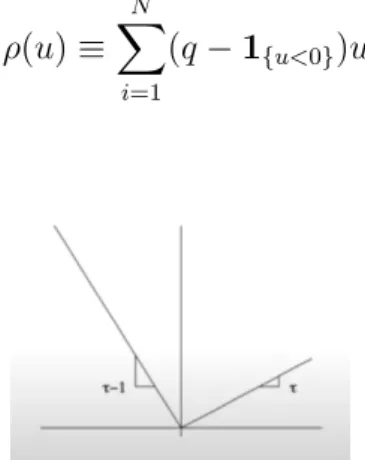
To calibrate the CAViaR model, the parameter vector, ˆβ, is the argument that minimizes the quantile loss function in equation 1.14. Essentially, a VaR model that predicts the q-th quantile of returns should neither overestimate nor underestimate the quantile level of risk. The DQ test uses a linear regression model to test the independence of the hit indicator, Hitt(q).
Therefore, testing for joint nullity of the coefficients would check for correct conditional coverage. The quantile loss is the same as that used by Koenker & Bassett Jr (1978) for quantile regression. The quantile loss is an asymmetric loss function that penalizes more by weight (1 -q) observations of exceeding VaR.
Given two hit indicator sets, A and B, the quantile loss ratio is the ratio of the average quantile losses for both A and B. The closer the absolute value of the AE ratio is to 1, the better the model. An AE ratio < 1 is considered too conservative, with the model making fewer hits than expected, and an AE ratio > 1 is considered to underestimate the risk, with the model making more hits than expected.
Overall, we aim to look for improvements between the baseline models and the models that are augmented with our generated sentiment score for the three VaR backtest metrics.
Fama and French Factors
Out of 598 companies, only 100 companies are selected for VaR analysis based on those with the most average forward frequency observations (equation 1.6).
Average Term Frequency
Regression 1: Linear Regression
The series of returns of companyi(i k}) are regressed to the corresponding Fama-French factors using linear regression. Ri is a Ti×1 vector of daily stock returns for companyi with a time frame of length Ti. F Fi is a Ti×5 matrix of the corresponding five Fama-French factors over the time frame of company i.
Therefore, the purpose of βi is to consider the coefficient of company i to systematic market factors. The goal of the second regression is to assess whether additional predictive power emerges from average word frequency.
Regression 2: Quantile Regression
F reqi,t−1 is a Ti×V matrix of one-day lagged (t-1) mean term frequencies (1.6) for a lexicon vocabulary of V words over time frameTi for company i. Λq is a V ×1 vector of vocabulary coefficients, λv,q, to the mean term frequencies for the specified quantile, q. This one-day lagged quantile regression aims to test whether the mean term frequencies have predictive power for a given quantile of residuals and indirectly the returns.
SCOREq,i,t is estimated by quantile regression using a sparse implementation of the Frisch-Newton interior score algorithm described in Portnoy &. With the exception of the first year of data, the sentiment coefficients for a given year were calibrated using data up to one year earlier. For example, a sentiment score compiled in 2009 would use data from 1999-2008 as a window to obtain estimated sentiment coefficients.
Sentiment scores were constructed from the first available frequency observation for each company to its last frequency observation. The number of frequency observations per company varies over the time frame, and if no news is observed for a company at time, the average term frequency, f(v, i, t−1), and hence the sentiment score, SCOREq, i,t , would be 0 at that point.
Lexicon Selection
Perform the first regression using linear regression (Equation 3.1) on the returns using the Fama-French factors as independent variables and obtain the residuals, ηi,t for all firms. For a given quantile, q, perform two quantile regressions on Equation 3.2 to estimate the q quantile and the (1−q) quantile of the residuals, respectively. Remove words that have the opposite sign from both sets of quantile regression coefficients, Λq,unfiltered and Λ1−q,unfiltered, to obtain a new set of words, Vf-filtered.
Perform step 1 again and use quantile regression with equation 3.2 on the obtained Vf filtered to the desired quantity q to obtain a final set of coefficients, filtered Λq,f, for the dictionary, filtered Vf. Thus, two sets of sentiment scores were constructed with vocabularies and coefficients, {Vunf iltered,Λq,unf iltered} and {Vf iltered,Λq,f iltered}. Average thermal frequencies can sometimes exhibit extreme behavior due to the unpredictable behavior of the news/media cycle.
Since the residuals,ηi,t, are indirect components of the company's return, the residuals should normally lower the mean return in equation 3.1, when the lower return quantiles are taken into account (i.e. then, when the CAViaR model is used for the month of January 2006), the sentiment observations are truncated by 0 and the empirical 5% quantile observed in the calibration window as cutoffs Thus, for each company we have two sets, each with two series of sentiment scores.
The top half per figure is the point observations and the bottom half of the figure is the 20 day moving average to distinguish the trend.
CAViaR model calibration
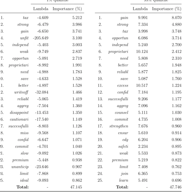
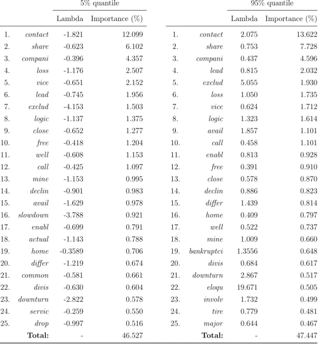
The frequency coefficients were collected and the importance (A.1) of vocabulary words was observed. The cumulative importance of the top 25 words is relatively high (over 40%), meaning that they account for a large degree of variability within the score. For example, Table 4.1, which shows the importance of words after the first quantile regression before filtering (1% vs. 99% quantile), the root words contact, share, exclude and compani are among the top 5 for both regressions. at the 1% quantile and at the 99% quantile.
In Table 4.1, words such as unfit (4th), deficit (6th), decline (15th), junk (16th) and delay (25th) are among the top 25 words for the first quantile and are not present in the top 25 words for the corresponding high quantile regression at the 99th quantile. However, we see that in Table 4.3, first quantile regression before filtering (5th vs. 95th quantile), these words both become present in the top 25 words. In Table 4.2, unsuitable (4e) is present in both the first regression and the second subsequent filtration.
In Table 4.2, other words, including 'disappoint' (15th) and 'warningari' (16th), are also among the top 25 words for the low quantile (1st), but not among the top 25 for the high quantile (99th) . From an initial 3585 words, the number of words remaining for the second regression in the 1% versus 99% quantile regression is 1243 and the 5% versus 95% quantile regression is 1351, respectively. The cumulative importance of words is approximately the same (over 40%) among the top 25 words between the first and second paired regressions.
The goal in this context would be to choose words optimally from the initial set of words in the vocabulary set.
Distribution of Scores
Comparative Performance of CAViaR models
- DQ-Test
- Quantile Loss Ratio
- Joint DQ and Quantile Loss Ratio Criteria
- Actual over Exceedance Ratio
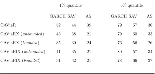
Panel B (Table 4.5) shows the number of models out of the 100 companies with a quantile loss ratio of less than 1 compared to the baseline. Comparing unconstrained with constrained models, there is minimal difference in the number of improved models. The only noticeable changes are the AS models at the 1% quantile for CAViaRX and the GARCH at the 1% quantile for CAViaRfX where there is improvement due to the use of the bounded score.
For example, the loss ratio for the CAViaRX unconstrained SAV models improves for 68 models compared to 48 models from the 5% to the 1% quantile. Panel C (Table 4.5) shows the number of models out of 100 companies that satisfy both the DQ test and a quantile loss ratio less than 1 compared to the baseline CAViaR. Despite this, there is a clear differentiation in model performance observed between the 1% quantile and 5% quantile groups.
There are more firms under the 1% quantile that meet both conditions compared to the 5% quantile calibration. In both panels comparing the 1% and 5% quantiles, we see that more models fall within the AE region at the 5% quantile than the 1% model for most model specifications. By proposing an estimator derived from a quantile regression of textual data on non-financial firms, we have demonstrated that there is a marginal improvement in VaR backtesting performance for CAViaR models at the 1% quantile level.
Possible extensions of this research could include reformulating the quantile regression so that the idiosyncratic element of returns is obtained differently (e.g. definition of an abnormal return versus the systemic market return) or the implementation of other variable selection methods to select the lexicon of choice words ( eg penalized quantile regression).
Outline of model specifications per company per rolling period
Backtesting aggregate results for all CAViaR models