université du québec`a montréal

Introduction

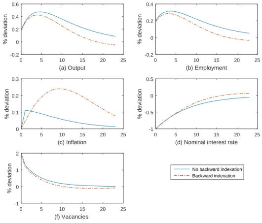
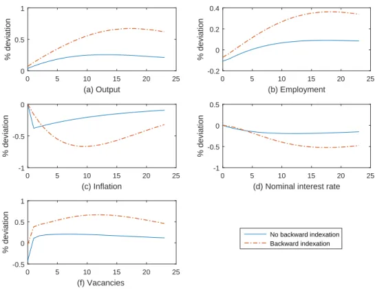
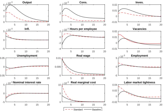
I further analyze the behavior of the model in relation to the effects of TFP shocks on output, employment, vacancies and inflation. First, reducing the degree of price stability increases the magnitude and peak effect of the inflation response in both models with and without indexation.

The Model

• The households
• The firms
• Monetary policy

1.9) The number of new jobs is given by the matching function in period t, M(ut, vt) = ζuξtv1−ξt, where ζ ∈ [0,1] covers the efficiency of the matching process, and ξ is the elasticity of matching. The unemployment rate is the number of workers who are not matched with the firm at the beginning of period t.

Calibration

To calculate the steady-state exogenous separation rate ρx, I follow the approach used in Den Han, Ramey, and Watson (2000). Following the approach of Walsh (2005), I assume that the log is normally distributed, serially uncorrelated, with standard deviation σa equal to 0.13.

Simulation results

• Impulse responses
• Comparative statistics

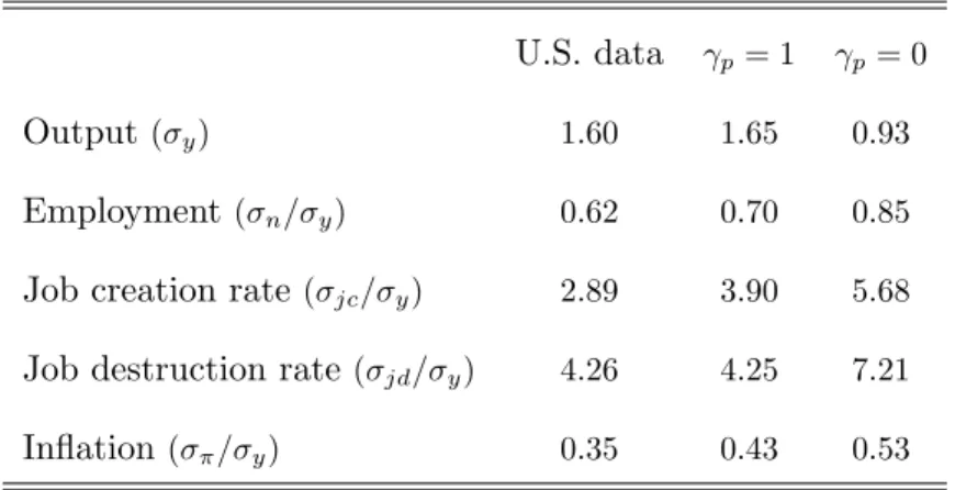
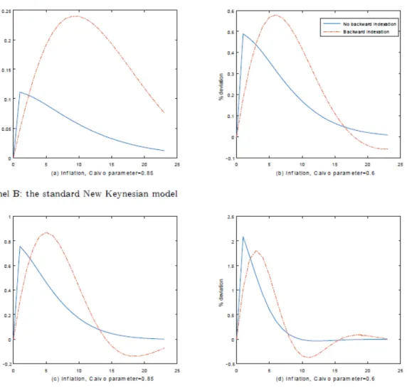
Set γp = 0 in the model without price indexation and γp = 1 in the model variant with indexation to past inflation. Again, the inflation response is more muted and less consistent in the model without lagged indexation.

The inflation dynamics

• Varying the degree of nominal rigidity
• Effects of search frictions

Panel A plots the response of inflation in the new Keynesian model with labor market search frictions. Panel B plots the response of inflation in the standard New Keynesian model without search frictions.

Conclusion

To measure vacancies (v), I use the help-wanted advertisement index, which is constructed by the Norwegian Conference Board.9 The labor market tightness variable (θ) is vu. With a fixed network, the model does a good job of capturing the simultaneous relationship between consumption and investment growth.7 The positive investment shock has two effects on consumption: a positive income effect and a negative substitution effect.

Introduction

The model is then able to capture the unemployment and labor market volatility observed in the data.1. Other solutions to the instability of the labor market problem include (i) assuming high elasticities of labor supply in real business models (Chetty, Guren, Manoli, and Weber 2013); and (ii) high substitution ratios (Hagedorn and Manovskii 2008). I estimate the contribution of the interaction between an investment shock and a positive inflation trend to labor market volatility.

Third, I study the contribution of each shock to the volatility of the labor market variables and the impact of adding a positive trend inflation rate on the impulse responses of key variables following these shocks. In this section, I quantitatively discuss the role of investment shocks and positive trend inflation in reproducing labor market volatility.

The Model

• The labor market
• Households
• The wholesale firms
• Workers
• Wage bargaining
• Retailers
• Monetary policy
• Aggregation

I set the labor force equal to one, so that utre also represents the unemployment rate and nt= 1−ut is the employment rate. Following Merz (1995), I use the assumption of a perfect insurance market, so that consumption is the same in all households regardless of their labor income due to their position in the labor market. Equation (2.17) states that the real rent is equal to the marginal productivity of capital.

Equation (2.18) describes the relationship between the marginal cost of announcing a vacancy, the probability of filling the vacancy and the value of the marginal worker in the next period t+ 1. 1 +R) ]ρRεRt, (2.35) where R is the nominal interest rate in the state of dynamic equilibrium, ρR ∈(0,1) captures the level of interest rate smoothing, φπ and φy are the non-negative coefficients of the policy rule and εRt is the i.i.d.

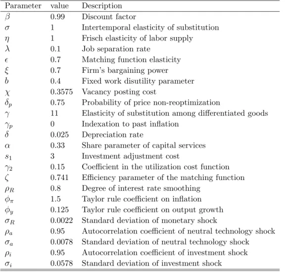
Calibration

I set the Calvo parameter, δp, equal to 0.75, which implies that firms keep their prices unchanged during 4 quarters. In the DSGE literature, there is some uncertainty about the duration of price contracts. Trigari (2009) sets the probability Calvo equal to 0.85 corresponding to an average duration of price rigidity of 6.5 quarters.

The elasticity of substitution between differentiated goods γ is 11, which corresponds to a steady-state price markup of 10 percent when the steady-state inflation rate π = 1. The standard deviation of the monetary shock, σR is set to 0.0022 which is standard in the literature.

Impulse responses

• Monetary policy shock
• Neutral technology shock
• Investment shock

Finally, trend inflation tends to increase the volatility and persistence of macroeconomic variables, especially for the labor market variables. Since the adjustment in total hours occurs at both the intensive and the extensive margins, hours per employee are slightly more responsive to moderate trend inflation. In this section, I study fluctuations in macroeconomic variables after an investment shock and assess the interaction between this shock and positive trend inflation to generate reinforcement.

In Figure 2.3, positive trend inflation increases the impact of an investment shock on inflation and increases price dispersion (not reported). The interaction between trend inflation and an investment shock has a larger effect on labor market variables than either TFP or monetary policy shocks.

Matching moments

• Labor market statistics in U.S. data
• Labor market statistics in the model

With no trend inflation, the model reproduces about 62 percent of the unemployment volatility observed in data. Again, adding the positive trend inflation rate into the model helps to reflect higher labor market volatility. For example, with positive trend inflation, the unemployment volatility relative to that of output generated by the model represents 19.5 percent of the observed value (see Table 2.5).

For example, a model with a positive trend accounts for about 60 percent of the observed volatility of unemployment relative to output (Table 2.5). Panel (v) in Table 2.6 shows that the zero-trend inflation model explains the standard deviation of the productivity variables (y/H) better than the positive-trend model (when ρi = 0.95).

Conclusion

Panel (ii) shows statistics for the model with only the neutral technology shock, while the standard deviations of the monetary and investment shocks are set to zero. The contribution of the neutral technology shock to the variance of output is about 25 percent. The second subsection reports the results for the Nash wage bargaining version of the model.

The standard deviation of the investment shockσi is 1.14 times smaller when there are fixed networks in the model. The correlation of the labor market variables with output growth in the baseline model increases.

Introduction

The use of firm networking is not new in dynamic stochastic general equilibrium (DSGE) models. I look at the interaction between business networking and the credible wage and its effects on labor market volatility and business cycle fluctuations in general. I find that without the integration of firms (standard model), the volatilities of key labor market variables are higher than in the US.

When upgrading the model to include firm networking (the base model), the unemployment volatility implied by the model matches that in the data. Finally, the presence of business networking helps account for the positive response of consumption in response to an investment shock1.

Model

• The labor market
• Households
• The wholesale firms
• Workers
• The alternating-offer wage bargain
• Comparison between the credible and the Nash wage determi-
• Retailers
• Monetary policy
• Aggregation

The total consumption is ct =. where γ is the elasticity of substitution between differentiated goods in retail firm j. The representative household enters period t with the stock of nominal bonds B and the physical capital Ktp. The household chooses the capital utilization rate Zt to convert the physical capital Ktpin into capital services, Kt = ZtKtp, and rents it to firms at the nominal rent Rkt. Company i posts job openings and pays the hiring costs χ to produce the differentiated wholesale good Xit that it sells to retail firms at the flexible price Pit. The discounted value of the company's future real profits is expressed as follows.

PtXitd−wit(hit)nit−Γit− χ. 3.15) HereXitd is the demand for the good produced by wholesale,wit(hit) = WitP(hit). Hit is the value of the marginal worker for firm i at period t given by Hit =mctmplthit−wt(hit) +Etβt,t+1(1−λ)Hit+1.

Calibration

The calibration of the intermediate input proportion φ comes from the definition presented by Nakamura and Steinsson (2010). To calculate standard deviations for the three shocks, I impose that the model matches the standard deviation of output growth observed in US estimates from Getler, Sala, and Trigari (2008) show that the investment shock explains about 54.8 percent of the variance decomposition of output growth rate.

The contribution of the other shocks to the variance of the output is about 20 percent. For the calibration of the standard deviations of all three shocks, I find that the investment shock accounts for 50 percent of the variance of output growth, the neutral technology shock 35 percent, and the monetary shock 15 percent.

Data

With the baseline model, I therefore get σa = 0.0050 for the standard deviation of the neutral technology shock, σr = 0.0037 for the standard deviation of the monetary shock and σi = 0.0437 for the investment shock. I set the autocorrelation coefficient of this shock to 0.95. I set the autoregressive parameter of the investment shock to 0.7, (Justiniano, Primiceri and Tambalotti, 2010).

Simulation results

• Model with CAOB wage
• Model with Nash wage bargaining
• Inflation persistence and impulse responses

The baseline model reproduces 78 percent and 83 percent of the observed volatility of consumption growth and investment growth, respectively. For example, the baseline model reproduces 76 percent of the variability of inflation relative to the variability of output growth observed in data, while the standard model overestimates this value by 42 percent. The effect of the monetary shock is magnified by the presence of firm networks with a standard deviation σr that is 1.4 times smaller than in the standard model.

The standard deviation of the neutral technology shock σa is 2.32 times smaller with the baseline model than with the standard model. This increases mainly due to the failure of the standard model to fit the variance of the labor market variables observed in data.

Conclusion

Note: This table shows the standard deviations of three shocks used in the model with firm networks (the basic model) and in the model without firm networks (the standard model). Note: This table shows the standard deviations of three shocks used in the model with firm networks (the base model) and the model without firm networks (the standard model). The column labeled “No FN, Nash” shows statistics for the model without firm networks and with Nash wage bargaining.

The column labeled “FN, Nash” shows statistics for the model with both firm networks and Nash wage bargaining. Note: This table shows statistics for autocorrelations of inflation at different lags for different versions of the model.

All equilibrium equations

• Impulse responses to a monetary shock
• Impulse responses to a productivity shock
• Effects of Calvo parameter on inflation
• Effects of search frictions on inflation in response to monetary shock 40
• Impulse responses to a neutral technology shock
• Impulse responses to investment shock
• Impulse responses to a monetary shock
• Impulse responses to a neutral technology shock
• Impulse responses to an investment shock
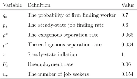
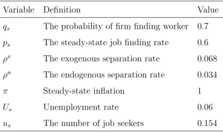
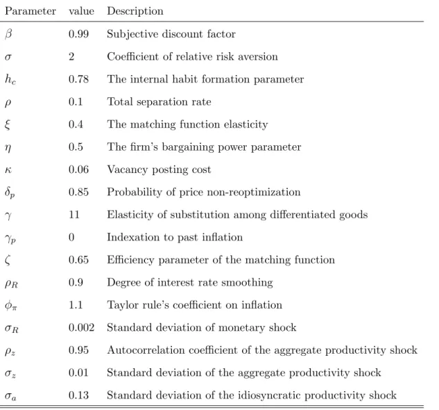
• Parameter values in the model with no price indexation
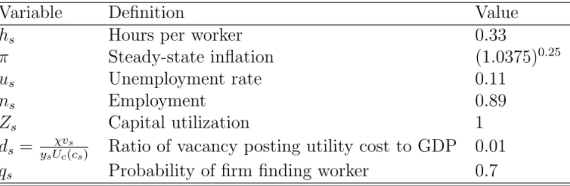
• Steady-state
• Effects of backward indexation on variables following a monetary
• Relative standard deviations
• Parameter values
• Steady-state
• Moments for model with and without positive trend inflation
• Volatility effects of trend inflation, shock sources (1)
• Volatility effects of trend inflation, shock sources (2)
• Volatility effects of trend inflation, shock sources (3)
• Parameter values for baseline model
• Steady state
• The size of shocks- Split (1)
• Moments in the baseline and the standard models- Split (1)
• The size of shocks in models- Split (2) and (3)
• Moments in the baseline and the standard models- Split (2) and (3) 122
• Moments in models with CAOB/Nash wages- Split (1)
• Inflation autocorrelations with CAOB wage- split (1)

Investment Shocks and the Barro-King Curse in New Keynesian Models.” National Bureau of Economic Research, Working Paper no. Monetary Policy, Trend Inflation, and the Great Moderation: An Alternative Explanation.” American Economic Review. Technology, Employment, and the Business Cycle: Do Technology Shocks Explain Aggregate Fluctuations?.” American Economic Review.

The Quantitative Importance of News Shocks in Estimated DSGE Models.” Journal of Money Credit and Banking. The (Ir)relevance of real wage rigidity in the new Keynesian model with search frictions." Journal of Monetary Economics.