Wage Bargaining, Search Frictions, and Firm Heterogeneity

IZA DP No. 3363

Globalization and Labor Market Outcomes: Wage Bargaining, Search Frictions, and Firm Heterogeneity

Julien Prat

Hans-Jörg Schmerer

DISCUSSION PAPER SERIES

Forschungsinstitut zur Zukunft der Arbeit Institute for the Study

February 2008

Globalization and Labor Market Outcomes: Wage Bargaining, Search

Frictions, and Firm Heterogeneity

Gabriel Felbermayr

University of Tübingen

Julien Prat

University of Vienna and IZA

Hans-Jörg Schmerer

University of Tübingen

Discussion Paper No. 3363 February 2008

IZA P.O. Box 7240

53072 Bonn Germany

Phone: +49-228-3894-0 Fax: +49-228-3894-180

E-mail: [email protected]

Any opinions expressed here are those of the author(s) and not those of IZA. Research published in this series may include views on policy, but the institute itself takes no institutional policy positions.

The Institute for the Study of Labor (IZA) in Bonn is a local and virtual international research center and a place of communication between science, politics and business. IZA is an independent nonprofit organization supported by Deutsche Post World Net. The center is associated with the University of Bonn and offers a stimulating research environment through its international network, workshops and conferences, data service, project support, research visits and doctoral program. IZA engages in (i) original and internationally competitive research in all fields of labor economics, (ii) development of policy concepts, and (iii) dissemination of research results and concepts to the interested public.

IZA Discussion Papers often represent preliminary work and are circulated to encourage discussion.

Citation of such a paper should account for its provisional character. A revised version may be

IZA Discussion Paper No. 3363 February 2008

ABSTRACT

Globalization and Labor Market Outcomes:

Wage Bargaining, Search Frictions, and Firm Heterogeneity

We introduce search unemployment à la Pissarides into Melitz’ (2003) model of trade with heterogeneous firms. We allow wages to be individually or collectively bargained and analytically solve for the equilibrium. We find that the selection effect of trade influences labor market outcomes. Trade liberalization lowers unemployment and raises real wages as long as it improves aggregate productivity net of transport costs. We show that this condition is likely to be met by a reduction in variable trade costs or the entry of new trading countries.

On the other hand, the gains from a reduction in fixed market access costs are more elusive.

Calibrating the model shows that the positive impact of trade openness on employment is significant when wages are bargained at the individual level but much smaller when wages are bargained at the collective level.

JEL Classification: F12, F15, F16

Keywords: trade liberalization, unemployment, search model, firm heterogeneity

Corresponding author:

Gabriel Felbermayr University of Tübingen Economics Department Nauklerstrasse 47 72074 Tübingen Germany

E-mail: [email protected]

* We are very grateful to Carl Davidson, Alan Deardorff, Hartmut Egger, Gino Gancia, Hugo Hopenhayn, Willi Kohler, Udo Kreickemeier, Omar Licandro, Marc Melitz, Gianmarco Ottaviano, Horst Raff, Rubén Segura-Cayuela, Jaume Ventura, as well as participants at the IAW anniversary conference, the 5^th ELSNIT Conference in Barcelona, and seminars at the Warsaw School of

1 Introduction

Public opinion meets globalization with mixed feelings. People agree that consumers benefit from trade but they are at the same time deeply concerned by its impact on job security. Fueled by numerous headlines about layoffs and outsourcing, many fear that globalization will worsen their prospects on the labor market.¹ To a certain extent, economic theory can rationalize this fear. Workers who lose their jobs due to trade liberalization have to go through a period of active search before finding new employment opportunities. During this period of transition, job reallocations increase the amount of frictions in the labor market which mechanically pushes up the rate of unemployment. On the other hand, comparatively little is known about the long-run effect of trade liberalization on unemployment. This is largely because equilibrium theories of trade and labor are still poorly integrated. In this paper, we attempt to bridge the two literatures by proposing a framework which combines the currently dominant approaches in each field.

We integrate a slightly generalized version of Melitz’s (2003) trade model with Pissarides’

(2000) canonical model of equilibrium unemployment. Building on Hopenhayn (1992) and Krug- man (1980), the Melitz-model shows how trade liberalization affects the productivity distribution of firms through selection of efficient firms into exporting and of inefficient firms into exit. That selection effect enjoys massive empirical support²and constitutes a tangible source of gains from trade that the earlier literature has paid little attention to. Our analysis suggests that it also matters for labor market outcomes. We find that, for reasonable parameter values, the cleans- ing effect of trade lowers search unemployment. As the cost of vacancy posting relative to the productivity of the average firm decreases, employers intensify their recruitment efforts. This raises the ratio of job vacancies to unemployed workers, which leads to lower unemployment and higher real wages.

Our framework generalizes Melitz’s and Pissarides’ set-ups as follows. First, we allow for a flexible parameterization of the external scale effect through which input diversity affects ag- gregate productivity. This helps to disentangle the selection effect from the diversity-enhancing effect of trade modeled by Krugman (1980). It also addresses recent empirical evidence by Arde- lean (2007) which puts the strength of the scale effect at a level substantially lower than the one implicitly assumed in the literature.³ We also need to adapt the search-matching framework,

1Scheve and Slaughter (2001) provide a detailed analysis of how American workers perceive globalization.

2See, among others, the surveys by Helpman (2006) or Bernard et al. (2007).

3Recent work by Corsettiet al. (2007) stresses the importance of external scale economies in a homogeneous-

which builds on competitive product markets, to make it compatible with the assumption of monopolistic competition used in trade models of the Krugman (1980) tradition. Allowing for monopoly power on product markets implies that we have to abandon matches as our unit of analysis and consider instead multiple-worker firms. Given the existence of search frictions, this introduces the complication of intra-firm bargaining. We analyze two environments: individual bargaining, where each worker is treated as the marginal worker and which is closest to com- petitive wage setting; and collective bargaining, where management bargains about wages and employment with firm-level unions.

Although the model features firms with heterogeneous productivity, monopoly power on product markets, external economies of scale, and, due to search frictions, monopsony power on labor markets, we are able to characterize its equilibrium in closed-form. The aggregation procedure proposed by Melitz goes through with little modification because, regardless of the bargaining environment, firms with different productivity levels pay similar wages. We also ob- tain a usefulseparability result according to which the equilibriumaverage productivity of input producers is independent from labor market outcomes. Accordingly, the system of equilibrium conditions turns out to be recursive. One can follow the same steps than Melitz (2003) to com- pute the average productivity in the economy and then solve for the equilibrium in the labor market.

In the absence of scale economies, the labor market equilibrium can be derived as in the stan- dard Mortensen-Pissarides model by interacting a job creation and a wage curve. Then, whether trade liberalization improves or worsens labor market outcomes depends solely on how it affects average productivity. Even though trade liberalization reallocates market shares towards effi- cient firms, exporters also incur transport costs that have to be deducted from the productivity gains. This is why trade liberalization does not necessarily enhance average productivity. We establish that both average productivity and employment always increase following a reduction in variable trade costs or an increase in the number of trade partners, as long as fixed foreign distribution costs are larger than domestic ones. Given that this requirement is satisfied by realistic calibrations of the model, such liberalization policies are likely to improve labor market outcomes. The gains of reducing fixed costs for foreign firms turn out to be more elusive because such a change benefits almost exclusively to new exporters.

Introducing external economies of scale drives a wedge between average and aggregate pro- ductivity. It complicates the analysis as we also have to take into account the positive rela-

firms, open macro model.

tionship between input diversity and aggregate productivity. This new effect gives rise to an additional equilibrium relation and restricts the parameter space where the model admits a unique equilibrium. Setting aside these technical results, we find that scale economies do not modify the qualitative implications of the model. They actually reinforce the positive impact of trade liberalization by adding the variety-enhancing effect described in Krugman (1980) to the selection effect.

We conclude our analysis by a calibration exercise. Simulating various trade liberalization scenarios allows us to to sort out the ambiguities, in particular regarding the role of fixed foreign costs, and to assess the magnitude of the effects. The simulations predict that reducing variable trade costs, or increasing the number of trade partners, has a significantly positive impact on both wages and employment. The labor market effects of trade liberalization are strongly conditioned by the nature of the wage bargaining environment. When wages are negotiated collectively rather then individually, trade reform yields substantially lower unemployment gains, with aggregate productivity gains almost entirely absorbed by rising real wages. Moreover, results are sensitive with respect to the size of external scale economies; this calls for more empirical research into the parameters governing the model.

Related literature. This paper builds on our earlier work (Felbermayr and Prat, 2007) where we introduce search unemployment into a closed economy version of Melitz (2003) with the aim to study product market regulation. The relation to the present paper is straightforward, since trade liberalization can be understood as an alternative type of product market reform.

In modeling bargaining regimes, we draw on Ebell and Haefke (2006), who analyze a closed- economy, homogeneous firms model of search and unemployment.

There is a growing number of theory papers on the trade-unemployment relationship with heterogeneous firms. Our approach is closely related to the recent work of Egger and Kreick- emeier (2007), who study the effect of trade liberalization in a model with fair wages. They find that trade increases the wage dispersion among identical workers and also leads to more unemployment. Davis and Harrigan (2007) find similar results for the degree of wage dispersion and unemployment, using an efficiency wages approach instead of fair wages.

There is a small but important literature onsearch unemployment in Heckscher-Ohlin trade models which goes back to Davidson et al. (1988). Building on this seminal line of research, three recent papers also discuss search unemployment in trade models with heterogeneous firms.

The model closest to ours is presented by Janiak (2006). His framework exhibits an equilibrium

under the assumption that the elasticity of substitution is smaller than two. As explained below, this restriction explains why Janiak’s model predicts that trade liberalization raises equilibrium unemployment. In our model, equilibrium existence and uniqueness is guaranteed under less restrictive and more plausible conditions.

Mitra and Ranjan (2007) and Helpman and Itskhoki (2007) introduce search unemployment in two-sector models with heterogeneous firms. Their papers differ from ours in terms of mo- tivation and setup: Mitra and Ranjan discuss the role of off-shoring; Helpman and Itskhoki focus on how labor market distortions diffuse internationally through trade. In contrast to our paper, Helpman and Itskhoki deviate from the standard search-and-matching framework as they disallow for forward-looking behavior of workers and firms on the labor market. Moreover, the symmetric version of their model (which is most easily comparable to our setup) features a neg- ative trade-unemployment link: trade boosts average productivity in the differentiated goods sector, making employment there more attractive. This leads to a reallocation of labor from the distortion-free num´eraire sector into the friction-ridden differentiated goods sector.⁴

Structure of the paper. The remainder of the paper is organized as follows. Section 2 lays-out the set-up of the model. In section 3, we analyze two ways of endogenizing wages:

individual bargaining and efficient collective bargaining. In section 4, we describe exit and entry of firms. Section 5 studies the effects of three globalization scenarios: (i) a reduction in variable trade costs, (ii) an increase in the number of trade relations, (iii) a reduction in fixed exporting costs. Section 6 calibrates the model in order to quantify the magnitude of the effects. Section 7 concludes. Proofs of the propositions, lemmata and corollaries are included in the Appendix.

2 Setup of the Model

We consider an economy that is essentially similar to the one analyzed in Melitz (2003) but for the existence of search frictions in the labor market. As in Melitz, the world is modeled as a collection of symmetric countries which interact on product markets.⁵ We deviate from existing treatments by explicitly parameterizing the external effect of increased input diversity on aggregate productivity.

4Davidson et al. (2007) propose a model with two-sided heterogeneity, where goods markets are perfectly competitive and firms endogenously choose technologies.

5For brevity, we skip the special case of autarky. Due to symmetry, we do not use country indices.

Final output producers. The setup of the production side of our model is akin to Egger and Kreickemeier (2007). The single final output good, Y, is produced under conditions of perfect competition and can be either consumed or used as an input in the production process. Good Y is assembled from a continuum of intermediate inputs, which may be produced domestically or imported, and which may command different equilibrium prices. Denoting the quantity of such an input q(ω), we posit the following production function

Y =

M^ν−1σ Z

ω∈Ω

q(ω)^σ−1σ dω _σ−1^σ

, σ >1, ν∈[0,1], (1) where the measure of the set Ω is the mass M of available intermediate inputs, each produced by a monopolistically competitive firm. We refer to M as the degree ofinput diversity while σ denotes the elasticity of substitution between any two varieties of inputs.

To understand the role played by ν, suppose that all varieties are demanded in identical quantities. Substituting q(ω) = Q/M, where Q is an aggregate index of input demand, yields Y =M^σ−1ν Q. If ν = 0,thenY =Q and the number of available varieties is irrelevant for total output. This is the case discussed by Giavazzi and Blanchard (2003) or Egger and Kreickemeier (2007).⁶ If ν = 1,the production function takes the conventional Dixit-Stiglitz form, where an increased number of varieties increases total output.

Specification (1) offers at least three advantages. First, the recent estimates of Ardelean (2007) indicate that ν ∈ (0,1). Hence, the conventional formulation where ν = 1 tends to exaggerate the role of diversity for aggregate productivity. Second, ifν >0,the autarky version of our model yields a counterfactual negative correlation between the unemployment rate and the labor supply. With trade and symmetric countries, this counterfactual implication is maintained on the world level.⁷ We nonetheless allow for ν >0 to accommodate the dominant practice in the trade literature where gains from increased diversity are generally deemed important. Third, equation (1) withν = 1 yields the cases discussed by Krugman (1980) or Melitz (2003) and thus allows us to address the importance of this assumption for their results.

The price index dual to (1) is P =

M^ν−1R

ω∈Ωp(ω)^1−σdω1/(1−σ)

, wherep(ω) is the price

6Our formulation of the aggregate production is formally similar to the utility function employed by Corsetti, Martin, and Pesenti (2007) who also stress the role of ν. Egger and Kreickemeier (2007) allow forν ∈[0,1] in the appendix of their paper. Benassy (1996) discusses how the welfare properties of the Krugman (1980) model depend onν.In particular, ifν6= 1,the decentralized equilibrium may yield over- or under-supply of input variety.

This discussion carries over to the Melitz (2003) model.

7With heterogeneous countries and costly trade, larger countries suffer less from trade costs, have a higher level of aggregate productivity, and a lower rate of unemployment.

of inputω,inclusive of potential trade costs. We choose the final output good as thenum´eraire, i.e. P = 1.Then the demand of intermediate inputs ω reads

q(ω) = Y

M^1−νp(ω)^−σ. (2)

Intermediate input producers. At the intermediate inputs level, there is a continuum of monopolistically competitive firms which produce each a unique variety. Labor is the unique fac- tor of production. It is inelastically supplied by the household and enters firms’ production func- tions linearly. Firms have different productivity levels ϕ(ω), so that output q(ω) =l(ω)ϕ(ω).

In the following, we use ϕto index intermediate input producers.

On the domestic and on each of the n symmetric export markets, input producers face fixed market access costs (e.g., distribution costs), f_D and f_X respectively.⁸ We assume that τ^σ−1fX > fD. As explained below, this ensures that only a subset of firms export and that exporters are on average more efficient than non-exporting firms.

International trade is subject to the traditional variable iceberg trade costsτ ≥1.In order to deliver a unit of input to a foreign market, the firm has to manufacture τ units. If it decides to serve both the domestic and the foreign markets, a firm allocates its output so as to maximize its total revenues. Operating revenues from sales on a given foreign market are therefore equal topXqX/τ.⁹ By symmetry, demands on the domestic and foreign markets are given by equation (2). Equating marginal revenues across markets therefore yieldsp_X(ϕ) =τ p_D(ϕ) and q_X(ϕ) = τ^1−σqD(ϕ), whereD and X denote the domestic and the export market. Hence, total revenues are given by

R(l;ϕ)≡ Y

M^1−ν 1 +I(ϕ)nτ^1−σ 1/σ

(ϕl)^σ−1σ , (3)

with I(ϕ) being an indicator function that takes value one when a ϕ-firm exports and zero otherwise. Apart from the fact that their effective demand level is multiplied by 1 +nτ^1−σ, exporting firms have similar revenue functions than non-exporting firms.

In order to facilitate the aggregation procedure, we define the average productivity level ϕe such thatqD(ϕ) =e Y /M^{σ−1ν +1}. In the benchmark case where there are no externalities of scale, so thatν = 0,the domestic salesq_D(ϕ) of the average firm is equal to the average sales per firme

8Since capital markets are perfect and uncertainty is resolved before market access costs are paid, fX and fD can be thought as flow fixed costs or – appropriately discounted – as upfront investment. In the latter case, whenever applicable, we use upper-case letters.

9Notice thatpX is the c.i.f. price in the foreign market.

Y /M, and the domestic price of its goodp_D(ϕ) =e P = 1.

Search frictions. The labor market is imperfectly competitive due to the existence of search frictions. Whereas marginal recruitment costs are increasing at the aggregate level because of congestion externalities, they are exogenous from a firm’s point of view. The aggregate matching function is homogeneous of degree one so that the vacancy-unemployment ratio θ uniquely determines the rate m(θ) at which firms fill their vacancies. That rate is a decreasing function of θ and satisfies the following standard properties: limθ→∞m(θ) = 0 and limθ→0m(θ) = ∞.

Due to the linear homogeneity of the matching function, job seekers meet firms at the rateθm(θ) which is increasing in θ. The cost of posting vacancies is proportional to the parameter c, so that recruiting l workers entails spending [c/m(θ)]l. In other words, firms face an adjustment cost function that is linear in labor.

3 Labor Market Equilibrium

This section characterizes the labor market equilibrium for two common models of wage de- termination, individual and collective bargaining. We establish that, in both cases, wages are constant across firms and the vacancy-unemployment ratio is increasing in aggregate productiv- ity. In the subsequent analysis, we will index endogenous variables by the subscript I orC to indicate individual or collective bargaining.¹⁰

We devise our model in discrete time. All payments are made at the end of each period.

Before the beginning of the next period, firms and workers are hit by idiosyncratic shocks: (i) with probability δ, intermediate producers are forced to leave the market; (ii) with probability χ, each job is destroyed because of match-specific shocks. We assume that these two shocks are independent so that s=δ+χ−δχ denotes the actual rate of job separation.

Unemployed workers earn a flow income of bΦ, where Φ ≡ M^σ−1ν ϕ˜ measures aggregate productivity (while–with some abuse of wording–we refer to ˜ϕasaverageproductivity). Indexing the value of non-market activity to Φ is consistent with the empirically relevant case where unemployment benefits are proportional to aggregate productivity.¹¹ In any case, when ν = 0, setting the flow value of non-market activity equal to an exogenous constant does not affect

10We drop these indices when there is no risk of confusion.

11Directly indexing the value of non-market activity to wages, i.e. assuming that unemployed workers earn a flow income equal tobwwithb <1, yields similar results but slightly complicates the algebra.

our main insights. On the other hand, when there are economies of scales (ν > 0), it leads to multiple equilibria while our normalization ensures the existence of a unique equilibrium.

3.1 Individual wage bargaining

Individual wage bargaining involves the following sequence of actions: at each period, the inter- mediate input producer decides about the optimal number of vacanciesvI,taking the wage rate as given. The matching technology brings together the workers and the firm. Before production takes place, wages are bargained. Wage contracts are unenforceable: at any point in time, the firm may fire any employee and symmetrically any employee may quit. Solving the game by backward induction, we first characterize the firm’s optimal vacancy setting behavior, and then solve the bargaining problem.

The market value of an intermediate producer solves J_I(l_I;ϕ) = max

vI

1 1 +r

R(l_I;ϕ)−w_I(l_I;ϕ)l_I−cv_I−f_D−I(ϕ)nf_X + (1−δ)J_I l⁰_I;ϕ , (4) s.t.(i)R(lI;ϕ) =

Y

M^ν−1 1 +I(ϕ)nτ^1−σ 1/σ

(ϕlI)^σ−1σ , (ii)l⁰_I = (1−χ)lI+m(θI)vI,

where l⁰_I is the level of employment next period, and the dependence of l_I, v_I and q_I on ϕ is understood. Constraint (i) is the revenue function (3) and (ii) gives the law of motion of employment at the firm level. The first order condition for vacancy posting reads

c

m(θ_I) = (1−δ)∂JI(l⁰_I, ϕ)

∂l⁰_I , (5)

so that the firm sets the shadow value of labor equal to the marginal recruitment cost. Substi- tuting the constraints into the objective function of the firm, differentiating with respect to l_I, and using the optimality condition (5) yields

∂J_I(l_I, ϕ)

∂l_I = 1 1 +r

∂R(l_I;ϕ)

∂l_I −w_I(l_I, ϕ)−∂w_I(l_I, ϕ)

∂l_I l_I+ c

m(θ_I)(1−χ)

. (6)

The firm acts as a monopsonist by taking into account the effect of additional employment on the wage of inframarginal employees. Replacing the first order condition (5) on the left-hand side of (6), we obtain an expression that implicitly determines the optimal pricing behavior of the monopolist

∂R(l_I;ϕ)

∂lI

=w_I(l_I, ϕ) +∂w_I(l_I, ϕ)

∂lI

l_I+ c m(θI)

r+s 1−δ

. (7)

This expression differs from Melitz (2003) in that marginal costs are augmented by a monopsony effect and expected recruitment costs.

The total surplus accruing from a successful match is split between the employee and the firm.

The worker’s surplus is equal to the difference between the value of being employed E_I(l;ϕ) by a firm with productivity ϕ and workforce l and the value of being unemployed U_I. The firm’s surplus is simply equal to the marginal increase in the firm’s value∂JI(l;ϕ)/∂lI because individual bargaining implies that each employee is treated as the marginal worker. Following Stole and Zwiebel (1996) we assume that the outcome of bargaining over the division of the total surplus from the match satisfies the following “surplus-splitting” rule

(1−β) [EI(l;ϕ)−UI] =β∂JI(l;ϕ)

∂lI

, (8)

where the parameterβ measures the bargaining power of the worker and thus belongs to (0,1).

As explained by Stole and Zwiebel (1996), condition (8) can be micro-founded either by cooperative or non-cooperative game theory. In the non-cooperative case, condition (8) charac- terizes the unique subgame perfect equilibrium of an extensive form game where the firm and its employees play a bargaining game of Binmore et al. (1986) within each bargaining session.

Accordingly, neither the firm nor any employee can improve their positions by renegotiating.

In the cooperative case, condition (8) assigns to each party its Shapley value, that is the av- erage, over all possible permutations, of each player contribution to possible coalitions ordered below him.¹² When β differs from 1/2, condition (8) generalizes the symmetric Shapley value to situations where players are not treated identically.

Using the shadow value of labor (6) in the bargaining solution (8), we obtain a differential equation in the wage rate, which can be solved to give rise to aWage curve (W_I). The equilib- rium wage and labor market tightness are found by interacting W_I with a Job Creation curve (J CI), as in standard search-matching models.

Proposition 1 When wages are bargained at the individual level, the labor market admits an equilibrium if and only if b < _σ−β^σ−1. The equilibrium is unique and such that wages are constant across firms. The equilibrium wage, wI, and vacancy-unemployment ratio, θI, simultaneously

12This interpretation is the one favored by Helpman and Itskhoki (2007).

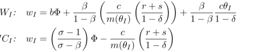
satisfy the following Wage and Job Creation conditions:

W_I: w_I =bΦ + β 1−β

c m(θ_I)

r+s 1−δ

+ β

1−β cθ_I

1−δ (9)

J C_I: w_I =

σ−1 σ−β

Φ− c

m(θI)

r+s 1−δ

(10) The Job Creation curve characterizes firms’ optimal recruitment efforts which are, as ex- pected, decreasing in the wage level. The Wage curve implies that wages depend only on aggregate productivity so that workers are paid similarly across firms with different productivity levels. This somewhat surprising result extends to a dynamic setting the proof of Stole and Zwiebel (1996) that firms exploit their monopsony power until employees are paid their outside option. In our case, the outside option is augmented by the recruitment costs that the firm would have to pay if it were to replace the worker. Quite intuitively, the workers’ bargaining position is improving in the severity of labor market frictions which explains why the Wage curve is increasing in θ.

The existence condition in Proposition 1 states that the flow value of non-market activity should not yield revenues in excess of a share (σ−1)/(σ−β) of aggregate productivity. For values of σ above 2 and bargaining power β close or below 1/2, as commonly assumed in the literature, this implies that the flow value of non-market activity is no larger than 2/3 aggregate productivity; this is a rather undemanding requirement.

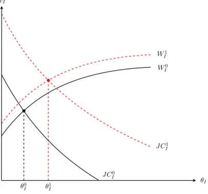
Figure 1 illustrates the effect of an increase in aggregate productivity Φ on labor market tightness. The Job Creation curve shifts upwards (from the solid to the dashed curve) because firms are on average more productive and search more intensively for workers. The intercept of the Wage curve also increases because unemployment benefits are proportional to aggregate productivity. However, this second effect is dominated because the flow value of non-market activity is only equal to a share b <1 of market productivity.¹³ Hence labor market tightness goes from θ_I⁰ to θ¹_I. Trade liberalization will affect labor market outcomes to the extent that it changes aggregate productivity Φ by modifying the degree of input diversity M and/or the average productivity of input producers ˜ϕ.

Corollary 1 When wages are bargained at the individual level, the vacancy-unemployment ratio θI is increasing in aggregate productivity Φ.

13When the flow value of non-market activity is simply set equal to an exogenous constant, the Wage curve is not affected by a change in ΦI. Then the result in Corollary1follows immediately.

θI

θ_I¹ θ⁰_I wI

W_I¹ W_I⁰

JC_I¹ JC_I⁰

1

Figure 1: Effect of an increasing Φ_I in the Individual Bargaining regime.

3.2 Collective bargaining

In a firm covered by collective bargaining, workers form a firm-wide coalition, that is, a trade union. When bargaining fails and workers go on strike, the firm loses not only the value associ- ated to the marginal worker, as with individual bargaining, but its entire labor force. We opt for an efficient bargaining setup so that the firm and the union bargain about both wages and employment. This ensures that we are considering equilibria lying on the Pareto frontier.¹⁴

Negotiations between the union and the firm take place in the first period.¹⁵ The union’s objective is the expected sum of its members’ rents

U(l, w)≡(1−δ)l

w−rU r+δ

,

14Our main results also hold in aright to manage set-up where unions negotiate only about wages and firms have full freedom to set the level of employment. Barth and Zweim¨uller (1995) study different wage bargaining scenarios when firms are heterogeneous with respect to their productivity.

15One could instead consider that the firm and the union bargain on the steady-state profits, so thatF(l, w;ϕ) = 1−δ

r+δ

h

R(l;ϕ)−wl(ϕ)−_m(θ)^c χl(ϕ)i

. This obviously generates a hold-up problem where the union does not take into account the initial recruitment costs. Then employment is lower and wages higher but the main insights of this section are not fundamentally modified.

while the firm seeks to maximize its expected variable profits F(l, w;ϕ)≡

1−δ

r+δ R(l;ϕ)−wl(ϕ)− c

m(θ)χl(ϕ)

− c m(θ_C)l .

The negotiation specifies both employment and wages. The solution lies on the contract curve which connects the points where the firm iso-profit curves are tangent to the union indifference curves. The actual agreement is pinned down by the union’s bargaining power β. Proposition 2 shows that the labor market equilibrium can be characterized in a similar fashion than in the Individual Bargaining regime.

Proposition 2 When wages are collectively bargained, the labor market admits an equilibrium if and only if b <(σ−1)/σ. The equilibrium is unique and such that wages are constant across firms. The equilibrium wage, w_C, and vacancy-unemployment ratio, θ_C, simultaneously satisfy the following Wage and Job Creation conditions:

WC: wC =bΦ +β σ

θCm(θC) r+s

Φ + β

σΦ (11)

J CC: wC =

1−1−β σ

Φ− c

m(θ_C)

r+s 1−δ

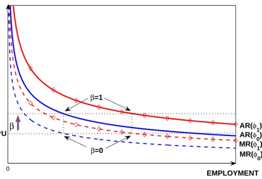
(12) For the same reasons than before, the Wage curve is increasing inθwhile the Job Creation curve is decreasing. The bargained wage is equal to the opportunity cost of employment rU_C plus a share β of the remaining profits per worker. Due to the existence of rent-sharing, and in contrast to individual bargaining, the slope of the Wage curve is increasing in aggregate productivity. Yet, as with individual bargaining, the wage rate is the same across firms with different levels of productivity. Figure 2 illustrates why, in our CES setting, differences in idiosyncratic productivity wash out so that there is no wage dispersion.

First consider the curves without dot. The plain curve plots the average revenues per worker while the dashed curve plots the marginal revenues. The competitive outcome where β = 0 is obviously given by the point where the marginal revenue function intersects the workers’ outside option rU_C. Starting from this point, the contract curve describes a vertical¹⁶ segment which reaches the average revenue function. This upper-bound gives the outcome when workers have all the bargaining power (β = 1) since then the firm’s profits net of fixed costs are zero. Whenβ varies between 0 and 1, wages fluctuate between these two extremes. Now consider the problem

16As usual, the verticality of the contract curve follows from the risk neutrality of workers. Introducing risk aversion yields a contract curve with a positive but bounded slope.

0 EMPLOYMENT rU

MR(φ₀) MR(φ₁) AR(φ₀) AR(φ₁) β=0

β=1

β

Figure 2: Collective bargaining withϕ₀< ϕ₁.

of a firm with a higher productivityϕ1 > ϕ0. As shown by the dotted curves, the only difference is that both average and marginal revenues functions are shifted to the right. Furthermore, since firms apply the same mark-up, the two curves are shifted parallely. Accordingly, firms with a higher productivity hire more workers but pay the same wage.

The most significant difference with the individual bargaining regime is that now aggregate productivity Φ also raises the slope of the Wage curve. Yet, as stated in Corollary 2, this additional effect on the Wage curve is again unambiguously dominated by the shift of the Job Creation curve.

Corollary 2 When wages are collectively bargained, the vacancy-unemployment ratioθ_C is in- creasing in aggregate productivity Φ.

We would like to acknowledge an important caveat before closing our characterization of the labor market: if search costs c were measured in units of labor, then increasing Φ would raise the real wage but leave the labor market tightness unchanged.¹⁷ This illustrates that changes

17Similarly, ifcwere indexed to aggregate productivity (e.g. c = Φ¯c, with ¯c >0) the equilibrium value of θ

in employment are driven by the negative effect of aggregate productivity on real vacancy costs.

For two reasons we stick to the assumption that vacancy costs are measured in units of the final output good. First, as soon as search costs depend on the price of the final output good (e.g.

c=w¯c+c, with{¯c, c} ⊂R²₊), variations in Φ do affectθso that Corollaries1and2continue to hold. Second, it is not clear how to model wage bargaining when the cost of a vacancy is itself subject to negotiation, as it would be the case if the production of search services were to draw on labor. We therefore stick to the conventional practice and assume that the search process does not directly require the use of labor.¹⁸

In this section, we have described how to solve for the labor market equilibrium. Our two equilibrium conditions take the average productivity, ˜ϕ, and the equilibrium diversity of inputs, M, as given. Changes in these two variables affect aggregate productivity Φ, thereby moving the Job Creation and Wage curves. To the extent that Φ goes up, the rate of unemployment falls and the real wage rises, regardless of the bargaining regime. The next section explains how to endogenize average productivity.

4 Firm Entry and Exit

We model firm entry and exit in a similar fashion than Melitz (2003), which in turn draws on the seminal work by Hopenhayn (1992). We deliberately keep the analysis as brief as possible and refer the reader to Melitz’ paper for further details. Our contribution is to show that the equilibrium level of average productivity ˜ϕ and the labor market tightness θ are independent (hence we drop subindices {I, C}from the outset).

The entry process is in two stages. First, prospective entrants pay an entry costF_E. Only after entering are they able to draw their productivity from a sampling distribution with c.d.f.

G(ϕ) and p.d.f. g(ϕ). After the draw, productivities remain constant over time.¹⁹ Given that firms’ revenues are increasing in ϕ, one can define a threshold ϕ^∗_D below which firms do not take up production. Similarly, firms with a productivity level between ϕ^∗_D and ϕ^∗_X will serve only their domestic market. The share of exporting firms is therefore equal to % ≡ [1−G(ϕ^∗_X)]/[1−G(ϕ^∗_D)]. The average level of productivity of intermediate input producers

would be independent from Φ.

18Note that, if aggregate TFP were trending, our model would always exhibit a balanced growth path, regardless of whether we indexcto Φ,wor to the final output good.

19This stylized assumption is made mainly for tractability reasons. It is the key difference between Melitz’s (2003) and Hopenhayn’s (1992) models, as the latter also allows firms’ productivities to vary over time.

is given by the following weighted sum

˜ ϕ=

( 1 1 +n%

"

˜

ϕ^σ−1_D +n%

ϕ˜X

τ

σ−1#)_σ−1¹

, (13)

where ˜ϕD and ˜ϕX are average productivity indices for the populations of firms that sell only domestically and that also sell abroad

˜

ϕ(ϕ^∗_D) =



 R+∞

ϕ^∗_D ϕ^σ−1g(ϕ)dϕ 1−G ϕ^∗_D





1 σ−1

and ˜ϕ(ϕ^∗_X) =



 R+∞

ϕ^∗_X ϕ^σ−1g(ϕ)dϕ 1−G ϕ^∗_X





1 σ−1

. (14)

Let us first characterize the entry thresholdϕ^∗_D. The linearity of the adjustment cost function implies that firms reach their optimal size by the end of their first period of activity.²⁰ It is profitable to start operating and to recruit workers when

(1−δ)

∞

X

t=0

(1−r−δ)^tπ_D(ϕ)− c

m(θ)l_D(ϕ)−f_D = (1−δ)πD(ϕ) r+δ − c

m(θ)l_D(ϕ)−f_D ≥0, (15) where

πD(ϕ) =pD(ϕ)ϕlD(ϕ)−wlD(ϕ)− c

m(θ)χlD(ϕ)−fD

is the optimal flow profit from domestic sales of a ϕ-firm. Condition (15) accounts for the fact that firms pay market access and vacancy costs up front but have to wait one period to recruit their workers. In this period, they can be hit by a destruction shock, so that, with probability δ, they never start producing. The cut-off productivity ϕ^∗_D is such that the weak inequality in (15) binds. The proportionality of domestic prices allows us to relate operating profits of the marginal and average firm

π_D( ˜ϕ_D) +f_D π_D ϕ^∗_D

+f_D = l_D( ˜ϕ_D) l_D ϕ^∗_D =

ϕ˜_D ϕ^∗_D

σ−1

.

Hence, (15) is equivalent to the followingZero Cutoff Profit condition πD( ˜ϕD) =

r+δ 1−δ

c

m(θ)lD( ˜ϕD)

+fD

"

ϕ˜D

ϕ^∗_D

σ−1 1 +r 1−δ

−1

#

. (16)

20Gradual convergence can be restored either by considering that recruitment costs are convex in the number of posted vacancies, as in Bertola and Caballero (1994), or by assuming that firms can post only one vacancy, as in Acemoglu and Hawkins (2007). Since this greatly complicates the aggregation procedure, we adopt a more parsimonious specification where, as in Melitz (2003), firms jump to their optimal size. See Koeniger and Prat (2007) for a numerical analysis of a model with firm entry and convex adjustment costs.

The choice of exporting status can be characterized in a similar fashion. One simply has to replace the subscriptsDin equation (15) byX and to update the definition of profits as follows

πX(ϕ) =pX(ϕ)ϕlX(ϕ)/τ −wlX(ϕ)− c

m(θ)χlX(ϕ)−fX .

Given that export prices are also proportional to productivity, we obtain a similar Zero Cutoff Profit (ZCP) condition for exporting firms

π_X( ˜ϕ_X) =

r+δ 1−δ

c

m(θ)l_X( ˜ϕ_X)

+f_X

"

ϕ˜_X ϕ^∗_X

σ−1 1 +r 1−δ

−1

#

. (17)

To see that some firms serve solely their domestic market, notice thatRX(ϕ) =pX(ϕ)qX(ϕ)/τ = τ^1−σR_D(ϕ) andl_X(ϕ) =τ^1−σl_D(ϕ). Accordingly, the flow profits satisfyπ_X(ϕ) =τ^1−σ[π_D(ϕ) + fD]−fX. Replacing this expression in (15) illustrates that aϕ^∗_D-firm does not find it profitable to incur the exporting costs when, as assumed in Section 2, τ^σ−1f_X > f_D.²¹

The ZCP conditions characterize the optimal decision of a firm who knows its idiosyncratic productivity. Free Entry(FE) allows us to take into account the behavior of prospective entrants.

Entry occurs until expected profits are equal to the entry cost FE, so that FE

1−G(ϕ^∗_D) = πD( ˜ϕD)

r+δ (1−δ)− c

m(θ)lD( ˜ϕD)−fD+n%

πX( ˜ϕX)

r+δ (1−δ)− c

m(θ)lX( ˜ϕX)−fX

. (18) Free entry holds when this equality is satisfied because an entrant will start to operate with probability 1−G(ϕ^∗_D). On the domestic market, successful entrants earn an average expected stream of profits equal to equation (15) as evaluated for the representative firm ˜ϕ_D. Moreover, entrants will also export with probability 1−G(ϕ^∗_X) = %[1−G(ϕ^∗_D)] and earn the average expected stream of profits on the export markets. Taking into account these two eventualities leads to equation (18). Combining the FE and ZCP Conditions yields

F_E = [1−G(ϕ^∗_D)]

1 +r r+δ

( f_D

"

ϕ(ϕ˜ ^∗_D) ϕ^∗_D

σ−1

−1

#

+n%f_X

"

ϕ(ϕ˜ ^∗_X) ϕ^∗_X

σ−1

−1

#)

. (19)

Although (19) depends on bothϕ^∗_D andϕ^∗_X, it actually pins down the two variables because ϕ^∗_X = ϕ^∗_Dτ(fX/fD)^σ−11 .²² Given that our equilibrium condition is the same than in Melitz

21When this partitioning does not hold, one cannot use equation (15) to determine whether or not a firm operates on the domestic market because it may be optimal to pay the fixed operating costfX in order to access the export markets.

22See the proof of Lemma1for a derivation of this equality.

(2003), the existence and uniqueness of the equilibrium in the product market are ensured. Most interestingly, the vacancy-unemployment ratioθdrops out when the FE and ZCP Conditions are interacted. This implies that, as stated in the following lemma, the entry and export thresholds depend solely on the product market parameters {F_E, fD, fX, n, τ, σ, r, δ}and the properties of the c.d.f. G(ϕ).

Lemma 1 (Separability)Regardless of the bargaining regime, the equilibrium average produc- tivity of intermediate producers, ϕ, does not depend on the vacancy-unemployment ratio˜ θor on input diversity M.

In other words, labor market conditions do not influence the optimal partitioning of firms.

Note that this is a general feature of the Melitz (2003) framework when firms pay identical wages.

To understand this result, it is useful to remember that the FE and ZCP conditions relate the average profit per firm to the cutoff productivity. Hence, they are not affected by the impact on operating revenues of changes in labor market tightness and wages. Firms’ equilibrium sizes adjust so as to offset any increase or decrease in revenues per worker until both product market conditions are satisfied again.

Accordingly, the only relevant effect is the positive relationship between θ and the initial recruitment costs, cl(ϕ)/m(θ), of newly created firms. On the one hand, higher recruitment costs discourage potential entrants. For a given level of operating profits, free entry requires a greater likelihood of entering the market, that is a lower cutoff productivity ϕ^∗. On the other hand, firms that have already paid the entry cost and have drawn their idiosyncratic productivity find it less attractive to initiate production when recruitment costs are higher. This obviously raises the cutoff productivity ϕ^∗. Given that the expected recruitment costs before entry are equal to the recruitment costs of the average firm, the ex-ante and ex-post effects of θ exactly offset each other.²³ Plotting, as Melitz (2003) does, the equilibrium conditions in the cutoff- productivity / average-profit space yields the following adjustments: following an increase in θ, both FE and ZCP loci shift up by the same amount so that the average profit per firm goes up, but the cutoff productivity remains constant.

The separability property stated in Lemma 1 allows to solve for equilibrium in a recursive way. Average productivity and cutoff productivities can be determined as in Melitz (2003) by considering solely product market parameters. Taking these values as given, we can then solve

23This property hinges on the log-linearity of firm sizes with respect toϕ. Hence, the independence ofϕ^∗onθ clearly depends on the CES specification.

for the equilibrium in the labor market. Note, however, that we still need to determine input diversityM in order to derive aggregate productivity Φ. As shown in the next section, this last step is trivial when there are no economies of scale but otherwise leads to the introduction of an additional equilibrium condition.

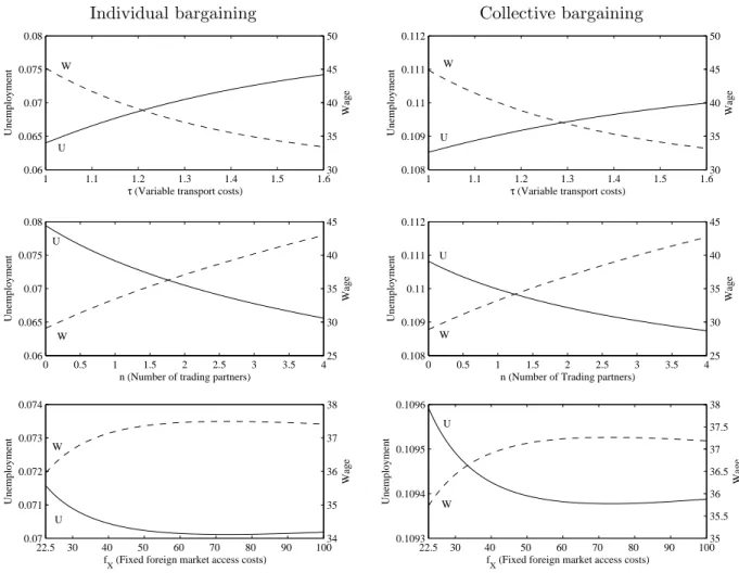
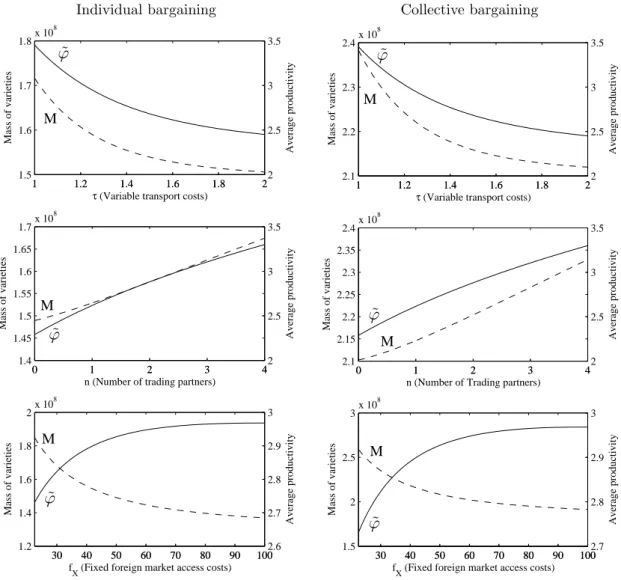
5 Unemployment and Trade Liberalization

This section discusses three globalization scenarios: (i) a reduction of variable trade costs, (ii) an increase in the number of trade relations and (iii) a drop in the fixed foreign distribution costs fX. The first and the third scenario capture technological (transportation costs) and political (tariffs, technical barriers to trade) change, while the second addresses the emergence of new countries into the global trading system. We describe the interaction of trade liberalization and unemployment in two steps. First, we consider the case where trade affects aggregate outcomes through the selection effect only (ν= 0). This isolates the novel mechanism introduced by Melitz (2003) and characterizes a particularly tractable special case. Then we analyze the more intricate case where trade also affects outcomes through an external scale effect, as in Krugman (1980) and in much of the subsequent literature.

5.1 The equilibrium rate of unemployment

The steady-state rate of unemployment is linked to the degree of labor market tightness θ and the importance of labor market churning, as captured by s, via the standard Beveridge curve

u(θ) = s

s+θm(θ). (20)

This condition ensures that the flows in and out of the unemployment pool are equal. As in standard search-matching models, the rate of unemployment is a decreasing function of the vacancy-unemployment ratio. Since we have shown in Propositions 1 and 2 that θis increasing in the level of aggregate productivity, it is sufficient to know how trade affects Φ≡M^σ−1ν ϕ˜ in order to characterize its impact on employment.

As usual, the equilibrium mass of firms is such that the labor market clears. Given that all workers are employed by domestic firms

M_D[l_D( ˜ϕ_D) +n%l_X( ˜ϕ_X)] = [1−u(θ)]L , (21)

whereLis the size of the labor force andM_D is the mass of domestic producers in each country.

Due to imports from foreign firms, input diversityM (i.e., the number of available varieties) is higher and equal toM =M_D(1 +n%).

Lemma 2 Equilibrium input diversity is determined by the Labor Market Clearing (LMC) con- dition which is a function of labor market tightness θand average productivity ϕ. For individual˜ bargaining, the LMC reads

LM CI:MI(θI) =



(1 +n%) (1−u(θI))L

1−β σ−β

1−δ r+s





˜ ϕ r+δ

1+r

FE

1−G(ϕ^∗_D)+fD +n%fX









σ−1 σ−1−ν

. (22)

For collective bargaining, the LMC is given by

LM C_C :M_C(θ_C) =



(1 +n%) (1−u(θ_C))L

1−β σ

1−δ r+s





˜ ϕ r+δ

1+r

FE

1−G(ϕ^∗_D)+f_D+n%f_X









σ−1 σ−1−ν

.

(23) Surprisingly enough, the sign of the relationship between input diversity M and aggregate employment is not always positive. This is because M has two opposite effects: (i) at the aggregate level, a larger number of firms naturally increases the number of employees; (ii) at the firm level, economies of scale implies that more input diversity raises revenues per worker so that firms have to be smaller for the ZCP condition to be satisfied.

When ν = 0, the scale effect is ruled out and so M is always increasing in the level of employment, as one might expect. On the other hand, whenσ < ν+1,so that firms enjoy strong market power and economies of scale are significant,M is decreasing in aggregate employment because the effect at the firm level dominates. Given that empirical studies typically yield estimates forσ above 2 and forν in the interval (0,1), we restrict our attention to cases where σ > ν+ 1.²⁴ In this case, the LMCs define upward-sloping loci because employment is increasing inθ so that labor market clearing requires the mass of producer to be larger.

24Egger and Kreickemeier (2007) also impose a similar restriction in order to ensure that their equilibrium is stable. Note that the conditionσ < ν+ 1 implies that the elasticity of aggregate productivity Φ with respect to input diversityM is smaller than unity.

5.2 Trade and unemployment without external economies of scale

In the absence of external economies of scale, i.e. whenν = 0, average and aggregate productiv- ity coincide since input diversity drops out from the description of the labor market equilibrium.

It is therefore sufficient to see how average productivity, ˜ϕ, changes in our globalization sce- narios. Trade affects the distribution of productivities across intermediate input producers by reallocating labor towards exporters and away from purely domestic firms, both at the exten- sive and at the intensive margin. The effect of trade liberalization on average productivity is nevertheless ambiguous because ˜ϕ factors in the output loss in export transit.

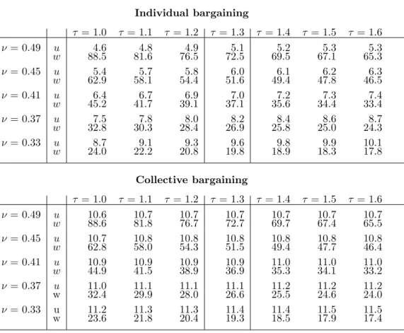
Part (i) of the following proposition gives a sufficient condition under which some liberaliza- tion scenarios always lead to an increase in aggregate employment. Part (ii) derives necessary and sufficient conditions for the case where the productivity distribution G(ϕ) belongs to the Pareto family of distributions, as usually done in the literature on heterogeneous firms.²⁵ Proposition 3 Assume that there are no economies of scale (ν = 0) and that the conditions stated in Propositions 1 and 2 are met.

(i) If f_X ≥ f_D, a reduction of variable trade costs τ or an increase in the number of trading partners n lead to a fall in the equilibrium rate of unemployment and a rise in the real wage, regardless of whether wages are bargained individually or collectively. A fall in fixed foreign distribution costs has an ambiguous effect on labor market outcomes.

(ii) Let firms draw their productivities from a Pareto distribution with dispersion parameter γ such that γ > σ−1. Then, regardless of the wage bargaining regime, the equilibrium rate of unemployment falls and the real wage rises

(a) due to a reduction in τ or an increase in n if and only if ^σ−1_γ

1 +nτ^−γ(f_D/f_X)^σ−1γ

≥

f_D fX −1,

(b) and due to a reduction in f_X if and only if _(σ−1)^γ2 2 ≥ _f ^fX

X−f_D

1 +nτ^−γ

fD

fX

_σ−1^γ .

The new insight in Melitz (2003) is that trade liberalization reallocates market shares towards efficient firms. Exporters, however, also incur iceberg transport costs which have to be deducted from the productivity gains at the factory gate. Whether or not trade liberalization enhances average productivity depends on which of these two adjustments prevails.²⁶ When f_X > f_D,

25See Egger and Kreickemeier, 2007; Bernard, Redding, Schott, 2007; Helpman, Melitz, Yeaple, 2004.

26Melitz (2003) briefly alludes to the ambiguity of the relationship between trade liberalization and ˜ϕ (see footnote 26, page 1713). He also introduces a measure of productivity at the factory gate and shows that it is always lower in autarky.

revenues generated on each foreign market have to exceed domestic revenues. In other words, the higher efficiency of exporting firms offsets both transport costs and the difference between f_X and f_D. This is why the selection effect always dominates the losses in export transit. On the other hand, whenfX < fD, some of the transport costs are compensated by lower fixed costs in foreign markets. Then the productivity gains at the factory gate due to trade liberalization are not necessarily higher than the increase in export losses.

A reduction in fixed costs of exportf_X triggers similar adjustments than a decrease inτ: it raises the domestic thresholdϕ^∗_D and lowers the export thresholdϕ^∗_X. Yet, it reallocates market shares in a different way. Whereas a decrease inτ raises the combined market shares of firms that already exported prior to liberalization, a decrease infX only benefits new exporters which are, on average, less productive than existing ones. Hence, the overall effect on average productivity is ambiguous and depends on whether the new exporters are on average more productive than the economy-wide average before the fall in fX.

The region where the relationship between trade openness and average productivity is neg- ative depends on the other parameters of the model. It can be characterized when parametric assumptions are imposed on the sampling distributionG(ϕ), as shown in part (ii) of Proposition 3 for cases where the sampling distribution is Pareto. Note that the effect of f_X is non-linear, since the stated parameter restrictions depends on f_X −f_D. If that difference is negative, a reduction in fixed market access costs always lowers unemployment.

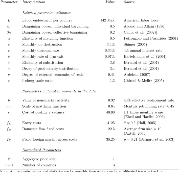
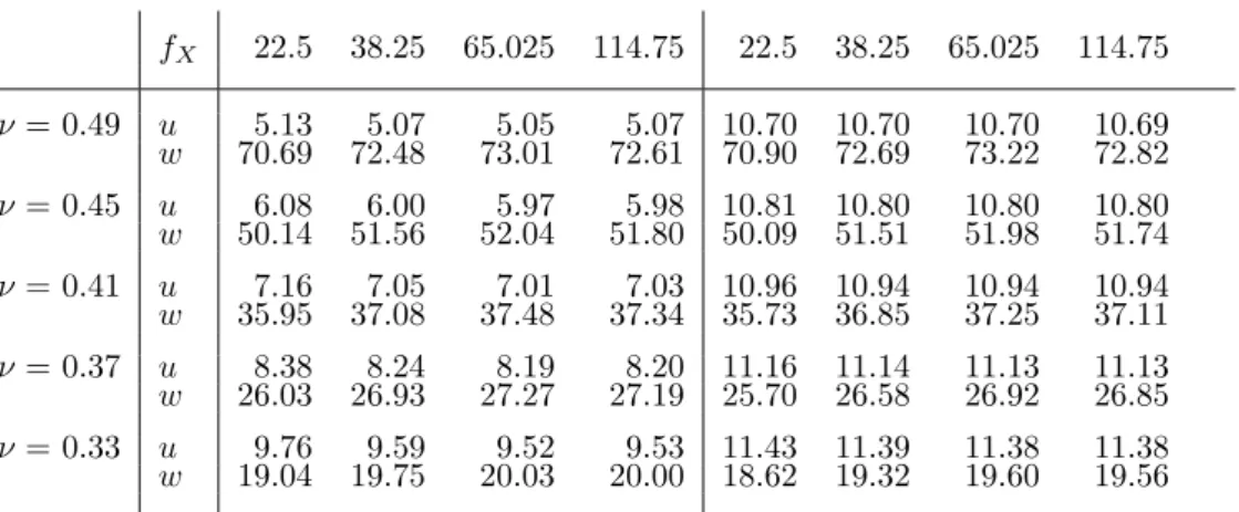
In section 6 we calibrate the model towards U.S. data. This allows to assess whether the conditions required for a beneficial impact of trade liberalization on labor market outcomes are likely to be met in reality or not. The calibration will also highlight the differences across bargaining regimes.²⁷

5.3 Equilibrium with external economies of scale

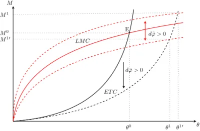
Labor market tightness, real wages and input diversity are determined jointly when there are external economies of scale (ν > 0). Their equilibrium values follow from the Job Creation, Wage Curve and Labor Market Clearing conditions, as defined in Sections 3and 5.1. To clarify

27It is easy to show that – everything else equal – unemployment reacts more strongly to aggregate productivity in the case of individual bargaining than in the case of collective bargaining when b = 0. When b > 0, the comparison is ambiguous. Since theceteris paribusassumption across the two scenarios is problematic (βmeasures different effective bargaining power in each case), we compare scenarios in the quantitative exercise of section6.

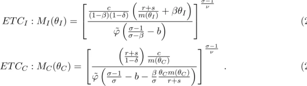
the analysis, we combine the Job Creation and Wage Curve into one equation that we label Equilibrium Tightness Condition (ETC). As the LMC, the ETC defines a mapping between input diversity M and labor market tightnessθ. We can then combine the LMC and the ETC for each bargaining environment to pin down the equilibrium values ofM and θ.Using (9) and (10) for individual, (12) and (11) for collective bargaining, we obtain

ET CI :MI(θI) =





c (1−β)(1−δ)

r+s

m(θI) +βθI

˜ ϕ

σ−1 σ−β −b





σ−1 ν

(24)

ET C_C :M_C(θ_C) =





r+s 1−δ

c m(θC)

˜ ϕ

σ−1

σ −b− ^β_σ^θCm(θ_r+s^C)





σ−1 ν

. (25)

The ETCs are upward-sloping in each bargaining regime because more input diversity raises efficiency and thus compensates the increase in recruitment costs as θ goes up. Given that the LMCs conditions are also increasing, equilibrium existence and uniqueness are not anymore ensured but can be established imposing empirically reasonable restrictions.²⁸

Lemma 3 Whenν≥0,equilibrium tightness and input diversity are pinned down by the system {(22),(24)} for the case of individual bargaining and by {(23),(25)} for the case of collective bargaining. Assume that the aggregate matching function is Cobb-Douglas, so that m(θ) = m0θ^−α, with m0 >0 and α∈(0,1). In case of individual bargaining, a sufficient condition for equilibrium existence and uniqueness is ν/(σ−1)< α. For the collective bargaining scenario, a sufficient condition is ν/(σ−1)< min [α,¹₂].

Figure3 shows the equilibrium conditions for the case of individual bargaining when wages are bargained at the individual level. Under the parameter restrictions presented in Lemma 3, both the ETC and the LMC start in the origin. The ETC is strictly convex while the LMC is strictly concave over the relevant parameter ranges. The LMC converges to some upper bound on input diversity ¯M while the ETC diverges. The collective bargaining case looks almost identical.²⁹ Hence, the existence of a unique equilibrium (point E) is guaranteed. As ν → 0,

28As explained in subsection5.1, whenσ < ν+ 1, the LMCs conditions are decreasing inθ. Hence, there always exists a unique equilibrium when this parameter restriction is satisfied. Yet, we do not focus on this case because it is neither theoretically realistic nor empirically relevant.

29 The only difference is that theET CClocus asymptotes towards some tightness ¯θ >0 implicitly determined by ^β_σ^θm¯ (^θ¯)

r+s =^σ−1_σ −b >0.