Essays on the Liquidity Trap, Oil Shocks, and the Great Moderation

(1)

Essays on the Liquidity Trap, Oil

Shocks, and the Great Moderation

A thesis presented

by

Anton Nakov

to

the Department of Economics and Business

in partial ful llment of the requirements

for the degree of

Doctor of Philosophy

in

Economics

Universitat Pompeu Fabra

Barcelona

November 2007

(2)

Dipòsit legal: B.9515-2008

(3)

Universitat Pompeu Fabra

Department of Economics and Business

The undersigned hereby certify that they have read and recommend to the Faculty

of Graduate Studies for acceptance a thesis entitled “Essays on the Liquidity Trap,

Oil Shocks, and the Great Moderation” by Anton Nakov in partial ful llment of the

requirements for the degree of Doctor of Philosophy.

Date: November 2007

Supervisor: ________________________________________

Prof. Jordi Galí

Readers: ________________________________________

________________________________________

(4)

Universitat Pompeu Fabra

Department of Economics and Business

Author: Anton Nakov

Contact: Tellez 12 B Entreplanta “I”; 28007 Madrid; Spain

Title: Essays on the Liquidity Trap, Oil Shocks, and the Great Moderation

Degree: Doctor of Philosophy

Date: November 2007

Permission is herewith granted to Universitat Pompeu Fabra to circulate and to

have copied for non-commercial purposes, at its discretion, the above title upon the

request of individuals or institutions.

Signature of Author: ________________________________________

The author reserves other publication rights, and neither the thesis nor extensive

extracts from it may be printed or otherwise reproduced without the author's written

permission.

The author attests that permission has been obtained for the use of any

copy-righted material appearing in this thesis (other than brief excerpts requiring only proper

acknowledgement in scholarly writing) and that all such use is clearly acknowledged.

(5)

To my family

(6)

Acknowledgments

More than anyone I would like to thank Prof. Jordi Galí for the invaluable

guidance and inspiration that having him as a thesis advisor has meant to me.

Without him this work would not have been possible.

I am indebted also to many people from the Barcelona economics

com-munity who, together with the graduate program at Universitat Pompeu Fabra,

turned me from someone who was hardly aware about many of the issues into

somebody who aspires to contribute to economic research at the highest level.

In particular, I have bene ted immensely from interaction with Albert Marcet,

Ramon Marimon, Fabio Canova, Michael Reiter, Kosuke Aoki, and Jaume

Ven-tura. Needless to say, I have learned a great deal from my co-authors Max

Gillman and Andrea Pescatori, as well as from fellow students Krisztina

Mol-nar, Lutz Weinke, Philip Saure, Gustavo Solorzano, Helmuts Azacis and Peter

Vida. To all these people I am very, very grateful.

Part of the work on this thesis was undertaken while I was an intern at

the ECB and I would like to thank the people there for their hospitality,

es-pecially Massimo Rostagno and Victor Lopez Perez. I enjoyed and learned

much also during my internship at the IMF, for which I am grateful to Roberto

Garcia-Saltos, Douglas Laxton and Pau Rabanal. Finally, I would like to thank

my colleagues at Banco de España, especially Juan Francisco Jimeno and

Fer-nando Restoy for useful comments and support during the nal stage of my

dissertation. Last but not least, I am grateful for nancial support from Agencia

Española de Cooperacion Internacional (Becas MAE).

(7)

vi

Preface

. . .

1 1 Optimal and Simple Monetary Policy Rules with Zero Floor

on the Nominal Interest Rate

. . .

4

1.1 Introduction . . . 4

1.2 Model . . . 9

1.3 Optimal Discretionary Policy with Zero Floor. . . 14

1.4 Optimal Commitment Policy with Zero Floor . . . 19

1.5 Targeting Rules with Zero Floor . . . 24

1.6 Simple Instrument Rules with Zero Floor . . . 27

1.7 Welfare Ranking of Alternative Rules . . . 31

1.8 Sensitivity Analysis . . . 35

1.8.1 Parameters of the Natural Real Rate Process . . . 35

1.8.2 Instrument Rule Speci cation . . . 38

1.8.3 Endogenous In ation Persistence and the Zero Floor . . . 39

1.9 Conclusions . . . 41

1.A Numerical Algorithm . . . 43

1.B Figures . . . 47

(8)

Contents vii

2 In ation–Output Gap Trade-off with a Dominant Oil Supplier

. .

57

2.2 The Model . . . 60

2.2.1 Oil Importing Country . . . 62

2.2.2 Oil Exporting Countries. . . 64

2.2.3 Equilibrium Conditions for a Given Oil Supply . . . 69

2.2.4 The Dominant Oil Exporter's Problem . . . 74

2.2.5 Flexible Price Benchmarks . . . 75

2.2.6 Equilibrium with Sticky Prices . . . 82

2.2.7 Calibration . . . 84

2.3 Steady State and Comparative Statics . . . 86

2.4 Dynamic Properties of the Model . . . 87

2.4.1 US technology shock . . . 88

2.4.2 Oil technology shock . . . 90

2.4.3 Fringe capacity shock . . . 92

2.4.4 Monetary policy shock . . . 93

2.4.5 Summary and policy implications . . . 94

2.4.6 A note on Taylor-type reaction to the oil price . . . 96

2.4.7 Variance decomposition . . . 97

2.5 Sensitivity Analysis . . . 99

2.5.1 The elasticity of oil in production. . . 99

2.5.2 Monetary policy . . . 100

2.6 Conclusion . . . 104

2.A First Order Conditions of OPEC's Problem . . . 106

2.B GDP Gap Derivation and Proof of Proposition 3 . . . 107

(9)

Contents viii

3 Oil and the Great Moderation

. . . .

123

3.2 Related Literature . . . 125

3.3 Volatility Reduction Facts. . . 128

3.4 The Log-Linearized Model . . . 129

3.4.1 Dynamic IS curve . . . 130

3.4.2 Phillips curve . . . 131

3.4.3 Monetary policy . . . 132

3.4.4 Oil sector . . . 132

3.4.5 What factors could cause moderation? . . . 133

3.5 Data and Methodology . . . 135

3.6 Priors and Estimation Results . . . 138

3.6.1 Choice of priors . . . 138

3.6.2 Estimation results . . . 139

3.7 Implications. . . 141

3.7.1 What accounts for the Moderation? . . . 141

3.7.2 Changes in the Phillips curve . . . 144

3.7.3 Changes in the relative importance of shocks . . . 145

3.8 Comparison of the Results with the Literature. . . 147

3.9 Conclusions . . . 149

3.A Calibrated parameters . . . 150

3.B Figures . . . 150

(10)

Preface

The thesis studies three distinct issues in monetary economics using a common

dynamic general equilibrium approach under the assumptions of rational expectations

and nominal price rigidity.

The rst chapter deals with the so-called “liquidity trap” – an issue which was

raised originally by Keynes in the aftermath of the Great Depression. Since the

nomi-nal interest rate cannot fall below zero, this limits the scope for expansionary monetary

policy when the interest rate is near its lower bound. The chapter studies the conduct

of monetary policy in such an environment in isolation from other possible

stabiliza-tion tools (such as scal or exchange rate policy). In particular, a standard New

Key-nesian model economy with Calvo staggered price setting is simulated under various

alternative monetary policy regimes, including optimal policy. The challenge lies in

solving the (otherwise linear) stochastic sticky price model with an explicit

occasion-ally binding non-negativity constraint on the nominal interest rate. This is achieved by

parametrizing expectations and applying a global solution method known as

“colloca-tion”. The results indicate that the dynamics and sometimes the unconditional means of

the nominal rate, in ation and the output gap are strongly affected by uncertainty in the

presence of the zero lower bound. Commitment to the optimal rule reduces

uncondi-tional welfare losses to around one-tenth of those achievable under discretionary policy,

while constant price level targeting delivers losses which are only 60% larger than

un-der the optimal rule. On the other hand, conditional on a strong de ationary shock,

simple instrument rules perform substantially worse than the optimal policy even if the

(11)

Preface 2

unconditional welfare loss from following such rules is not much affected by the zero

lower bound per se.

The second thesis chapter (co-authored with Andrea Pescatori) studies the

impli-cations of imperfect competition in the oil market, and in particular the existence of a

welfare-relevant trade-off between in ation and output gap volatility. In the standard

New Keynesian model exogenous oil shocks do not generate any such tradeoff: under

a strict in ation targeting policy, the output decline is exactly equal to the ef cient

out-put contraction in response to the shock. I propose an extension of the standard model

in which the existence of a dominant oil supplier (such as OPEC) leads to inef cient

uctuations in the oil price markup, re ecting a dynamic distortion of the economy's

production process. As a result, in the face of oil sector shocks, stabilizing in ation does

not automatically stabilize the distance of output from rst-best, and monetary

policy-makers face a tradeoff between the two goals. The model is also a step away from

discussing the effects of exogenous oil price changes and towards analyzing the

impli-cations of the underlying shocks that cause the oil price to change in the rst place. This

is an advantage over the existing literature, which treats the macroeconomic effects and

policy implications of oil price movements as if they were independent of the

underly-ing source of disturbance. In contrast, the analysis in this chapter shows that conditional

on the source of the shock, a central bank confronted with the same oil price change

may nd it desirable to either raise or lower the interest rate in order to improve welfare.

The third thesis chapter (co-authored with Andrea Pescatori) studies the extent to

which the rise in US macroeconomic stability since the mid-1980s can be accounted

for by changes in oil shocks and the oil share in GDP. This is done by estimating with

(12)

Preface 3

and after 1984 - and conducting counterfactual simulations. In doing so we nest two

other popular explanations for the so-called “Great Moderation”: (1) smaller (non-oil)

shocks; and (2) better monetary policy. We nd that the reduced oil share can account

for around one third of the in ation moderation, and about 13% of the GDP growth

moderation. At the same time smaller oil shocks can explain approximately 7% of

GDP growth moderation and 11% of the in ation moderation. Thus, the oil share and

oil shocks have played a non-trivial role in the moderation, especially of in ation, even

if the bulk of the volatility reduction of output growth and in ation is attributed to

(13)

Chapter 1 Optimal and Simple Monetary Policy Rules

with Zero Floor on the Nominal Interest

Rate

1.1 Introduction

An economy is said to be in a “liquidity trap” when the monetary authority cannot

achieve a lower nominal interest rate in order to stimulate output. Such a situation

can arise when the nominal interest rate has reached its zero lower bound (ZLB),

be-low which nobody would be willing to lend, if money can be stored at no cost for a

nominally riskless zero rate of return.

The possibility of a liquidity trap was rst suggested by Keynes (1936) with

ref-erence to the Great Depression of the 1930s. At that time he compared the effectiveness

of monetary policy in such a situation with trying to “push on a string”. After WWII

and especially during the high in ation period of the 1970s interest in the topic receded,

and the liquidity trap was relegated to a hypothetical textbook example. As Krugman

(1998) noticed, of the few modern papers that dealt with it most concluded that “the

liquidity trap can't happen, it didn't happen, and it won't happen again”.

With the bene t of hindsight, however, it did happen, and to no less than Japan.

Figure 1.1 illustrates this, showing the evolution of output, in ation, and the short-term

nominal interest rate following the collapse of the Japanese real estate bubble of the

late 1980s. The gure exhibits a persistent downward trend in all three variables, and in

(14)

1.1 Introduction 5

particular the emergence of de ation since 1998 coupled with a zero nominal interest

rate since 1999.

Motivated by the recent experience of Japan, the aim of the present study is to

contribute a quantitative analysis of the ZLB issue in a standard sticky price model

under alternative monetary policy regimes. One the one hand, the paper characterizes

optimal monetary policy in the case of discretion and commitment.1 _{And on the other}

hand, it studies the performance of several simple monetary policy rules, modi ed to

comply with the zero oor, relative to the optimal policy. The analysis is carried out

within a stochastic general equilibrium model with monopolistic competition and Calvo

(1983) staggered price setting, under a standard calibration to the postwar US economy.

The main ndings are as follows: the optimal discretionary policy with zero oor

involves a de ationary bias, which may be signi cant for certain parameter values and

which implies that any quantitative analyses of discretionary biases of monetary policy

that ignore the zero lower bound may be misleading. In addition, optimal discretionary

policy implies much more aggressive cutting of the interest rate when the risk of

de-ation is high, compared to the corresponding policy without zero oor. Such a policy

helps mitigate the depressing effect of private sector expectations on current output and

prices when the probability of falling into a liquidity trap is high.2

In contrast, optimal commitment policy involves less preemptive lowering of the

interest rate in anticipation of a liquidity trap, but it entails a promise for sustained

mon-1 _{The part of the paper on optimal policy is similar to independent work by Adam and Billi (2006) and}

Adam and Billi (2007). The added value is to quantify and compare the performance of optimal policy to that of a number of suboptimal rules (including discretionary policy) in the same stochastic sticky price setup.

2 _{An early version of this paper comparing the performance of optimal discretionary policy with three}

(15)

1.1 Introduction 6

etary policy easing following an exit from a trap. This type of commitment enables the

central bank to achieve higher expected in ation and lower real rates in periods when

the zero oor on nominal rates is binding.3 _{As a result, under the baseline calibration,}

the expected welfare loss under commitment is only around one-tenth of the loss

un-der optimal discretionary policy. This implies that the cost of discretion may be much

higher than normally considered when abstracting from the zero lower bound issue.

The average welfare losses under simple instrument rules are 8 to 20 times bigger

than under the optimal rule. However, the bulk of these losses stem from the intrinsic

suboptimality of simple instrument rules, and not from the zero oor per se. This is

related to the fact that under these rules the zero oor is hit very rarely - less than 1%

of the time - compared to optimal policy, which visits the liquidity trap one-third of

the time. On the other hand, conditional on a large de ationary shock, the relative

performance of simple instrument rules deteriorates substantially vis-a-vis the optimal

policy.

Issues of de ation and the liquidity trap have received considerable attention

re-cently, especially after the experience of Japan.4 _{In an in uential article Krugman}

(1998) argued that the liquidity trap boils down to a credibility problem in which private

agents expect any monetary expansion to be reverted once the economy has recovered.

As a solution he suggested that the central bank should commit to a policy of high future

in ation over an extended horizon.

3 _{This basic intuition was suggested already by Krugman (1998) based on a simpler model.}

4 _{A partial list of relevant studies includes Krugman (1998), Wolman (1998), McCallum (2000),}

(16)

1.1 Introduction 7

More recently, Jung et al. (2005) have explored the effect of the zero lower bound

in a standard sticky price model with Calvo price setting under the assumption of perfect

foresight. Consistent with Krugman (1998), they conclude that optimal commitment

policy entails a promise of a zero nominal interest for some time after the economy

has recovered. Eggertsson and Woodford (2003) study optimal policy with zero lower

bound in a similar model in which the natural rate of interest is allowed to take two

different values. In particular, it is assumed to become negative initially and then to

jump to its “normal” positive level with a xed probability in each period. These authors

also conclude that the central bank should create in ationary expectations for the future.

Importantly, they derive a moving price level targeting rule that delivers the optimal

policy in this model.

One shortcoming of much of the modern literature on monetary policy rules is

that it largely ignores the ZLB issue or at best uses rough approximations to address

the problem. For instance Rotemberg and Woodford (1997) introduce nominal rate

targeting as an additional central bank objective, which ensures that the resulting path

of the nominal rate does not violate the zero lower bound too often. In a similar vein,

Schmitt-Grohe and Uribe (2004) exclude from their analysis instrument rules that result

in a nominal rate the average of which is less than twice its standard deviation. In both

cases therefore one might argue that for suf ciently large shocks that happen with a

probability as high as 5%, the derived monetary policy rules are inconsistent with the

zero lower bound.

On the other hand, of the few papers that do introduce an explicit non-negativity

constraint on nominal interest rates, most simplify the stochastics of the model, for

(17)

1.1 Introduction 8

(Eggertsson and Woodford (2003); Wolman (1998)). Even then, the zero lower bound

is effectively imposed as an initial (“low”) condition and not as an occasionally binding

constraint.5 _{While this assumption may provide a reasonable rst-pass at a}

quantita-tive analysis, it may be misleading to the extent that it ignores the occasionally binding

nature of the zero interest rate oor.

Other studies (e.g. Coenen et al. (2004)) lay out a stochastic model but

know-ingly apply inappropriate solution techniques which rely on the assumption of certainty

equivalence. It is well known that this assumption is violated in the presence of a

non-linear constraint such as the zero oor but nevertheless these researchers have imposed

it for reasons of tractability (admittedly they work with a larger model than the one

studied here). Yet forcing certainty equivalence in this case amounts to assuming that

agents ignore the risk of the economy falling into a liquidity trap when making their

optimal decisions.

The present study contributes to the above literature by solving numerically a

stochastic general equilibrium model with monopolistic competition and sticky prices

with an explicit occasionally binding zero lower bound, using an appropriate global

solution technique that does not rely on certainty equivalence. It extends the analysis

of Jung et al. (2005) to the stochastic case with an AR(1) process for the natural rate of

interest.

After a brief outline of the basic framework adopted in the analysis (section 1.2),

the paper characterizes and contrasts the optimal discretionary and optimal commitment

policies (sections 1.3 and 1.4). It then analyzes the performance of a range of simple

5 _{Namely, the zero oor binds for the rst several periods but once the economy transits to the “high”}

(18)

1.2 Model 9

instrument and targeting rules (sections 1.5 and 1.6) consistent with the zero oor.6

Sec-tions 1.4 to 1.6 include a comparison of the conditional performance of all rules in a

simulated liquidity trap, while section 1.7 presents their average performance, including

a ranking according to unconditional expected welfare. Section 1.8 studies the

sensi-tivity of the ndings to various parameters of the model, as well as the implications of

endogenous in ation persistence for the ZLB issue and the last section concludes.

1.2 Model

While in principle the zero lower bound phenomenon can be studied in a model with

exible prices, it is with sticky prices that the liquidity trap becomes a real problem.

The basic framework adopted in this study is a stochastic general equilibrium model

with monopolistic competition and staggered price settinga laCalvo (1983) as in Galí

(2003) and Woodford (2003). In its simplest log-linearized7 _{version the model consists}

of three building blocks, describing the behavior of households, rms and the monetary

authority.

The rst block, known as the “IS curve”, summarizes the household's optimal

consumption decision,

xt=Etxt+1 (it Et t+1 rnt): (1.1)

6 _{These rules include truncated Taylor-type rules reacting to contemporaneous, expected future, or past,}

in ation, output gap, or price level; with or without “interest rate smoothing”; truncated rst-difference rules; price level targeting; and strict in ation targeting rules.

7 _{It is important to note that, like in the studies cited in the introduction, the objective here is a modest}

(19)

1.2 Model 10

It relates the “output gap”xt(i.e. the deviation of output from its exible price

equilib-rium) positively to the expected future output gap and negatively to the gap between the

ex-ante real interest rate,it Et t+1;and the “natural” (i.e. exible price equilibrium)

real rate, rn

t (which is known to all agents at time t). Consumption smoothing

ac-counts for the positive dependence of current on expected future output demand, while

intertemporal substitution implies the negative effect of the ex-ante real interest rate.

The interest rate elasticity of output, , corresponds to the elasticity of intertemporal

subsitution of the consumers' utility function.

The second building block of the model is a “Phillips curve”-type equation, which

derives from the optimal price setting decision of monopolistically competitive rms

under the assumption of staggered price settinga laCalvo (1983),

t = Et t+1+ xt; (1.2)

where is the time discount factor and , “the slope” of the Phillips curve, is related

inversely to the degree of price stickiness8_{. Since rms are unable to adjust prices}

optimally every period, whenever they have the opportunity to do so, they choose to

price goods as a markup over a weighted average of current and expected future

mar-ginal costs. Under appropriate assumptions on technology and preferences, marmar-ginal

costs are proportional to the output gap, resulting in the above Phillips curve. Here this

relation is assumed to hold exactly, ignoring the so-called “cost-push” shock, which

sometimes is appendedad-hocto generate a short-term trade-off between in ation and

output gap stabilization.

8 _{In the underlying sticky price model the slope} _{is given by}_{[ (1 +}_'"_)] 1

(1 ) (1 )( 1₊

');where is the fraction of rms that keep prices unchanged in each period, 'is the (inverse) wage

(20)

1.2 Model 11

The nal building block models the behavior of the monetary authority. The

model assumes a “cashless limit” economy in which the instrument controlled by the

central bank is the nominal interest rate. One possibility is to assume a benevolent

monetary policy maker seeking to maximize the welfare of households. In that case, as

shown in Woodford (2003), the problem can be cast in terms of a central bank that aims

to minimize (under discretion or commitment) the expected discounted sum of losses

from output gaps and in ation, subject to the optimal behavior of households (1.1) and

rms (1.2), and in addition, the zero nominal interest rate oor:

Min

it; t;xt

E0

1

X

t=0

t 2

t + x2t (1.3)

s.t. (1:1); (1:2)

it 0 (1.4)

where is the relative weight of the output gap in the central bank's loss function.

An alternative way of modeling monetary policy is to assume that the central bank

follows some sort of simple decision rule that relates the policy instrument, implicitly

or explicitly, to other variables of the model. An example of such a rule, consistent with

the zero oor, is a truncated Taylor rule,

it= max [0; r + + ( t ) + xxt] (1.5)

wherer is an equilibrium real rate, is an in ation target, and and _xare response

coef cients for in ation and the output gap.

To close the model one needs to specify the behavior of the natural real rate. In the

fuller model the latter is a composite of a variety of real disturbances, including shocks

(21)

1.2 Model 12

I assume that the natural real rate follows an exogenous mean-reverting process,

b

r_tn= _brn_t ₁+ t; (1.6)

wherer_bn

t rtn r , is the deviation of the natural real rate from its unconditional mean,

r ; tare i.i.d. N(0; 2)real shocks, and0 <1is a persistence parameter.

The equilibrium conditions of the model therefore include the constraints (1.1),

(1.2), and either a set of rst-order optimality conditions (in the case of optimal policy),

or a simple rule like (1.5). In either case the resulting system of equations cannot be

solved with standard solution methods relying on local approximation because of the

non-negativity constraint on the nominal rate. Hence I solve them with a global solution

technique known as “collocation”. The rational expectations equilibrium with

occasion-ally binding constraint is solved by way of parametrizing expectations (Christiano and

Fischer 2000), and is implemented with the MATLAB routines developed by Miranda

and Fackler (2001). Appendix 1.A outlines the simulation algorithm, while the

follow-ing sections report the results.

1.2.1 Baseline Calibration

The model's parameters are chosen to be consistent with the “standard” Woodford

(2003) calibration to the US economy, which is based on Rotemberg and Woodford

(1997) (Table 1.1). Thus, the slope of the Phillips curve (0.024), the weight of the

output gap in the central bank loss function (0.003), the time discount factor (0.993),

the mean (3% pa) and standard deviation (3.72%) of the natural real rate are all taken

directly from Woodford (2003). The persistence (0.65) of the natural real rate is

(22)

1.2 Model 13

Structural parameters

Discount factor 0.993 Real interest rate elasticity of output 0.25 Slope of the Phillips curve 0.024 Weight of the output gap in loss function 0.003 Natural real rate parameters

Mean (% per annum) r 3%

Standard deviation (annual) (rn₎ _3.72%

Persistence (quarterly) 0.65 Simple instrument rule coef cients

In ation target (% per annum) 0% Coef cient on in ation 1.5 Coef cient on output gap x 0.5

Interest rate smoothing coef cient i 0

Table 1.1. Baseline calibration (quarterly unless otherwise stated)

Adam and Billi (2006) (0.8) using more recent data.9 _{The real interest rate elasticity}

of aggregate demand (0.25)10 _{is lower than the elasticity assumed by Eggertsson and}

Woodford (2003) (0.5), but as these authors point out, if anything, a lower degree of

interest sensitivity of aggregate expenditure biases the results towards a more modest

output contraction as a result of a binding zero oor.11 _{In the simulations with simple}

rules, the baseline target in ation rate (0%) is consistent with the implicit zero target for

in ation in the central bank's loss function. The baseline reaction coef cients on in

a-tion (1.5), the output gap (0.5), and the lagged nominal interest rate (0) are standard in

the literature on Taylor (1993)-type rules. Section 8 studies the sensitivity of the results

to various parameter changes.

9 _{These parameters for the shock process imply that the natural real interest rate is negative about 15%}

of the time on an annual basis. This is slightly more often than with the standard Woodford calibration (10%).

10 _{This corresponds to a constant relative risk aversion of 4 in the underlying model.}

11 _{With the Woodford (2003) value of this parameter (6.25), the model predicts unrealistically large}

(23)

1.3 Optimal Discretionary Policy with Zero Floor 14

1.3 Optimal Discretionary Policy with Zero Floor

Abstracting from the zero oor, the solution to the discretionary optimization problem

is well known (Clarida, Gali and Gertler 1999)12_{. Under full discretion, the central}

bank cannot manipulate the beliefs of the private sector and it takes expectations as

given. The private sector is aware that the central bank is free to re-optimize its plan

in each period and, therefore, in a rational expectations equilibrium, the central bank

should have no incentives to change its plans in an unexpected way. In the baseline

model with no endogenous state variables, the discretionary policy problem reduces to

a sequence of static optimization problems in which the central bank minimizes current

period losses by choosing the current in ation, output gap, and nominal interest rate as

a function only of the exogenous natural real rate,rn_t.

The solution without zero bound then is straightforward: in ation and the output

gap are fully stabilized at their (zero) targets in every period and state of the world,

while the nominal interest rate moves one-for-one with the natural real rate. This is

depicted by the dashed lines in Figure 1.2. With this policy the central bank is able to

achieve the globally minimal welfare loss of zero at all times.

With the zero oor, the basic problem of discretionary optimization (without

en-dogenous state variables) can still be cast as a sequence of static problems. The

La-grangian can be written as,

Lt=

1 2

2

t + x

2

t + 1t[xt f1t+ (it f2t)] + 2t[ t xt f2t] + 3tit (1.7)

where ₁_t is the Lagrange multiplier associated with the IS curve (1.1), ₂_t with the

Phillips curve (1.2), and ₃_twith the zero constraint (1.4). The functionsf1t=Et(xt+1),

(24)

and f2t = Et( t+1) are private sector expectations which the central bank takes as

given. Noticing that ₃_t= ₁_t;the Kuhn-Tucker conditions for this problem can be

written as:

t+ 2t = 0 (1.8)

xt+ 1t 2t = 0 (1.9)

it 1t = 0 (1.10)

it 0 (1.11)

1t 0 (1.12)

Substituting (1.8) and (1.9) into (1.10), and combining the result with (1.1), (1.2), and

(1.4), a Markov perfect rational expectations equilibrium should satisfy:

xt Etxt+1+ (it Et t+1 rtn) = 0 (1.13)

t xt Et t+1 = 0 (1.14)

it( xt+ t) = 0 (1.15)

it 0 (1.16)

xt+ t 0 (1.17)

Notice that (1.15) implies that the typical “targeting rule” involving in ation and

the output gap is satis ed whenever the zero oor on the nominal interest rate is not

binding,

xt+ t = 0; (1.18)

(25)

However, when the zero oor is binding, from (1.13) the dynamics are governed

by

xt+ pt rnt = Etxt+1+ Etpt+1 (1.19)

if it = 0

wherept is the (log) price level. Note that it is no longer possible to set in ation and

the output gap to zero at all times, for such a policy would require a negative nominal

interest rate when the natural real interest rate falls below zero. Moreover, (1.19) implies

that if the natural real rate falls so that the zero oor becomes binding, then since next

period's output gap and price level are independent of today's actions, for expectations

to be rational, the sum of the current output gap and price level must fall. The latter

is true for any process for the natural real interest rate which allows it to take negative

values.

An interesting special case, which replicates the ndings of Jung et al. (2005),

is the case of perfect foresight. By perfect foresight we mean that the natural real rate

jumps initially to some (possibly negative) value, after which it follows a deterministic

path (consistent with the expected path of an AR(1) process) back to its steady-state.

In this case the policy functions are represented by the solid lines in Figure 1.2. As

anticipated in the previous paragraph, at negative values of the natural real rate both the

output gap and in ation are below target. On the other hand, at positive levels of the

natural real rate, prices and output can be stabilized fully in the case of discretionary

optimization with perfect foresight. The reason for this is simple: once the natural real

rate is above zero, deterministic reversion to steady-state implies that it will never be

(26)

nominal rate (as in the case without zero oor), which is suf cient to fully stabilize

prices and output.

One of the contributions of this paper is to extend the analysis in Jung et al.

(2005) to the more general case in which the natural real rate follows a stochastic AR(1)

process. Figure 1.3 plots the optimal discretionary policies in the stochastic

environ-ment. Clearly optimal discretionary policy differs in several important ways both from

the optimal policy unconstrained by the zero oor and from the constrained

perfect-foresight solution. First of all, given the zero oor, it is in general no longer optimal to

set either in ation or the output gap to zero in any state of the world. In fact, in the

so-lution with zero oor, in ation falls short of target atanylevel of the natural real rate.

This gives rise to a “de ationary bias” of optimal discretionary policy, that is, an

aver-agerate of in ation below the target. Sensitivity analysis shows that for some plausible

parameter values the de ationary bias becomes quantitatively signi cant13_{. This}

im-plies that any quantitative analysis of discretionary biases in monetary models that does

not take into account the zero lower bound can be misleading.

Secondly, as in the case of perfect foresight, at negative levels of the natural real

rate, both in ation and the output gap fall short of their respective targets. However, the

deviations from target are larger in the stochastic case - up to 1.5 percentage points for

the output gap, and up to 15 basis points for in ation at a natural real rate of -3% under

the baseline calibration.

Third, above a positive threshold for the natural real rate, the optimal output gap

becomes positive, peaking around +0.5%.

(27)

Finally, at positive levels of the natural real rate the optimal nominal interest rate

policy with zero oor is bothmore expansionary(i.e. prescribing a lower nominal rate),

andmore aggressive(i.e. steeper) compared to the optimal policy without zero oor14_.

As a result, the nominal rate hits the zero oor at levels of the natural real rate as high

as 1.8% (and is constant at zero for lower levels of the natural real rate).

These results hinge on the combination of two factors: (1) the stochastic nature

of the natural real rate; and (2) the non-linearity induced by the zero oor. The effect

is an asymmetry in the ability of the central bank to respond to positive versus negative

shocks when the natural real rate is close to zero. Namely, while the central bank can

fully offset any positive shocks to the natural real rate because nothing prevents it from

raising the nominal rate by as much as is necessary, it cannot fully offset large enough

negative shocks. The most it can do in this case is to reduce the nominal rate down

to zero, which is still higher than the interest rate consistent with zero output gap and

in ation. Taking private sector expectations as given, the latter implies a higher than

desiredrealinterest rate, which depresses output and prices through the IS and Phillips

curves.

The above asymmetry is re ected in the private sector's expectations: a positive

shock in the following period is expected to be neutralized, while an equally probable

negative one is expected to take the economy into a liquidity trap. This gives rise to

a “de ationary bias” in the private sector's expectations, which in a forward-looking

economy has an impact on thecurrent evolution of output and prices. Absent an

en-dogenous state, the current evolution of the economy is all that matters for welfare, and

so it is optimal for the central bank to partially offset the depressing effect of

(28)

1.4 Optimal Commitment Policy with Zero Floor 19

tations on today's outcome by more aggressive lowering of the nominal rate when the

risk of de ation is high.

At suf ciently high levels of the natural real interest rate, the probability for the

zero oor to become binding tends to zero. Hence optimal discretionary policy

ap-proaches the unconstrained case, namely zero output gap and in ation, and a nominal

rate equal to the natural real rate. However, around the deterministic steady-state the

difference between the two policies - with and without zero oor - remains signi cant.

We have seen that in the baseline model with no endogenous states, optimal

dis-cretionary policy is independent of history. This means that it is only the current risk

of falling into a liquidity trap that matters for today's policy, regardless of whether the

economy is approaching a liquidity trap or has just recovered from one. This is in sharp

contrast with the optimal policy under commitment, which involves a particular type of

history dependence as the following section shows.

1.4 Optimal Commitment Policy with Zero Floor

In the absence of the zero lower bound the equilibrium outcome under optimal

discre-tion is globally optimal and therefore it is observadiscre-tionally equivalent to the outcome

under optimal commitment policy. The central bank manages to stabilize fully in ation

and the output gap while adjusting the nominal rate one-for-one with the natural real

rate.

However, this observational equivalence no longer holds in the presence of a zero

interest rate oor. While full stabilization under either regime is not possible, important

(29)

committing to deliver in ation in the future, the central bank can affect private sector's

expectations about in ation, and thus the real rate, even when the nominal interest rate

is constrained by the zero oor. This channel of monetary policy in simply unavailable

to a discretionary policy maker.

Using the Lagrange method as before, but this time taking into account the

depen-dence of expectations on policy choices, it is straightforward to obtain the equilibrium

conditions that govern the optimal commitment solution:

xt Etxt+1+ (it Et t+1 rtn) = 0 (1.20)

t xt Et t+1 = 0 (1.21)

t 1t 1 = + 2t 2t 1 = 0 (1.22)

xt+ 1t 1t 1= 2t = 0 (1.23)

it 1t = 0 (1.24)

it 0 (1.25)

1t 0 (1.26)

From conditions (1.22) and (1.23) it is clear that the Lagrange multipliers

inher-ited from the past period will have an effect on current policy. They in turn will depend

on the history of endogenous variables and in particular on whether the zero oor was

binding in the past. In this sense the Lagrange multipliers summarize the effect of

opti-mal commitment, which in contrast to optiopti-mal discretionary policy, involves a particular

type of history dependence.

Figures 1.4 to 1.6 plot the optimal policies in the case of commitment. The

g-ures illustrate speci cally the dependence of policy on ₁_t ₁;the Lagrange multiplier

(30)

rate is constrained by the zero oor ₁becomes positive, implying that the central bank

commits to a lower nominal rate, higher in ation and higher output gap in the following

period, conditional on the value of the natural real rate.

Since the commitment is assumed to be credible, it enables the central bank to

achieve higher expected in ation and a lower real rate in periods when the nominal

rate is constrained by the zero oor. The lower real rate reinforces expectations for

higher future output and thus further stimulates current output demand through the IS

curve. This, together with higher expected in ation stimulates current prices through

the expectational Phillips curve. Commitment therefore provides an additional channel

of monetary policy, which works through expectations and through the ex-ante real rate,

and which is unavailable to a discretionary monetary policy maker.

A standard way to illustrate the differences between optimal discretionary and

commitment policies is to compare the dynamic evolution of endogenous variables

un-der each regime in response to a single shock to the exogenous natural real rate. Figures

1.7 and 1.8 plot the impulse-responses for a small and a large negative shock to the

nat-ural real rate respectively. Notice that in the case of a small shock to the natnat-ural real

rate from its steady-state of 3% down to 2%, in ation and the output gap under optimal

commitment policy (lines with circles) remain almost fully stabilized. In contrast,

un-der discretionary optimization (lines with squares), in ation stays slightly below target

and the output gap remains about half a percentage point above target, consistent with

equation (1.18), as the economy converges back to its steady-state. The nominal

inter-est rate under discretion is about 1% lower than the one under commitment throughout

(31)

The picture changes substantially in the case of a large negative shock to the

nat-ural interest rate to -3%. Notably, under both commitment and discretion, the nominal

interest rate hits the zero lower bound, and remains there until two quarters after the

natural interest rate has returned to positive.15 _{Under discretionary optimization, both}

in ation and the output gap fall on impact, consistent with equation (1.19), after which

they converge towards their steady-state. The initial shortfall is signi cant, especially

for the output gap, amounting to about 1.5%. In contrast, under the optimal

commit-ment rule the initial output loss and de ation are much milder, owing to the ability of

the central bank to commit to a positive output gap and in ation once the natural real

rate has returned to positive.

An alternative way to compare optimal discretionary and commitment policies

in the stochastic environment is to juxtapose the dynamic paths that they prescribe for

endogenous variables under a particular path for the stochastic natural real rate16_{. The}

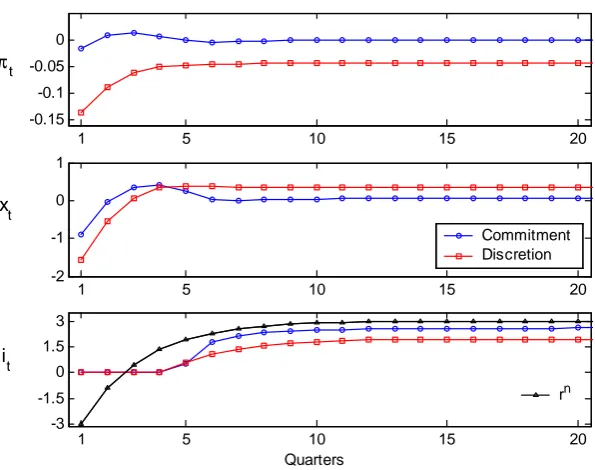
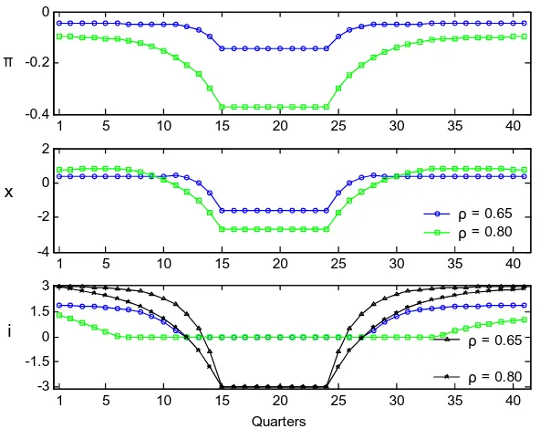
experiment is shown in gure 1.9, which plots a simulated “liquidity trap” under the

two regimes. The line with triangles in the bottom panel is the assumed evolution of

the natural real rate. It slips down from +3 percent (its deterministic steady-state) to -3

percent over a period of 15 quarters, then remains at -3 percent for 10 quarters, before

recovering gradually (consistent with the assumed AR(1) process) to around +3 percent

in another 15 quarters.

The rst and the second panels of gure 1.9 show the responses of in ation and

the output gap under each of the two regimes. Not surprisingly, under the optimal

15 _{That the zero interest rate policy should terminate in the same quarter under commitment and under}

discretion is a coincidence in this experiment. The relative duration of a zero interest rate policy under commitment versus discretion depends on the parameters of the shock process as well as the particular realization of the shock.

16 _{Notice that agents observe only the current state but form expectations about the future evolution of}

(32)

commitment regime both in ation and the output gap are closer to target than under the

optimal discretionary policy. In particular, under optimal discretionary policy in ation

is always below the target as it falls to -0.15% shadowing the drop in the natural real

rate. Compared to that, under optimal commitment prices are almost fully stabilized,

and in fact they even slightly increase while the natural real rate is negative. In turn,

under discretionary optimization the output gap is initially around +0.4% but then it

declines sharply to -1.6% with the decline in the natural real rate. In contrast, under

optimal commitment, output is initially at its potential level and the largest negative

output gap is only half the size of the one under optimal discretionary policy.

Supporting these paths of in ation and the output gap are corresponding paths

for the nominal interest rate. Under discretionary optimization the nominal rate starts

at around 2% and declines at an increasing rate until it hits zero two quarters before

the natural real rate has turned negative. It is then kept at zero while the natural real

rate is negative, and only two quarters after the latter has returned to positive territory

does the nominal interest rate start rising again. Nominal rate increases following the

liquidity trap mirror the decreases while approaching the trap, so that the tightening

is more aggressive in the beginning and then gradually diminishes as the nominal rate

approaches its steady-state.

In contrast, the nominal rate under optimal commitment begins closer to 3%, then

declines to zero one quarter before the natural real rate turns negative. After that, it

is kept at its zero oor until three quarters after the recovery of the natural real rate

to positive levels, that is one quarter longer compared to optimal discretionary policy.

Interestingly, once the central bank starts increasing the nominal rate, it raises it very

(33)

1.5 Targeting Rules with Zero Floor 24

is equivalent to six consecutive monthly increases by 50 basis points each. The reason

is that once the central bank has validated the in ationary expectations it has created

(helping mitigate de ation during the liquidity trap), there is no more incentive (and it

is costly) to keep in ation above the target.

Under discretion, the paths of in ation, output and the nominal rate are symmetric

with respect to the midpoint of the simulation period because optimal discretionary

policy is independent of history. Therefore, in ation and the output gap inherit the

dynamics of the natural real rate, the only state variable on which they depend. This is

in contrast with the asymmetric paths of the endogenous variables under commitment,

re ecting the optimal history dependence of policy under this regime. In particular,

the fact that under commitment the central bank can promise higher output gap and

in ation in the wake of a liquidity trap is precisely what allows it to engage in less

preemptive easing of policy in anticipation of the trap, and at the same time deliver a

superior in ation and output gap performance compared to the optimal policy under

discretion.

1.5 Targeting Rules with Zero Floor

In the absence of the zero oor, targeting rules take the form

Et t+j + xEtxt+k+ iEtit+l= ; (1.27)

where ; x; iare weights assigned to the different objectives,j; kandlare

forecast-ing horizons, and is the target. These are sometimes called exiblein ation targeting

(34)

1.5 Targeting Rules with Zero Floor 25

j; kor l > 0;the rules are called in ationforecast targeting to distinguish them from

targeting contemporaneous variables.

As demonstrated by (1.19) in section 1.3, in general such rules are not consistent

with the zero oor for they would require negative nominal interest rates at times. A

natural way to modify targeting rules so that they comply with the zero oor is to write

them as a complementarity condition,

it( Et t+j + xEtxt+k+ iEtit+l ) = 0 (1.28)

it 0

which requires that either the target is met, or else the nominal interest rate should

be bounded below by zero. In this sense, a rule like (1.28) can be labelled “ exible

in ation targeting with a zero interest rate oor”.

In fact, section 1.3 showed that the optimal policy under discretion takes this form

with i = 0; = ; x = ; j =k = 0;and = 0;namely

it xt+ t = 0 (1.29)

it 0

In the absence of the zero oor it is known that optimal commitment policy can

be formulated as optimal “speed limit targeting”,

xt+ t= 0; (1.30)

where xt = yt ytnis the growth rate of actual output relative to the growth rate

of its natural ( exible price) counterpart (the “speed limit”). In contrast to discretionary

optimization however, the optimal commitment rule with zero oor cannot be written

(35)

par-1.5 Targeting Rules with Zero Floor 26

ticular type of history dependence as shown by Eggertsson and Woodford (2003)17_{. In}

particular, manipulating the rst order conditions of the optimal commitment problem,

one can arrive at the following speed limit targeting rule with zero oor:

it xt+ t

1 +

1t 1 1t+

1

1t 1 = 0 (1.31)

it 0:

Since the product is small and is close to one, and for plausible (small)

values of 1tconsistent with the assumed stochastic process for the natural real rate, the

above rule can be approximated by

it

h

yt+ t t

i

= 0 (1.32)

it 0:

where t ytn+

1 2

1t is a history-dependent target (speed limit). In normal

circumstances when ₁_t = ₁_t ₁ = ₁_t ₂ = 0; the target is equal to the growth rate

of exible price output, as in the problem without zero bound; however if the

econ-omy falls into a liquidity trap, the speed limit is adjusted in each period by the speed

of change of the penalty (the Lagrange multiplier) associated with the non-negativity

constraint. The faster the economy is plunging into the trap, therefore, the higher is the

speed limit target which the central bank promises to deliver in the future, contingent

on the natural interest rate's return to positive territory.

While the above rule is optimal in this framework, it is not likely to be very

practical. Its dependence on the unobservable Lagrange multipliers makes it very hard

to implement or communicate to the public. Moreover, as pointed out by Eggertsson

17 _{These authors derive the optimal commitment policy in the form of a moving}_{price level}_targeting

(36)

1.6 Simple Instrument Rules with Zero Floor 27

and Woodford (2003), credibility might suffer if all that the private sector observes

is a central bank which persistently undershoots its target yet keeps raising it for the

following period. To overcome some of these drawbacks Eggertsson and Woodford

(2003) propose a simpler constant price level targeting rule, of the form

it

h

xt+ pt

i

= 0 (1.33)

it 0

whereptis the log price level.18

The idea is that committing to a price level target implies that any undershooting

of the target resulting from the zero oor is going to be undone in the future by positive

in ation. This raises private sector expectations and eases de ationary pressures when

the economy is in a liquidity trap. Figure 1.10 demonstrates the performance of this

simpler rule in a simulated liquidity trap. Notice that while the evolution of the nominal

rate and the output gap is similar to that under the optimal discretionary rule, the path of

in ation is much closer to the target. Since the weight of in ation in the central bank's

loss function is much larger than that of the output gap, the fact that in ation is better

stabilized accounts for the superior performance of this rule in terms of welfare.

1.6 Simple Instrument Rules with Zero Floor

The practical dif culties with communicating and implementing optimal rules like (1.31)

or even (1.33) have led many researchers to focus on simple instrument rules of the type

proposed by Taylor (1993). These rules have the advantage of postulating a relatively

18 _{Notice that the weight on the price level is optimal within the class of constant price level targeting}

rules. In particular, it is related to = =";the degree of monopolistic competition among intermediate

(37)

straightforward relationship between the nominal interest rate and a limited set of

vari-ables in the economy. While the advantage of these rules lies in their simplicity, at the

same time - absent the zero oor - some of them have been shown to perform close

enough to the optimal rules in terms of the underlying policy objectives (Galí 2003).

Hence, it has been argued that some of the better simple instrument rules may serve as

a useful benchmark for policy, while facilitating communication and transparency.

In most of the existing literature, however, simple instrument rules are speci ed

as linear functions of the endogenous variables. This is in general inconsistent with the

zero oor because for large enough negative shocks (e.g. to prices), linear rules would

imply a negative value for the nominal interest rate. For instance, a simple instrument

rule reacting only to past period's in ation,

it=r + + ( t 1 ); (1.34)

wherer is the equilibrium real rate, is the target in ation rate, and is an in ation

response coef cient, can clearly imply negative values for the nominal rate.

In the context of liquidity trap analysis a natural way to modify simple instrument

rules is to truncate them at zero with themax( ) operator. For example, the truncated

counterpart of the above Taylor rule can be written as

it= max [0; r + + ( t 1 )]: (1.35)

In what follows I consider several types of truncated instrument rules, including:

1. Truncated Taylor Rules (TTR) that react to past, contemporaneous or expected

future values of the output gap and in ation (j = 1;0;1),

(38)

2. TTR rules with partial adjustment or “interest rate smoothing” (TTRS),

iT T RS_t = max 0; _iit 1+ (1 i)i T T R

t (1.37)

3. TTR rules that react to the pricelevelinstead of in ation (TTRP),

iT T RP_t = max [0; r + (pt p ) + xxt] (1.38)

whereptis the log price level andp is a constant price level target; and

4. Truncated “ rst-difference” rules (TFDR) that specify thechange in the interest

rate as a function of the output gap and in ation,

iT F DR_t = max [0; it 1+ ( t ) + xxt]: (1.39)

The last formulation ensures that if the nominal interest rate ever hits zero it will

be held there as long as in ation and the output gap are negative, thus extending the

potential duration of a zero interest rate policy relative to a truncated Taylor rule.

I illustrate the performance of each family of rules by simulating a liquidity trap

and plotting the implied paths of endogenous variables under each regime. The

evalua-tion of average performance and uncondievalua-tional welfare is left for the following secevalua-tion.

Given the model's simplicity the focus here is not on nding the optimal values of

the parameters within each class of rules but rather on evaluating the performance of

al-ternative monetary policy regimes. To do that I use values of the parameters commonly

estimated and widely used in simulations in the literature. I make sure that the

para-meters satisfy a suf cient condition for local uniqueness of equilibrium. Namely, the

parameters are required to observe the so-called Taylor principle according to which the

nominal interest rate must be adjusted more than one-to-one with changes in the rate of

(39)

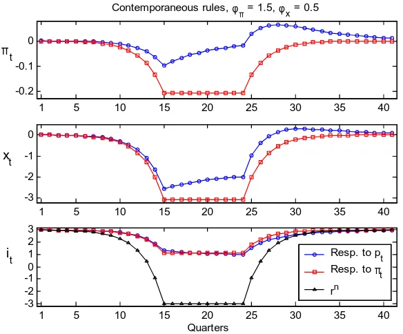
Figure 1.11 plots the dynamic paths of in ation, the output gap and the nominal

interest rate which result under regimes TTR and TTRP, conditional on the same path

for the natural real rate as before. Both the truncated Taylor rule (TTR, lines with

squares) and the truncated rule responding to the price level (TTRP, lines with circles)

react contemporaneously with coef cients = 1:5and _x = 0:5;and = 0.

Several features of these plots are worth noticing. First of all, and not surprisingly,

under the truncated Taylor rule, in ation, the output gap, and the nominal rate inherit

the behavior of the natural real rate. Perhaps less expected though, while both in ation

and especially the output gap deviate further from their targets compared to the optimal

rules in gure 1.9, the nominal interest rate stays always above one percent, even when

the natural real rate falls as low as -3 percent! This suggests that - contrary to popular

belief - an equilibrium real rate of 3% may provide a suf cient buffer from the zero

oor even with a truncated Taylor rule targeting zero in ation.

Secondly, gure 1.11 demonstrates that in principle the central bank can do even

better than TTR by reacting to the price level rather than to the rate of in ation. The

rea-son for this is clear - by committing to react to the price level the central bank promises

to undo any past disin ation by higher in ation in the future. As a result when the

econ-omy is hit by a negative real rate shock current in ation falls by less because expected

future in ation increases.

Figure 1.12 plots the dynamic paths of endogenous variables under regimes TTRS

and TFDR, again with = 1:5; _x = 0:5 and = 0. TTRS (lines with circles)

is a partial adjustment version of TTR, with smoothing coef cient i = 0:8: TFDR

(line with squares) is a truncated rst-difference rule which implies more persistent

(40)

1.7 Welfare Ranking of Alternative Rules 31

The gure suggests that interest rate smoothing (TTRS) may improve somewhat

on the truncated Taylor rule (TTR), and may do a bit worse than the rule reacting to

the price level (TTRP). However, it implies the least instrument volatility. On the other

hand, the truncated rst-difference rule (TFDR) seems to be doing the best job at

stabi-lization in a liquidity trap among the examined four simple instrument rules. However,

under this rule the nominal interest rate deviates most from its steady-state, hitting zero

for ve quarters. Interestingly, the paths for in ation and the output gap under this rule

resemble, at least qualitatively, those under the optimal commitment policy. This

sug-gests that introducing a substantial degree of interest rate inertia may be approximating

the optimal history dependence of policy implemented by the optimal commitment rule.

It is important to keep in mind that the above simulations are conditional on one

particular path for the natural real rate. It is of course possible that a rule which appears

to perform well while the economy is in a liquidity trap, turns out to perform badly “on

average”. In the following section I undertake the ranking of alternative rules according

to an unconditional expected welfare criterion, which takes into account the stochastic

nature of the economy, time discounting, as well as the relative cost of in ation vis-a-vis

output gap uctuations.

1.7 Welfare Ranking of Alternative Rules

A natural criterion for the evaluation of alternative monetary policy regimes is the

cen-tral bank's loss function. Woodford (2003) shows that under appropriate assumptions

the latter can be derived as a second order approximation to the utility of the

represen-tative consumer in the underlying sticky price model.19 _{Rather than normalizing the}

(41)

weight of in ation to one, I normalize the loss function so that utility losses arising

from deviations from the exible price equilibrium can be interpreted as a fraction of

steady-state consumption,

W L = U U

UcC

= 1 2E0

1

X

t=0

t

"(1 +'") 1 2_t + 1+' x2_t

= 1

2"(1 +'")

1 E0

1

X

t=0

t

Lt (1.40)

where = 1(1 ) (1 ) ; is the fraction of rms that keep prices unchanged in

each period,'is the (inverse) elasticity of labor supply, and"is the elasticity of

substi-tution among differentiated goods. Notice that( 1₊_'_{) [}_"_{(1 +}_'"_)] 1

= =" =

implies the last equality in the above expression, whereLtis the central bank's period

loss function, which is being minimized in (1.3).

I rank alternative rules on the basis of the unconditional expected welfare. To

compute it, I simulate 2000 paths for the endogenous variables over 1000 quarters and

then compute the average loss per period across all simulations. For the initial

distrib-ution of the state variables I run the simulation for 200 quarters prior to the evaluation

of welfare. Table 1.2 ranks all rules according to their welfare score. It also reports the

volatility of in ation, the output gap and the nominal interest rate under each rule, as

well as the frequency of hitting the zero oor.

A thing to keep in mind in evaluating the welfare losses is that in the benchmark

model with nominal price rigidity as the only distortion and a shock to the natural real

rate as the only source of uctuations, absolute welfare losses are quite small - typically

less than one hundredth of a percent of steady-state consumption for any sensible

(42)

etary policy regime.20 _{Therefore, the focus here is on evaluating rules on the basis of}

their welfare performancerelativeto that under the optimal commitment rule.

In particular, in terms of unconditional expected welfare, the optimal

discre-tionary policy (ODP) delivers losses which are nearly eight times larger than the ones

achievable under the optimal commitment policy (OCP). Recall that abstracting from

the zero oor and in the absence of shocks other than to the natural real rate, the

out-come under discretionary optimization is the same as under the optimal commitment

rule. Hence, the cost of discretion is substantially understated in analyses which ignore

the existence of the zero lower bound on nominal interest rates. Moreover,conditional

on the economy's fall into a liquidity trap the cost of discretion is even higher.

Interestingly, the frequency of hitting the zero oor is quite high - around one

third of the time under both optimal discretionary and optimal commitment policy. This

however depends crucially on the central bank's targeting zero in ation in the baseline

model without indexation. If instead the central bank targets a rate of in ation of, say

2%, the frequency of hitting the zero oor would decrease to around 12% of the time

(which is still higher than what is observed in the US).

Table 1.2 further con rms Eggertsson and Woodford (2003) intuition about the

desirable properties of an (optimal) constant price level targeting rule (PLT) - here losses

are only 56% greater than those under the optimal commitment rule. It also involves

hitting the zero oor around one third of the time.

In comparison, losses under the truncated rst-difference rule (TFDR) are 7.5

times as large as those under the optimal commitment rule (even though its performance

in a liquidity trap seemed comparable to that of PLT). Interestingly, however, TFDR

20 _{To be sure, output gaps in a liquidity trap are considerable; however the output gap is attributed}

(43)

OCP PLT TFDR ODP TTRP TTRS TTR std( )x 102 _1.04 _3.47 _4.59 _3.85 _7.23 _9.12 _12.9

std(x) 0.45 0.69 1.04 0.71 1.61 1.91 1.90

std(i) 3.21 3.20 1.36 3.27 1.06 0.56 1.14

Loss x 105 _6.97 _10.9 _52.3 _54.2 _62.9 ₁₀₃ ₁₄₇

Loss/OCP 1 1.56 7.50 7.77 9.01 14.8 21.1

Pr(i= 0) % 32.6 32.0 1.29 36.8 0.24 0.00 0.44

Table 1.2. Properties of Optimal and Simple Rules with Zero Floor

narrowly outperforms optimal discretionary policy. Even though the implied volatility

of in ation and the output gap is slightly higher under this rule, it does a better job than

ODP at keeping in ation and the output gap closer to target on average. An additional

advantage - albeit one that is not re ected in the benchmark welfare criterion - is that

instrument volatility is less than half of that under any of the policies ODP, OCP or PLT.

This implies that the zero oor is hit only around 1.3% of the time under this rule.

Similarly, losses under the truncated Taylor rule reacting to the price level (TTRP)

are nine times larger than under OCP, and only slightly worse than optimal discretionary

policy. Moreover, instrument volatility under this rule is smaller than under TFDR,

which implies hitting the zero oor even more rarely - only one quarter every 100 years

on average.

The rule with the least instrument volatility among the studied simple rules - less

than one- fth of that under OCP - is the truncated Taylor rule with smoothing (TTRS).

As a consequence, under this rule the nominal interest rate virtually never hits the zero

lower bound. However, welfare losses are almost fteen times larger than under OCP.

Finally, under the simplest truncated Taylor rule (TTR) without smoothing the

zero lower bound is hit only two quarters every 100 years, while welfare losses are

around 20 times larger than those under OCP. Nevertheless, even under this simplest

(44)

1.8 Sensitivity Analysis 35

The fact that the zero lower bound is hit so rarely under the four simple instrument

rules suggests that the zero constraint may not be playing a big role for unconditional

expected welfare under these regimes. Indeed, computing their welfare score without

the zero oor (by removing the max operator), reveals that close to 99% of the welfare

losses associated with the four simple instrument rules stem from their intrinsic

sub-optimality rather than from the zero oor per se. Put differently, if one reckons that

the stabilization properties of a standard Taylor rule are satisfactory in an environment

in which nominal rates can be negative, then adding the zero lower bound to it leaves

unconditionally expected welfare virtually unaffected. Nevertheless, as was illustrated

in the previous section, conditional on a negative evolution of the natural real rate,

the losses associated with most of the studied simple instrument rules are substantially

higher relative to the optimal policy.

1.8 Sensitivity Analysis

In this section I analyze the sensitivity of the main ndings with respect to the

parame-ters of the shock process, the strength of reaction and the timing of variables in truncated

Taylor-type rules, and an extension of the model with endogenous in ation persistence.

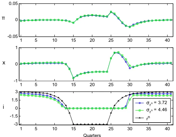
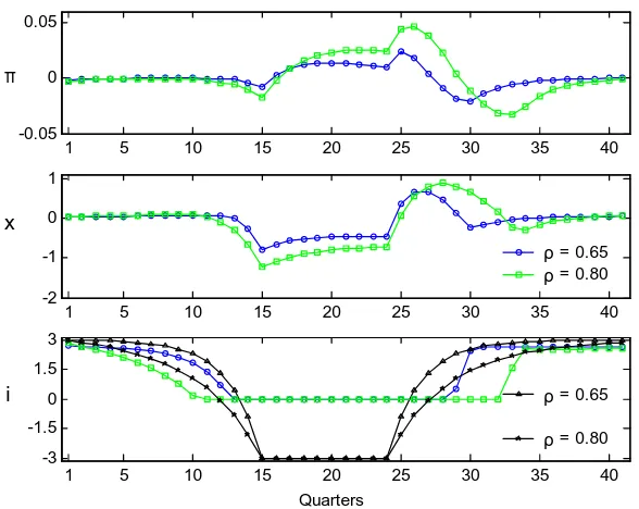
1.8.1 Parameters of the Natural Real Rate Process

Larger variance

Table 1.3 reports the effects of an increase of the standard deviation of rn _to