Essays in international finance

(1)

Essays in International Finance

Gonçalo Pina

TESI DOCTORAL UPF / 2012

DIRECTOR DE LA TESI

Prof. Jaume Ventura

(2)

(3)

(4)

(5)

Acknowledgments

I thank my supervisor Jaume Ventura for his continuous support and

couragement. Not only did he patiently teach me how to conduct and

en-joy research in economics, he also guided me through some difficult deci-sions. For this I am deeply grateful. Faculty and colleagues at CREi and

UPF made for an exciting research environment and I benefited immensely

from interacting with them. I thank Paulo Abecasis, Diederik Boertien, Fernando Broner, Paula Bustos, Vasco Carvalho, Nicola Gennaioli, Timo

Hiller, Gueorgui Kolev, Alberto Martin, Romain Ranci`ere, Sandro

Shele-gia, Hans-Joachim Voth, Sander Wagner, Robert Zymek, and many other participants in the CREi International Lunch, assorted meetings and breaks

for their comments and suggestions.

Marta Araque and Laura Augusti played a crucial role with their adminis-trative assistance. I thank them for their help and infinite patience.

Finally, I would like to thank my friends, my family and Mona. I would not

have made it without them.

(6)

(7)

(8)

Abstract

This thesis investigates two economic policy dimensions in contemporary

world economy. The first chapter focuses on the recent accumulation of

in-ternational reserves by central banks in developing economies. I present a simple model of reserve management where a central bank accumulates

re-serves in order to avoid spikes in inflation during financial crises. This

mon-etary perspective helps to account for the massive accumulation of reserves observed in the data. The second chapter turns to financial reform, with an

emphasis on the role played by savings. I show how imperfect competition

in the financial sector can internalize externalities and yield larger invest-ment when domestic savings are low. Taking this view allows for a better

understanding of the empirical relationship between financial reforms and

economic growth.

Res ´

umen

Aquesta tesi investiga dues dimensions de la poltica económica en l’economia mundial contemporània. El primer cap´ıtol es centra en la recent acumulació

de reserves internacionals per part dels bancs centrals en les economies

en desenvolupament. Exposo un model senzill de gesti´o de reserves per part d’un banc central que acumula reserves amb l’objectiu d’evitar els

augments pronunciats d’inflaci´o durant les crisis financeres. Aquesta

per-spectiva monet`aria ajuda a explicar l’acumulaci´o massiva de reserves que s’observa en les dades. El segon cap´ıtol es focalitza en la reforma financera,

emfasitzant el paper de l’estalvi. Demostro com la compet`encia imperfecta

en el sector financer pot internalitzar les externalitats i aix´ı generar més in-versió, concretament quan l’estalvi és baix. L’adopció d’aquest punt de vista

permet entendre millor la relaci´o emp´ırica entre les reformes financeres i el

(9)

(10)

(11)

Foreword

This dissertation consists of two essays in international finance. Each chap-ter focuses on a different policy dimension that is of particular relevance for

developing economies.

The first chapter studies the recent increase in international reserves hold-ings in developing economies, a phenomenon that has been puzzling

aca-demics and policy makers in the last decades (Jeanne 2007). This paper

ex-plores the view that international reserves are the outcome of optimal policy from a central bank that wishes to smooth inflation. Inflation is distortionary,

but the central bank needs to raise inflation-related revenues. These revenue

needs are exceptionally large during financial crises. As a result, the cen-tral bank optimally accumulates international reserves in order to spread the

distortions associated with inflation over time. A quantitative exercise for

an average developing economy using data between 1970 and 2007 predicts long-run levels of reserves that coincide with average holdings in

develop-ing economies. Furthermore, the model delivers predictions for exchange

rates that mirror the data: (i) exchange rates depreciate while the central bank accumulates reserves; (ii) if a country has accumulated a large amount

of reserves, exchange rates do not drastically depreciate during a financial

crisis. Finally, the monetary perspective studied in this paper sheds light on the determinants of cross-sectional variation in reserve holdings.

The second chapter investigates the optimal portfolio of financial reforms.

This chapter shows that between 1973 and 2005, many countries decided to implement macro reforms (defined as the liberalization of prices and

quantities in financial markets), but not micro reforms (reforms targeting

the participants and competition in financial markets). Interestingly, coun-tries performing macro reforms grew less when compared to councoun-tries that

implemented both reforms simultaneously. I explore a second best view of

financial liberalization and show theoretically under which conditions per-forming macro financial reforms without micro financial reforms increases

investment. The first best is sometimes not attainable due to the interaction

(12)

external-ity. In particular, this is the case when domestic savings are low relative to financial intermediation. In the empirical analysis, I show that accounting

for differences in savings rates contributes to our understanding of the effect

of different portfolios of financial reforms on growth.

Taken together, these chapters highlight the role of second best policies in a

world of imperfect financial markets. In the first chapter, reserve

accumula-tion is a costly response to insufficient internaaccumula-tional insurance for financial risks. In the second chapter, restricting competition in the financial sector is

a costly alternative to a world of volatile capital flows and contract

enforce-ment crises. The recent financial crisis has spurred a growing literature on financial policy in open economies. This dissertation adds to this exciting

(13)

(14)

Chapter 1 The Recent Growth of International Reserves in

Developing Economies: A Monetary Perspective

1.1 Introduction

The last 20 years have witnessed a large increase in international reserve

holdings by central banks in developing economies. Figure 1.1 plots the evolution of reserves for developed and developing economies as a share

of theirGDP between 1970 and 2007.1 The most striking feature of this graph is the divergence between the two groups of countries between 1987

and 2007. Following a relatively stable period of reserves toGDPratios

close to 10%, since 1987 developed economies have been reducing their reserves relative toGDP. At the same time, developing economies have

steadily increased their international reserves relative toGDPto a level that

exceeded 25% in 2007.

Why have central banks in developing countries increased their reserve

hold-ings, in contrast to their developed-country counterparts? This accumulation has important implications. From the perspective of a developing economy,

it represents foregone consumption and investment in countries with good

growth prospects. From the perspective of the global economy, reserves have played a role in the emergence of upstream capital flows - from poor

1_{International reserves are defined as liquid external assets under the control of the central}

(19)

[image:19.499.140.363.75.233.2]

Figure 1.1: Unweighted cross-country averages of International Reserves as a share of GDP for 24 developed economies and 154 developing economies between 1970-2007. Source: author’s calculations based on the updated and extended version of the dataset constructed by Lane and Milesi-Ferretti (2007).

to rich countries - and contributed to global imbalances. This paper takes a monetary view on this phenomenon and argues that the desire of central

banks to smooth inflation together with their financial responsibilities

dur-ing bankdur-ing crises can explain observed reserve holddur-ings.

I set up the problem of a central bank that has to finance exogenous and stochastic spending shocks with inflation. Inflation is distortionary and the

central bank wishes to spread distortions over time. To do so, it accumulates

reserves in order to smooth inflation against these shocks. Central bank spending shocks are particularly large during banking crises. Using data

between 1970−2007, I find that the long-run level of reserves for an average developing economy predicted by the model amounts to 21% ofGDP.

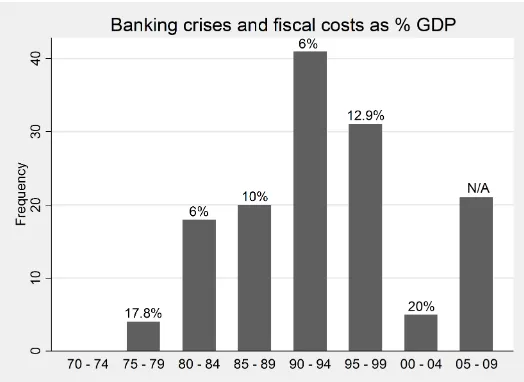
Figure 1.2 plots the incidence of banking crises in the last 40 years. The

gray bars plot the frequency of banking crises in the world economy

dur-ing 5-year windows. These crises were particularly frequent in the last 20 years.2 Banking crises were also very costly. The numbers on top of the

2_{Reinhart and Rogoff (2008) show that banking crises are not exclusive to the last two}

(20)

[image:20.499.118.380.70.261.2]

Figure 1.2: Frequency of crises and median fiscal cost (gross, as % ofGDP; N/A: not available) between 1970-2010. Measure for fiscal cost is only available for selected crises. Source: Laeven and Valencia (2008, 2010).

gray bars represent the median fiscal cost of banking crises in percentage of

GDPfor each 5-year window. Furthermore, a substantial fraction of these

fiscal shocks are financed by the central bank with inflation related revenues.

Available estimates amount to 10% ofGDP, in episodes where the total fis-cal cost ranges between 15 and 65% ofGDP.3

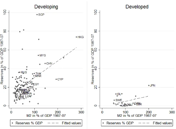
Ultimately, what matters for the central bank are prospective crises, not

real-ized crises. Figure 1.3 plots reserves against a measure of size of the

finan-cial sector between 1987−2007 for developed and developing economies. There is a clear positive relationship between reserves and size of the

finan-cial sector. In this paper I argue that, starting in the late 1980s, the need to provide banking sector support in periods of crisis required a new

as-crises across the world economy. They associate these events to increases in capital mobility (see Figure 3 in their paper).

3_{See Burnside et al (2001, 2006) for estimation of inflation related revenues. Looking at}

(21)

sessment of international reserves adequacy by central banks in developing economies.4,5

It is instructive to look at one of these developing economies. Figure 1.4

plots at the evolution of Reserves,M2 (as a measure of size of the financial

sector) and inflation in Korea between 1987 and 2010, together with the timing of the Korean 1997 banking crisis and the Global 2007-09 crisis.

Section 1.5 goes into more detail into these two episodes but it is noteworthy

to see that even for the annual data presented in Figure 1.4, in both crises reserves decreased relative to output. This reduction was stronger in the

2007 crisis, although this episode was not classified as a banking crisis in

Korea (Laeven & Valencia (2010)). One important difference in 2007-08, was that the Korean central bank had now amassed a large stock of reserves.

This picture also shows the upward trend in the size of the financial sector as measured byM2/GDP, and a downward trend in inflation. These two

come associated with a large increase in reserves as a share ofGDP. In both

crises, inflation increases as reserves decrease.6

The model also predicts exchange rate behavior that is consistent with the evidence. Large stocks of international reserves have been associated with

undervalued exchange rates. In the model, the central bank accumulates

in-4_{Empirical research has noted the correlation between the size of the financial sector and}

reserves. Burke and Lane (2001) are the first to document the correlation between M2/GDP and reserves in a purely cross sectional analysis. Obstfeld et al (2010) perform a panel analysis and argue that in developing economies M2/GDP causes reserves and that managed exchange rate mechanisms are correlated with reserves. They interpret reserves as savings to support the banking sector through bailouts while avoiding currency depreciation.

5_{There are other policies that countries can take to avoid banking crises. For example,}

prudential regulation. In this paper, I take these as exogenous to the actions of the central bank.

6_{Consider first the 1997 crisis. Burnside et al (2006) estimate the amount financed by}

(22)

[image:22.499.107.396.69.280.2]

Figure 1.3: International Reserves as a share of GDP and size of the financial sector (measured byM2/GDP) for developing and developed economies between 1987-2007. Sources: Lane and Milesi-Ferretti (2007) and WDI.

ternational reserves resorting to inflation.7 As a consequence, the value of

domestic currency decreases relative to foreign currencies. In other words, the nominal exchange rate depreciates during the accumulation process.

When a crisis occurs, the central bank deploys its reserves to finance the banking sector support. This sustains the value of domestic currency and

keeps the exchange rate from collapsing.8

The view explored in this paper can shed light on the divergence between

the two groups of economies in Figure 1.1. Developed economies are less dependent on international reserves because(i) they rely less on inflation

related revenues, and(ii)their central banks have access to contingent

bor-rowing in times of crisis. There is also substantial heterogeneity within

7_{The model abstracts from the role of sterilization policy, by assuming that domestic}

debt and foreign debt are perfect substitutes for domestic agents. This implies that printing money is always inflationary. See Brutti (2011) and Gennaioli et al (2010) for open economy models where domestic agents prefer to hold domestic government bonds.

8_{Aizenman and Sun (2009) and Dominguez et al (2011) show that countries drew from}

(23)

Figure 1.4: Annual data on Reserves and M2 as a share ofGDP, and infla-tion for Korea between 1987 - 2010. Data from IFS.

countries that accumulate reserves. Although most developing countries

have accumulated international reserves, Figure 1.1 masks substantial

cross-sectional variation. Figure 1.3 illustrates this point by plotting the aver-age ratio of reserves to GDPbetween 1987 and 2007 for both groups of

countries on they-axis. This heterogeneity is less present for developed economies.

In the quantitative section of the paper I perform a series of exercises to study the sources of cross-sectional variation in reserve accumulation. I find

that the most important determinant of the stock of international reserves is

the size of a crisis. The frequency with which crises occur is less impor-tant. This indicates that countries with larger banking sectors should have

more international reserves. The other crucial determinant of reserves is

the relative importance of distortions. I highlight two distortions in this pa-per: inflation distorts the consumption/savings and the investment decisions

of households. The investment distortion is particularly disruptive since in

the open economy setting used in this paper, capital is more elastic than consumption. Inflation can not distinguish between capital and

consump-tion. As a consequence, countries where the investment distortion is more

(24)

analysis confirms that countries with less developed financial markets, and lower access to credit, have larger stocks of reserves. This distinction

be-tween size and financial development is important to understand the

cross-sectional variation of international reserves within developing economies.

The recognition that reserve holdings are a crucial instrument for policy in

open economy models dates back to the literature on balance of payments

crises in economies with fixed exchange rates - notably, Krugman (1979), Flood and Garber (1984) and Broner (2009). In these papers, the level

of reserves determines the duration of an unsustainable exchange rate peg.

Calvo (1987) provides microeconomic foundations and studies the dynam-ics of balance of payments crises in an economy with maximizing agents

that demand money due to a cash-in-advance constraint. Subsequent work by Burnside et al (2001), Kumhof et al (2010), Rebelo and Veigh (2008)

and Rigobon (2002) analyzes economic policy in this model.9 Although

these papers study policy, they take the central bank’s holdings of reserves at the moment of the crisis as exogenous. In other words, there is no reserve

accumulation in place. The main differences in my paper are that I study

an economy that is not yet in crisis, and where the central bank takes into account the magnitude of a prospective crisis and the distortions associated

with inflation when accumulating international reserves.10

A recent literature studies optimal accumulation of international reserves as

9_{Burnside et al (2001) argue that the Asian crisis of 1997 was caused by prospective}

deficits associated with implicit guarantees to failing banks, to be financed with inflation related revenues. The reserve accumulation model I explore in this paper shares the same perspective on monetary policy. Faced with the possibility of future deficits, but in a situation with strong economic conditions, a central bank accumulates reserves to avoid future large swings in inflation and exchange rates. Kumhof et al (2010) extends the analysis to different ad-hoc inflation and exchange rate mechanisms to explore their quantitative implications. Rebelo and Vegh (2008) study the optimal time to abandon a fixed exchange rate mechanism. Rigobon (2002) studies the problem of a central bank that draws from its reserves to reap benefits from a future fiscal reform.

10_{It is important to mention that the focus on the inflation tax is a simplification. For}

(25)

precautionary savings or insurance in order to smooth aggregate consump-tion. This perspective, developed by Alfaro and Kanczuk (2009), Durdu

et al (2009) and Jeanne and Ranci`ere (2010), considers that developing

economies depend on short-term capital inflows. Countries accumulate re-serves to sustain consumption when there are negative output shocks and

access to international financial markets is interrupted, a view that has been

synthesized by the celebrated Guidotti-Greenspan rule.11 However, quan-titative versions of these models cannot account for the observed level of

reserves.12 Furthermore, this literature points to short term debt as a

cru-cial determinant of reserves. But in the data short term debt is not strongly correlated with reserves.13

The monetary perspective presented in this paper shares the view that re-serves are held due to insurance or precautionary motives. But there are

important differences with the consumption smoothing literature. I focus on the problem of one big agent, the central bank, that interacts with the rest

of the economy. On the contrary, the literature on consumption smoothing

summarizes the whole economy as one single agent. This literature is im-plicitly assuming that resources can be allocated within the economy in a

non-distortionary way.14 My paper shows that heterogeneity plays a crucial

role. The shocks I consider affect disproportionally one part of the econ-omy, the central bank. Also, the mechanism to transfer resources within the

economy - inflation - is distortionary. Together, these assumptions provide a

different reason for central banks to hold reserves that has been overlooked so far. International reserves are a way to smooth the distortions associated

with transferring resources within the economy.15

11_{The Guidotti-Greenspan rule states that the ratio of reserves to short term debt should}

be 1 (Greenspan (1999)).

12_{Jeanne and Ranci`ere (2010) find that reserves should be 9}_._{1% of GDP, Durdu et al}

(2009) find 9.61%, whereas Alfaro and Kanczuk (2009) find 0%. These are much smaller than the 25.8% shown in Table A.4.1 (Appendix A.4) and Figure 1.1.

13_{See Obstfeld et al (2010) and Section 1.4 of this paper.}

14_{To make this point clear, I show that a model of consumption smoothing obtains the}

same reserves levels as a model of inflation smoothing when inflation is non-distortionary. 15_{Aizenman and Marion (2004) study political-economy considerations in an ad-hoc}

(26)

These features are ultimately related to the literature on tax smoothing in-troduced by Barro (1979). In Barro’s economy, the optimal tax policy is for

the government to smooth taxes over time. This policy is the consequence

of convex costs associated with distortionary taxes. I take this insight and embed it in a monetary model. Importantly, this leads to a dramatic increase

in the level of international reserves predicted by the small open economy

model.

The paper proceeds as follows: Section 1.2 introduces the monetary model and describes the central bank problem. In Section 1.3 I solve for a

deter-ministic example that allows for a closed form solution, and develop the

main intuitions of the model. Section 1.4 studies the quantitative predic-tions of the model. Section 1.5 looks at some case studies and performs a

cross-country empirical analysis on reserve accumulation. Finally, Section

1.6 concludes and points to future research.

1.2 A monetary model of reserve accumulation

The model extends Rigobon (2002) and Calvo (1987) with a focus on

re-serve accumulation. A representative consumer and a central bank use a non-contingent bond to smooth exogenous stochastic financing needs. I

fo-cus on the the problem of a central bank. The central bank dislikes

infla-tion but has financial responsibilities, demanded by the government.16 To finance them it can use two instruments: (i) it can raise inflation related

revenues or (ii) it can withdraw from its international reserves. Because

inflation is distortionary, the central bank wishes to spread the burden of in-flation across time. As a result, it accumulates reserves in non-crisis periods

and when necessary, uses a mix of inflation and reserves.

16_{These financial responsibilities take the form of financial sector support but are}

(27)

1.2.1 Setup

Consider a small open economy with one traded good. This good can be

used for consumption or investment. Time is continuous. There are two agents: an infinitely lived representative consumer and a central bank. At

any moment in time, the economy is either on a crisis state (H), or in a

non-crisis state (L). The difference between the two is the amount of funds demanded from the central bank. I now describe the problem of each agent

in this economy.

The representative consumer maximizes the expected lifetime utility from the consumption plan {ct}∞₀. The objective function of the consumer is

given by:

E₀

Z _∞

0

u(ct)e−βtdt (1.1)

where,

u(c) = c

1−σ₋₁

1−σ

andβ >0 is the discount factor. The consumer can invest in a production

technology, in a risk free foreign bond or in money holdings. Production features a Cobb-Douglas technology using capitalktand laborlt:F(kt,lt) =

Atktαl1

−α

t . The consumer has one unit of labor lt =1, α is the share of

capital and capital depreciates at rateδ. Then, investingkt units of capital

in domestic production yieldsAkα

t −δkt units of output.

In addition, the consumer has access to two assets. A foreign bond f earns

the foreign real interest rateρ, that is assumed to be constant. The consumer

can also invest in money holdingsMt. Money is introduced in this economy

through a cash-in-advance constraint on consumption and on the use of

cap-ital. This asset is useful for production and consumption purposes, but loses value with inflation. The opportunity cost of holding money is given by the

nominal interest rate, which corresponds to the loss of value due to

(28)

production technology or in the foreign bond.

LetPtbe the domestic price level att, andπt=

·

Pt

Pt the domestic inflation rate

(and let the international inflation rate be zero). I assume that purchasing power parity holds (PPP) such that the exchange rate is determined by

in-flation. Assume also that all debt is indexed to domestic inin-flation.17 Then,

the nominal domestic interest rate is given by:it=ρ+πt. The flow budget

constraint of the consumer can be written as:

·

ft+

·

Mt

Pt

+

·

kt =ρft+Aktα−δkt−ct (1.2)

Additionally, the consumer faces a cash-in-advance constraint. To consume

ct units of the consumption good and to operate the capital stock kt, he

must have real money holdings Mt

Pt at least larger than vcct+vkkt, where

(vc,vk) measure the constant amount of cash needed for consumption and

production services. The cash-in-advance constraint is given by:

vcct+vkkt≤

Mt

Pt

(1.3)

Defineat=ft+M_Pt

t +ktas the wealth of the consumer in real terms. Because

consumers only care about real balances, define real money balances asmt= Mt

Pt. As a store of value, money is always dominated by foreign assets if

it =πt+ρ ≥0, which I assume throughout. Thus, the cash-in-advance

constraint (1.3) will always hold with equality and money demand is given

bymt=vcct+vkkt. I can then rewrite the flow budget constraint as

·

at=ρat+Akαt −(1+vcit)ct−(δ+ρ+vkit)kt (1.4)

Finally, the consumer’s solvency condition is given by:

17_{This implies that domestic and foreign debt are perfect substitutes for the consumer and}

(29)

lim

t→∞

ate−βt ≥0 (1.5)

The problem of the consumer is then to choose a sequence of{ct}∞₀,{kt}∞₀,

so as to maximize (1.1), subject to the flow budget constraint (1.4) and the

solvency condition (1.5), given{it}∞₀, f0,k0andm0. Appendix A.1.1 shows

that the solution to the consumer problem is given by the following system of differential equations:

kt =

αA δ+ρ+vkit

₁₋1

α

(1.6)

∂ctj

∂at

≈1+vci j t · c j t σ ! ·  

ρ−β−qj 

 1−

1+vci j t

1+vci

−j t

c_tj

σ

c−_t jσ

     · _·

a_tj

−1

(1.7)

·

a_tj=ρat+A·

ktj

α

−1+vcitj

ctj−

δ+ρ+vkitj

ktj (1.8)

lim

a→∞

ctj=∞, j=L,H

(1.9)

Equation (1.6) shows that capital is determined by the international

inter-est rateρ, the depreciation rate δ and the domestic nominal interest rate that is relevant for the use of capital, vkit. Because there are free

move-ments of capital, at any periodt, the capital stock is obtained by equating marginal cost to marginal benefit. It follows from equation (1.6) that at any

periodt, production is maximized ifit is the lowest possible. This equation

summarizes the production side of the agent’s problem, and highlights the distortions in production caused by inflation.

There are two equations governing consumption and savings for each state

j=L,H, given by equations (1.7) and (1.8). The effect of the domestic

nominal interest rate on production is important for this decision, and it

is felt through equation (1.8). The solution to the consumer problem is

then defined by a family of curves for each pair of interest ratesi_tL,iH t

∞

(30)

depending on the state of the economy. For any given interest rate pair

i_tL,itH

, if the economy spends enough time in stateL, the consumer’s assets

will tend toa∗, defined as a situation where

·

aLt =0.

For a given interest rate policy, this model is a traditional small open

econ-omy model and can be used to study consumption, investment and capital flows. In this paper, I am interested in optimal interest rate policy and

re-serve management, and their implications for the aggregates in the economy.

We now turn to the problem of the central bank.

1.2.2 The central bank problem

I assume the central bank to be benevolent. It solves a constrained op-timization problem: subject to the demands of the government, the

con-sumer’s choices and it’s own budgetary constraints, the central bank

maxi-mizes the representative consumer’s utility. The solution is represented by a time-consistent contingent plan for the interest rate{it}∞₀ that maximizes

(1.1). Because the consumer demands real money balances, the central bank

can tax the consumer through inflation. With the resources obtained from

seigniorage

·

Mt

Pt , the central bank can pay for spendinggt or accumulate

in-ternational reservesrt that earn interestρ. Absent any borrowing constraint,

the central bank can also borrow from the international bond market at rate

ρ. However, since this asset is not contingent on shocks togt, the central

bank does not have access to perfect insurance.

The external budget constraint of the central bank is given by:

·

rt=ρrt+

·

Mt

Pt

−gt (1.10)

In exchange for the financinggt the central bank gets domestic debt, either

issued by the government or from financial institutions. The balance sheet

(31)

bt+rt=mt

where,bt+rtare the assets, andmtcorresponds to its liabilities. The budget

constraint of the central bank can be rewritten as:18

·

bt =ρbt+gt−(πt+ρ)mt (1.11)

The central bank may face a constraint on how much debt it can issue

abroad. I introduce this through an exogenous borrowing constraint given

byrt ≥r=0.

Note that the assumptions of PPP, indexed debt and perfect capital mobility

imply that choosing inflation πt is the same as choosing it. Since

inter-national inflation is zero, exchange rate depreciation tracks one to one the inflation rate. That is, when inflation increases, the value of the domestic

currency loses value and the exchange rate depreciates. When choosing the nominal interest rate, the central bank takes into account the impact of its

decisions on the representative consumer. In particular, the set of equations

given by (1.6)-(1.9) are constraints in the optimal policy problem of the cen-tral bank.

Absent any spending demands gt, the optimal policy of an unconstrained

central bank is given by the Friedman rule, withit=0 andπt =−ρ.

How-ever,gt will occasionally be quite large and the central bank will have to

resort to inflation. To keep the analysis simple, I study the case wheregt

takes one of two valuesgL,gH , and evolves according to the following Poisson process:

(32)

gt+dt=           

gL _w_.p. ₁₋_q

Ldt ifgt =gL

gH w.p. qLdt ifgt =gL

gH w.p. 1−qHdt ifgt=gH

gL w.p. qHdt ifgt=gH

(1.12)

This economy will be in one of two states of nature, defined bygH>>gL.

At any non-crisis period, a crisis arrives with probabilityqLand leaves with

probabilityqH. Because crises are relatively less frequent than safe periods,

qH >>qL. This framework captures in a parsimonious way the type of

shocks that I am studying: infrequent but severe crisis. We are now ready to

study the optimal policy problem. At anyt, the central bank takes as given

a0andb0and solves:19

max

{it}

E₀

Z ∞

0

u(ct)e−βtdt

s.t.

·

bt=ρbt+gt−itmt

·

at=ρat+Akαt −(1+vcit)ct−(δ+ρ+vkit)kt

rt=mt−bt

mt=vcct+vkkt

lim

T→∞

bTe−βT=0, a0,b0,

gt given by(1.12)

it≥0,rt ≥r

and equations(1.6)−(1.8)

Suppose the economy starts in a period with lowgt, but the central bank

knows it might face a crisis soon, and an increase in gt. In this simple

setting, the central bank can either print money or draw from its reserves.

19_{This model approximates a version of the model of consumption smoothing considered}

(33)

Printing money causes inflation which decreases consumption and distorts savings and investment. It follows that the optimal policy of the central bank

is to smooth inflation.

The extent to which it can smooth inflation depends on the existence of

con-straints on how much the central bank can borrow abroad.20 If the central

bank is unconstrained, the crisis will be financed mostly with future rev-enues and the central bank need not accumulate many reserves. On the

other hand, if there is a constraint, this limits the amount of future revenues

a central bank can transfer to the crisis period thus increasing precautionary savings ex-ante.

The optimal policy problem can be described with two value functions, one for each state j=L,H, subject to the relevant constraints. Given state j,

the relevant state variable of the economy is summarized by a pair of

do-mestic credit and assets of the representative agent(at,bt). There are four

constraints in the central bank problem. First, his budget constraint which

is summarized by equation (1.11). Second, the borrowing constraint on

re-servesrt≥r. There are two constraints coming from the consumer problem

represented by equations(1.6)−(1.8): the consumer budget constraint and

an equation that combines(1.6) and(1.7), which summarizes the optimal

consumption and investment decisions given the policy of the central bank. I represent the problem using the following value functions, where I omit

the subscriptstand the state variables to simplify notation:

βVL=max

iL u c

L

+V_bL· ρb+gL−iL· vccL+vkkL

+V_aL·ρa+A· kLα−cL· 1+vciL

− δ+ρ+vkiL

kL

+qL· VH−VL

(1.13)

subject to:

20_{In the model, foreign reserves are net of foreign debt of the central bank. There are}

(34)

∂cL

∂a ≈ 1+vci

L · cL σ

· ρ−β−qL 1−

1+vciL

(1+vciH)

cL cH

σ!! ·a·L

−1

for the low expenditure state, and

βVH=max

iH u c

H

+V_bH· ρb+gH−iH· vccH+vkkH

+V_aH·ρa+A· kHα−cH· 1+vciH

− δ+ρ+vkiH

kH

+qH· VL−VH

(1.14)

subject to:

∂cH

∂a

≈ 1+vciH

· cH σ

· ρ−β−qH 1−

1+vciH

(1+vciL)

cH cL

σ!!

·a·H

−1

for the high expenditure state, whereVjis the value function of the central bank for states j={L,H}and:

·

aj=ρa+A· kjα−c· 1+vcij

− δ+ρ+vkij

kj, j=L,H

kt=

αA δ+ρ+vki

₁₋1_α

with boundary conditions:

lim

a→∞

cj=∞, lim b→−∞

ij=∞

Appendix A.1.3 describes the details of the numeric solution to this

prob-lem. Ifr6=−∞there is an additional boundary condition in the problem. When reserves hit the constraint, the central bank is forced to float and to

finance allgt with current inflation revenues. In the setting considered in

(35)

equation (1.14) is then augmented with the constraint:

iH_t ≥iH

whereiH_,_b_{is the solution to:}

vccHt

at,iH

+vkkt

iH_iH₌_gH₊

ρb

vccHt

at,iH

+vkkt

iH₌_b₊_r

and equations(1.6)−(1.9)

This problem does not admit a closed form solution. In Section 1.4, I

ex-plore the quantitative implications of the model. Before, the next section

develops intuitions resorting to a deterministic example.

1.3 Building intuitions

To make the trade-offs associated with reserve management clear, I focus

on a deterministic example that admits a closed form solution. In particular, consider that the expenditure process can be summarized by the following

expression:

gt+dt=

  

 

0 if t<t₁

g if t1≤t≤t2

0 if t>t2

(1.15)

that is, att =0, the central bank learns that an increase in spending will

occur betweent1andt2. Faced with this new information, the central bank

(36)

1.3.1 The benefits of reserve management

To simplify the analysis, assume thatu=ln(c),β=ρ, and that the economy

is an endowment economy withyt=wandvc=1. Under these assumptions,

the solution to the consumer’s problem is given by:

ct=

w+ρa0

1+it

(1.16)

The intuition behind equation(1.16)is the following. Under log-utility the

intertemporal elasticity of substitution is 1. Ifβ=ρthe consumer is just as

patient as the international market. Therefore, the consumer spends the same amount of resourcesw+ρa0 in every period to finance his consumption

expenditures(1+it)ct, independently of the cost of consumption att. In

this simple setting, the elasticity of savings to the interest rate is zero.

Define a balanced budget inflation rate as the policy from a naive central

bank that contemporaneously finances gt with inflation. That is, where

·

bt =0. In this policy reserve holdings will not be optimal and there will

be fluctuations in crucial variables such as consumption and money hold-ings. Because it implies flexible exchange rates, thus I also refer to it as the

”flexible benchmark” or the ”non-smoothing benchmark”. Replacing the

optimal decision of the consumer on the central bank budget constraint:

·

bt =ρbt+gt−

w+ρa0

1+it

it,∀t (1.17)

which can be rewritten as:

1

1+iL_f =1−

ρb0 y+ρa0

> 1

1+iH_f =1−

g+ρb0 y+ρa0

, (1.18)

while inflation is given byπt =it−ρ. If the policy of the central bank is to

finance government spending only through contemporaneous inflation, then

consumption and reserves fluctuate with government spending. For each

(37)

c_tj=y+ρa0−

g_tj+ρb0

(1.19)

rtj=y+ρa0−

gtj+ρb0

−b0 (1.20)

Equation (1.18) shows that the domestic interest rate is larger in periods when gt is large, which translates into larger inflation. Equation (1.19)

shows that consumption is lower in these periods. The path of these

vari-ables is plotted in Figure 1.5. In this economy, the central bank increases inflation in periods with high expenditure, and decrease inflation in periods

with low expenditure. Inflation is very volatile and reserves are completely

determined by initial conditions and the state of the economy. Because inflation is distortionary and distortions have convex costs, the higher the

volatility of inflation, the higher are the welfare costs associated with the

naive non-smoothing policy. A central bank behaving optimally steers away from large and volatile inflation. It chooses reserves in order to stabilize

inflation, and minimize distortions and welfare costs.

To show this, I first assume that there is no constraint on borrowing by

the central bank (r=−∞) and then that reserves can never be negative

(r=0).21 Since the crisis is expected and there is no constraint on reserves,

the optimal solution is to have a constant interest rate. This yields an optimal

ct that is constant:

c∗=w+ρa0−ρ(G+b0) (1.21)

i∗= ρ(G+b0)

w+ρa0−ρ(G+b0)

(1.22)

whereGis the present value of expenditure,G=ρ−1(e−ρt1₋_e−ρt2₎_g_.

The (constant) inflation tax will depend on the amount of resources that need

to be financed and on the initial wealth of the central bank. Furthermore, it

21_{The detailed solution for the case without a borrowing constraint can be found in}

(38)

will depend on how wealthy the representative consumer is. Figure 1.5 plots the solution of the model.22 It is possible to see that the optimal solution

to an expected crisis when there is no borrowing constraint is to smooth

inflation perfectly. Inspecting the lower panels shows that this is achieved with a constant and positive inflation rate. The upper right panel shows

the behavior of reserves(r). Initially, the central bank accumulates some

reserves to face the crisis, but aroundt=7, starts borrowing from abroad. Once the crisis is over, the central bank keeps reserves constant.

Adding a constraint on reserves creates an additional incentive to

accumu-late reserves before the crisis. The solution is depicted in Figure 1.6.23 The constraint puts a limit on the amount of future revenues that can be

trans-ferred to the crisis period. This justifies the jump in consumption, interest

rate and inflation whengt reverts back to 0. Now that the crisis is over the

central bank does not need inflation revenues anymore. In fact, the central

bank would rather have raised some revenue in these periods, and

trans-ferred it to the crisis period. But it can not do this because of the borrowing constraint.

Reserve accumulation is represented in the upper right panel, and is

plot-ted against the case without a borrowing constraint. The central bank still

wishes to smooth inflation. Because it can not transfer future revenues to the crisis period, it must transfer more present revenues. For this reason,

reserves in the constrained case are larger. As a consequence, in the con-strained case inflation (and exchange rate depreciation) is larger in the

mo-ments preceding the crisis, but smaller when the crisis is over.

Figure 1.7 solves for a costlier crisis. As expected the central bank must

accumulate more reserves. In this simple deterministic setting, a larger crisis is similar to having larger distortions in the general model. This is the case

because in the general model, the expected cost of a crisis depends on the

size of the crisis but also on the distortions caused by inflation. If distortions

22_{These figures are computed with the following parametrization:}

ρ=β=0.05,ω=2₃,

a0=−0.55,gL=0,gH=0.1 (10% GDP),b0=0.5,b1f=0.5135,r0=0.1 (10% GDP). The timing of the crisis is the following: gt=gHbetweent1=10 andt2=15, andgt=

gL=0 elsewhere.

(39)

Figure 1.5: The Benefits of Reserve Management: the unconstrained econ-omy under balanced budget (f) and optimal inflation rates (∗) faced with a predictable increase in expenditure.

(40)

Figure 1.7: Effect of a larger crisis in the constrained case.

are large, the central bank will have a larger desired level of international

reserves.

1.3.2 Uncertainty, risk aversion and production distortions

This subsection discusses some crucial features of the model presented in

Section 1.2 that were not considered in the previous example. International

reserves management is done in an uncertain world. The challenges faced by central banks are not likely to be represented by the deterministic process

given by (1.15). Furthermore, preferences may not be well summarized with

the log-utility, and inflation can also have negative effects on production.

Introducing uncertainty does not qualitatively change the previous analysis.

Given the process for expenditure, the central bank will have adesiredlevel

of international reserves, and it will accumulate reserves until this level is obtained. If the central bank is uncertain about when the crisis hits the

econ-omy, this slows down the accumulation process. In fact, the central bank

might find itself in a situation where the crisis hits and international reserves are insufficient. This crisis is then associated with extreme fluctuations in

inflation. Once the crisis hits, uncertainty about it’s solution translates into

(41)

weary about spending too much too soon, as in some states of the world the crisis can be long.

Closely related to uncertainty is the degree of risk aversion of the agents in

this economy. Keeping everything else equal, larger risk aversion makes a crisis more costly if a crisis is associated with fluctuations in consumption.

This increases the desired level of international reserves. As with

uncer-tainty, the qualitative analysis is not substantially different.

Finally, I highlight the role of investment. Suppose that utility is given by

u(c) =

(

−∞ ifc<c

c ifc≥c ,

vc=1 and 0<vk<1. Everything else is like in Section (1.3.1). Assume that

there is no borrowing constraint. Note that production will now fluctuate

with interest rate policy. In particular, the consumer will choose capital at

any period as:

kt =

αA δ+ρ+vkit

₁₋1_α

while output will be given by:

yt=Akαt

In this setting simple deterministic setting, the total amount of reserves is

unchanged. The central bank will not accumulate more than what he needs to finance the crisis. But this case still provides us with some insights on the

reserve accumulation process that takes place in the general model. Note

that the consumer is willing to postpone consumption abovecuntilit =0

and capital equals the optimal level. Then,c=c, and the central bank wishes

to spread the capital distortion over time, so as to maximize production. The

(42)

mt =vcc+vk

αA δ+ρ+vkit

₁₋1

α

Under these assumptions, inflation is very distortionary. As a consequence,

a larger inflation rate is needed to finance the same amount of resources.24

This is the result of the elasticity of capital in this open economy framework. Furthermore, consumption is completely elastic if it is abovec, which

am-plifies the capital distortion.25 Note that consumption is completely rigid at

c. In fact, the optimal policy would be to tax only consumption. In the

gen-eral model consumption is much less elastic than capital. When performing

interest rate policy, and deciding on the desired level of international

re-serves to hold, the central bank will have to take into account this important constraint: inflation can not discriminate between consumption and capital.

This constraint makes the effects of inflation worse because inflation falls

on a very elastic base. In other words, it makes distortions more convex. In order to avoid these distortions once the economy is faced with a crisis, the

desired level of reserves by the central bank is larger.

1.3.3 Summary

Introducing a cash-in-advance constraint in the small open economy model

creates a role for money. The need to raise revenues with distortionary

infla-tion creates a motive for inflainfla-tion smoothing. If the central bank can access international markets, the optimal inflation smoothing prescription is to

ac-cumulate some reserves before the crisis, but essentially to borrow when the crisis hits the economy. If there is a constraint on how much the central bank

can get indebted, this limits the amount of future revenues that can be

trans-ferred to the crisis period. If crises come with larger costs, larger reserves

24_{I set}_A₌₀_._{69105 to normalize} _GDP_{given by}₍₁₋

α)Akα₌_{1, when}_i

t=0. I set

c=50% ofGDP, andvk=0.1. The shock ingis the same as in Section 1.3.1,g=0.1. This yields an interest rate for the unconstrained case of 7.72%, and a corresponding inflation rate of 2.72%. Inspection of Figure 1.5 reveals that these are larger than when the cash-in-advance constraint falls only on consumption. In that case, the interest rate was 7.12%, with an associated inflation rate of 2.12%.

25_{Introducing adjustment costs to capital explicitly would not change the qualitative}

(43)

must be accumulated. Furthermore, if inflation is distortionary, and distor-tions are convex, approximating the non-smoothing benchmark comes at an

ever larger cost. In order to avoid large increases in inflation, the central

bank accumulates more reserves.

The behavior of exchange rates is also worth noting. The model predicts

that nominal exchange rates should depreciate before a crisis, and

depre-ciate less following a crisis (relative to their flexible benchmarks). Recent research has argued that international reserve accumulation is the side effect

of a trade policy that keeps the exchange rate undervalued. In this model,

exchange rate depreciation is the outcome of a precautionary motive. As also noted by Levy-Yeyati & Sturzenegger in the Handbook of

Develop-ment Economics (2010), the precautionary view and the trade policy view have similar implications for the behavior of exchange rates.

The previous points were made using a monetary model. This approach

comes with the benefit that it connects with the experiences of countries that are accumulating reserves. Of course, the monetary model is not

nec-essary for the main theoretical insight of the paper. The same fundamental

point could have been done with a real model. The crucial element driving reserve accumulation is the existence of heterogeneity and distortionary

re-distribution during a crisis. In a crisis episode parts of the economy need

emergency financing. But there are distortions associated with transferring resources from other parts of the economy. A central authority can avoid

part of these costs by keeping some resources as reserves. In order words, it

can transfer some resources that were financed outside of the crisis episode. Nevertheless the monetary perspective presented in this paper is important.

We observe central banks accumulating reserves, not governments or other

big agents. Furthermore, large distortions are necessary to match the recent increase on international reserves. Inflation is a very distortionary way of

transferring resources within the economy. It is also something that central

banks particularly care about.

These insights are the core of the monetary perspective presented in this

pa-per. Qualitatively, this perspective already delivers a theory for why central

(44)

determi-nants behind this accumulation. Larger crises, larger distortions and more stringent central bank borrowing constraints are all associated with larger

reserves. The next section shows that these mechanisms are important

quan-titatively for the general model.

1.4 Quantitative analysis

In this section I compare the predictions of the model with the data on

in-ternational reserves. I perform two quantitative exercises using data from the period 1987−2007. First, I study an average developing economy. I

perform the following experiment: a central bank learns atT =1987 that

the costs of a banking crisis that have to be financed with inflation related revenues have increased. This happened after many years where costs were

low. Prior to 1987, I assume the central bank had accumulated the desired

long-run level of reserves predicted by the model. The value of reserves in 1987 is taken from the data, and is around 10% ofGDP. I assume that

no other parameter of the economy changed. Faced with the emergence

of costlier crises, the central bank needs to reevaluate the adequacy of its reserves stock.

I will refer to the level of reserves obtained after a long-period without a crisis as thedesired long-run level of reserves. The desired long-run level of

reserves for my benchmark calibration of an average developing economy

is 21%. In a simulation, I show that the adjustment to this level of reserves is relatively fast - 20 years without a crisis will suffice. Furthermore,

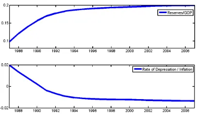
in-flation and exchange rate depreciation are the mirror image of international

reserves. As the stock of international reserves increases, inflation is ever smaller and exchange rate depreciation decreases. If a crisis hits, the central

banks uses a mix of inflation and reserves to finance the deficit. The larger

the reserve holdings at the moment of the crisis, the smaller is the increase in inflation.

Second, I perform some experiments that highlight the sources of variation

(45)

reserves accumulation in my model. The more elastic is capital relative to consumption, the larger is the buffer stock of international reserves.

Fur-thermore, I investigate the effect of the frequency of crises and constraints

on borrowing by the central bank. The frequency of crises is not a crucial determinant of the buffer stock. This is intuitive. If a crisis hit every period,

then crises were already smooth and there is no role for reserve policy.

Re-serves are most useful when crises are rare and large. Borrowing constraints, however, play an important role. A central bank that is able to borrow 10%

ofGDP, instead of the 0% I use as a baseline, sees a reduction in its buffer

stock of international reserves of almost one half.

1.4.1 An average developing economy

Parameter values

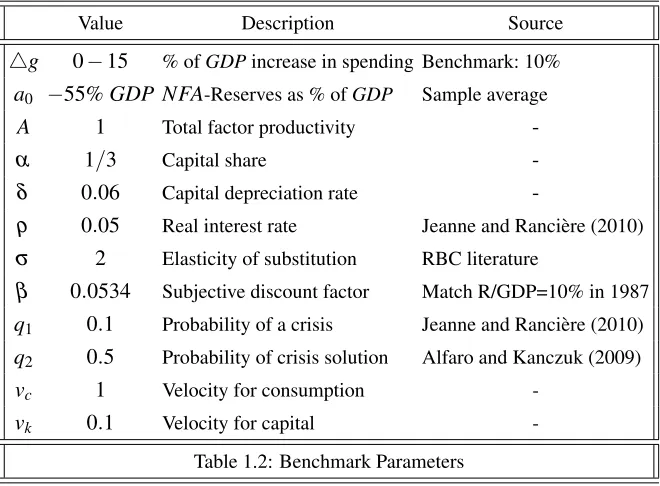
In Table 1.2 I report values for the parameters used in the baseline case.26

The parameters for the real interest rateρ and the probability of a crisis

q1 come from Jeanne and Ranci`ere (2010). The parameter governing the

probabilistic end of the crisisq2is taken from Alfaro and Kanczuk (2009).

Together, they mean that a crisis happens on average once every 10 years and lasts on average 2 years.27 To calibrate the production function I use

traditional values for the share of capitalα=1₃ and for the depreciation rate

δ=0.06. I setA=1.

Two crucial parameters are the financing needs in the low and in the high

spending states. I normalizegL=0, and do the analysis for values ofgH

between 5 and 15% ofGDP. Table 1.2 presents available evidence of the fiscal costs of bailing out the banking system in developing economies. The

relevant cost for this exercise is the amount accruing to the central bank,

26_{Throughout, crises are computed as a share of potential output. This means that crises}

are measured in absolute terms. Reserves are measured with respect to current output, are measured in relative terms.

27_{Although these parameters capture the incidence of sudden stops, banking crises and}

(46)

that needs to be financed with inflation related revenues. Burnside et al (2006) perform 3 case studies: Korea 1997-2002, Mexico 1994-2002 and

Turkey 2001-2002. They find that in these three episodes total

inflation-related financing up to 2002 was in present value around 20% of pre-crisis

GDP.28

Value Description Source

4g 0−15 % ofGDPincrease in spending Benchmark: 10%

a₀ −55%GDP NFA-Reserves as % ofGDP Sample average

A 1 Total factor productivity

-α 1/3 Capital share

-δ 0.06 Capital depreciation rate

-ρ 0.05 Real interest rate Jeanne and Ranci`ere (2010)

σ 2 Elasticity of substitution RBC literature

β 0.0534 Subjective discount factor Match R/GDP=10% in 1987

q1 0.1 Probability of a crisis Jeanne and Ranci`ere (2010)

q2 0.5 Probability of crisis solution Alfaro and Kanczuk (2009)

vc 1 Velocity for consumption

-vk 0.1 Velocity for capital

-Table 1.2: Benchmark Parameters

How do these costs compare to previous work on international reserves? Previous literature has focused on output shocks and sudden stops of capital

inflows. Jeanne and Ranci`ere (2010) assume that a representative agent

loses access to foreign debt of 10% ofGDPand suffers an output loss of 6.5% of trendGDP. Alfaro and Kanczuk (2009) assume an output loss of

28_{It is important to note that Burnside et al (2006) argue that, at least for the cases of Korea,}

[image:46.499.86.416.189.432.2]

(47)

10% during a default crisis. In my setup,gcan be directly interpreted as an output shock that hits part of the economy (the central bank).

Some parameters are not taken from previous work. I normalizevc=1 and

choose vk =0.1. These parameters will guide the relative importance of

distortions. They capture unobserved features of the economy that

deter-mine how distortionary is inflation. For example, adjustment costs to capital can be captured by this parametervk. I perform a sensitivity analysis on

these parameters in Section 4.2. The borrowing constraint is assumed to be

r=0% ofGDP. That is, I assume that the central bank can not access swap

lines with other central banks or any type of debt financing.

Country Date of Estimate Fiscal cost of Increase in Inflation

banking crises Public debt financed

Indonesia Nov. 99 65 -

-Korea Dec. 99 24 - 22.3

Malaysia Dec. 99 22 -

-Mexico Nov. 94 15 - 24

Thailand Jun. 99 35 -

-Turkey Jan. 01 18 - 19.2

Developing* 1970-2006 11.5 12.7 -Developed* 1970-2006 3.7 36.2

-Table 1.3: Burnside et al (2001), (2006),present value, % of pre-crisis GDP.

* Laeven and Valencia (2010), cumulative, % of current GDP.

Finally, I choose a free parameter in the model, the discount rate β to

match the buffer stock of _GDPRES =10% in 1987 as the long-run buffer stock in a world where a crisis is given bygH,0 =6% of GDP. This number

is obtained by comparing the size of the financial sector in the developing

world, as measured byM2/GDP, with its 2007 counterpart:M2/GDP1987≈ 3

[image:47.499.95.407.283.484.2]

(48)

Baseline Results

Table 1.4 collects the results of the benchmark calibration. As argued above,

I consider as a baseline an increase in spending given by4gt =10%. The

level of international reserves in the long-run predicted by the model is 20.66% ofGDP. Remember that this value corresponds to the level of

in-ternational reserves obtained as the outcome of optimal policy following a

long period without a crisis.

4gt Long run reserves

0.05 8.50% 0.1 20.66%

[image:48.499.178.320.239.335.2]

0.15 33.11%

Table 1.4:RES/GDP(r=0%)

Figures 1.8 and 1.9 show the path of reserves and exchange rate depreciation

before and after a crisis. In Figure 1.8 it is possible to see that in the absence of a crisis, 20 years suffices to approach the long-run buffer stock of

re-serves. The way accumulation is done is through a decreasing inflation rate,

which translates into a depreciating exchange rate. Figure 1.9 shows the ef-fect of a crisis on reserves and exchange rates. Note how when reserves are

larger, in the first crisis, exchange rate depreciation is smaller. Obstfeld et al

(2009) shows that countries with larger international reserve holdings deval-ued (and in some cases even appreciated) their currencies less. Dominguez

et al (2011) shows that countries drew from international reserves and al-lowed for some currency depreciation following the 2008 financial crisis.

What kept exchange rates from depreciating further was the use of reserves.

(49)

[image:49.499.149.352.76.198.2]

Figure 1.8: Reserves and exchange rate depreciation on the reserve accu-mulation path.

Figure 1.9: Reserves and exchange rates during two crises.

Before investigating the sources of variation behind the long-run level of reserves, I perform a sensitivity analysis on the risk-aversion parameter. As

will be clear in Section 1.4.3, this is useful to compare with the consumption

smoothing perspective. Table 1.5 collects the results. As expected, larger risk aversion increases the long run level of reserves.

σ Long run reserves

1 17.71% 2 20.66%

3 24.50%

Table 1.5:RES/GDP(r=0%),4gt

[image:49.499.153.343.533.629.2]

(50)

1.4.2 Sources of variation

This section explores the determinants of the stock of international reserves suggested by the model. I highlight the role of distortions, the relative

im-portance of the frequency and magnitude of a crisis, and the effect of

bor-rowing constraints. To study the impact of distortions on reserves, I perform an analysis varying the two velocity parametersvcandvk. These parameters

measure the relative importance of the different distortions in the economy,

that is, they determine how large the elasticity of savings and capital is rela-tive to the interest rate. Ifvc=0, the only distortion is on the capital stock.

In this open economy setting with free capital movements, the capital stock

can be adjusted without any cost and is therefore very elastic to changes in the domestic interest rate. Distortions are large. As a consequence, the

buffer stock of reserves is also large. If vk =0, inflation does not have

an impact on output and distortions are relatively small. This is because

consumption is less elastic than production. Table 1.6 shows the result of

changing these two parameters.

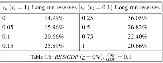
vk (vc=1) Long run reserves vc(vk=0.1) Long run reserves

0 14.99% 0.25 36.05%

0.05 15.96% 0.5 26.82% 0.1 20.66% 0.75 22.40%

[image:50.499.106.392.383.495.2]

0.15 25.89% 1 20.66%

Table 1.6:RES/GDP(r=0%),4gt

GDP=0.1

This analysis shows that what is important is the relative size of the two ve-locity parameters. If one of the velocities is zero, different values ofvjust

have an impact on the level of inflation but not on the distortions. We can

see that reserves increase the most when production distortions are more im-portant. This suggests that consumption/savings distortions should be less

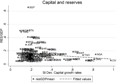
associated with reserves than production distortions. Figure 1.10 and 1.11

(51)

standard deviation of capital and consumption growth rates over the period 1987-2007. Reserves are inversely related with the standard deviation of the

growth rate of the capital stock, but are not related to consumption growth.

That is, larger average international reserves between this period are asso-ciated with lower volatile growth rates in capital, but not in consumption.

This showcases the importance of the capital distortion in the international

[image:51.499.133.372.201.371.2]

reserves accumulation process.29

Figure 1.10: Average reserves to GDP ratio and standard deviation of cap-ital growth rates over 1987-2007 for developing economies. Source: Own calculations from the PWT - Heston et al (2011) and Lane & Milesi-Ferretti (2010). The slope is negative and significant at the 5% level.

The analysis so far has considered large and infrequent crisis. How do these compare with costlier but less frequent crises? The first panel of Table 1.7

collects the level of reserves in that case. Consider instead that a country

faces an undisciplined fiscal authority, constantly demanding financing with the central bank, and spending crises are small but frequent. The second

panel of Table 1.7 collects the buffer stock of reserves in that case.

Compar-ing the numbers, it is possible to see that the crucial dimension to explain the growth of reserves is the existence of large and infrequent crises.

29_{Figures 1.10 and 1.11 plots all the data. Removing the outliers in both figures, only}

(52)

[image:52.499.134.374.76.245.2]

Figure 1.11: Average reserves to GDP ratio and standard deviation of con-sumption growth rates over 1987-2007 for developing economies. Source: Own calculations from the PWT - Heston et al (2011) and Lane & Milesi-Ferretti (2010).

q₁

4gt

GDP=0.15

Buffer Stock q₁

4gt

GDP=0.05

Buffer Stock

0.025 25.27% 0.15 8.75%

0.05 32.34% 0.2 8.93% 0.075 32.81% 0.3 9.00%

Table 1.7:RES/GDP(r=0%)

I now investigate the effect of the borrowing constraint faced by the

cen-tral bank. This was a crucial determinant of reserves in the deterministic example. The ability to borrow in the event of a crisis is also an

impor-tant difference between developed and developing economies. In the 2008

crisis, some central banks established swap lines between them, to ensure liquidity of foreign currency in a period of distress. Central banks in

devel-oping economies could not access these credit lines (Obstfeld et al 2009).

[image:52.499.104.397.337.435.2]

(53)

ras % ofGDP Buffer Stock

+15% 38.62%

+10% 28.51%

0% 20.66%

−10% 11.50%

−15% 4.10%

Table 1.8:RES/GDP, 4gt

GDP=0.1

To sum up, the quantitative analysis of the model shows that reserves ad-equacy should be measured with respect to the magnitude of the financing

needs, the distortions caused by inflation and the ability to access

contin-gent financing following a crisis. In particular, the capital distortion seems to play a crucial role in the determination of reserve stocks.

1.4.3 Comparison with consumption smoothing

To make the role of distortionary inflation smoothing clear I solve for a model where distortions are not important. It is possible to show that the

consumption smoothing view is a particular case of the inflation smoothing

perspective even if inflation is the only tax possible. This is the case if in-flation does not distort output and if the elasticity of savings to the interest

rate is zero. These are precisely the two sources of distortions described in

section 3. Intuitively, if the consumer always allocates the same share of wealth to consumption services every period, and this wealth is unaffected

by monetary policy, inflation is non-distortionary. For the purposes of

re-serve accumulation, the economy is sufficiently well described by a single agent performing consumption smoothing. As an implication, it follows that

these two features - that inflation affects output and savings - are crucial for

the quantitative predictions of the model.30

I perform the same quantitative experiment for the consumption smoothing

model in the baseline parametrization withgH=10% of GDP. The long

30_{Appendix A.3 shows that if}_a·₌_{0 and}_v