Global instability in the elliptic restricted three body problem

(1)

Global instability in the elliptic restricted three body

problem

Thesis presented to obtain the Ph. D. in Applied Mathematics by

Universitat Polit`ecnica de Catalunya

Abraham De la Rosa Ibarra

Supervisors: Tere M. Seara and Amadeu Delshams

(2)

Acknowledgements

I would like to express my deep gratitude to Professors Tere M. Seara and Amadeu Delshams, my research supervisors, for their patient guidance, encouragement and support during all the process my Ph. D. needed, I am very grateful.

To every member of the examination panel I want to express my gratitude, Professors: Carles Simò, Marian Gidea, Regina Mart´ınez, Pau Martin, Marcel Guàrdia, Imma Baldomà and Ernest Fontich.

I would also like to thank all Professors that form the Dynamical Systems Group of the UPC and extend my thanks to Professors at UB, altogether, have contributed to my formation as well as other young researchers, that have become my friends. Thank you Marina for helping me when I needed.

My sincere gratitude to all the administrative staff of the Department of Applied Mathematics I, thank you Ester and Hilda. Also, at the faculty of Mathematics and Statistics, thank you Raquel and Carme, for your patience and help during all these years.

I am grateful with the UPC for the grant “FPI-UPC Recerca” that was given to me, it made possible for me to do the Ph. D.

(4)

Introduction

Celestial mechanics has been a continuous source of inspiration of the main problems arising in dynamical systems. Particularly, the phenomenon of chaos and the existence of homoclinic orbits appears for the first time in the memory of Poincar´e about the stability of the three body problem [Hen90], where the first exponentially small splitting of separatrices was computed.

In this memory we deal with the elliptic restricted three body problem (ERTBP) which appears in a natural way to study global instability, since it has two and a half degrees of freedom. The global instability, commonly known as diffusion, or better said, Arnold diffusion, from the pioneer work of Arnold in 1964 [Arn64], has been studied in the ERTBP in several settings, or more precisely, in several zones of the phase space. Capinsky & Zgliczynski have studied the instability in this problem, close to librations points in [CZ11] following previous work of Llibre & Simó [LS80b] and Llibre, Martinez & Simó [LMS85] for the existence of transversal homoclinic orbits in the classical circular restricted three body problem (CRTBP), as well as Bolotin close to collision [Bol06], Xia has studied micro-diffusion in the ERTBP [Xia93]. Recently, diffusion along mean motion resonances in the ERTBP model for Sun-Jupiter-asteroid systems has been proven by Fejoz, Guardia, Kaloshin & Roldán in [FGKR14]

In the last years, there have bee several mechanisms used to prove diffusion, like variational and geometrical methods. This memory is based on the application of geometrical methods, which are based on the existence of a scattering map associated to a normally hyperbolic invariant manifold (NHIM) in the phase space [DdlLS08, DGdlLS08]. In such cases, both the inner dynamics inside the NHIM as well as the outer dynamics provided by the scattering map, are combined to design diffusing pseudo-trajectories, consisting on invariant tori plus their transversal heteroclinic connections, that is, transition chains in Arnold’s language.

In this memory we deal with the existence of diffusion orbits of the ERTBP whose angular momentum increases. Those orbits correspond to motions where the comet moves far from the primaries and comes back many times, increasing at each turn its angular momentum by a small amount.

The ERTBP is a Hamiltonian system of two and a half degrees of freedom. The so-called manifold of infinity can be seen, after a suitable change of variables provided by McGehee in [McG73], as a three dimensional invariant manifold in the extended phase space which behaves topologically as a NHIM, although it is of parabolic type. This means that the rate of approach and departure from it along its invariant manifolds is polynomial in time, instead of exponential-like as happens in a standard NHIM. On the other hand, the inner dynamics is very simple, since it is formed by a two-parameter family of 2π-periodic orbits in the 5D extended phase space which correspond to constant solutions in the 4D phase space. As a consequence, the stable and unstable manifold of the infinity manifold are union of the stable and unstable manifolds of its periodic orbits, and as long as these manifolds intersect along transversal heteroclinic orbits, the scattering map can be defined. Unfortunately, since the inner dynamics of the infinity manifold is so simple, the classical mechanisms of diffusion, consisting of combining the inner and outer dynamics, do not work here. Instead, as a novelty, we will be able to find two different scattering maps which will be combined in a suitable way to provide orbits whose angular momentum increases.

(5)

which was later corrected and carried out formally for the ERTBP in [MP94]. In both works, one can realize the massive amount of computations required.

In Chapter 2 of this memory, we provide a rigorous computation of the so-called Melnikov potential, with asymptotics and rigorous bounds for the errors for some range of the parameters

µ(mass parameter),e0 (eccentricity of the primaries) andG0 (angular momentum of the comet). More precisely, the results presented here, are valid forG0big enough,e0G0bounded andµsmall enough.

In Chapter 1, the problem is introduced, as well as the main geometrical objects which play a role in the diffusion mechanism. Particularly, the infinity manifold, its stable and unstable manifolds and the two independent scattering maps as well as the asymptotic formulas for them. The combination of both of them lead to theorem 1.15 fore0G0 =λsmall, and theorem 1.16 for

e0G0=λfinite, at the end of the chapter.

(6)

Chapter 1

Main results

1.1 Preliminars

As in the classical setting of the restricted three body problem, consider a particle with zero mass that moves in the plane generated by the dynamics of two point masses calledprimaries. It is a well known fact that the primaries move over an ellipse with a focus in the center of mass and with certain eccentricity that we will call e0. If we fix a coordinate reference system with the origin at the center of mass and call q1 and q2 the position of the primaries, then under the classical assumptions regarding time units, distance and masses normalization, the motion of the third particle whose position we will callqis given by

d2_q

dt2 =

(1−µ)(q1(t, e0)−q)

|q1(t, e0)₋q_|3 +

µ(q2(t, e0)−q)

|q2(t, e0)₋q_|3 (1.1) where 1−µis the mass of the particle atq1 andµthe mass of the particle atq2. If we introduce the conjugate momentap=dq/dtand the self-potential function (see [MHO09, p. 28])

Uµ(q, t;e0) =

1₋µ

|q−q1(t, e0)|+

µ

|q−q2(t, e0)| (1.2)

This equation can be rewritten as a Hamiltonian system with Hamiltonian

Hµ(q, p, t;e0) =

p2

2 −Uµ(q, t;e0). (1.3) This is a time-periodic Hamiltonian of two and a half degrees of freedom.

By the first Kepler law the distance between the primaries (see [Win41, p. 194-195]) is given by

r0(t) = 1−e 2 0 1 +e0cosf

(1.4)

wheref is the so calledtrue anomaly (see [Win41, p. 203], [MP94, p. 303]), which satisfies

df dt =

(1 +e0cosf)2 (1₋e2

0)3/2

. (1.5)

or also by

r0(t) = 1₋e0cosE (1.6) in terms of theeccentric anomaly E, given by the Kepler equation (see [Win41, p. 195])

(7)

1.2 Changes of coordinates and setting of the problem

Because of the nature of the problem we are dealing with, it will be better to perform a polar-simplectic change of variables, to the Hamiltonian (1.3) say

X =rcosα (1.8a)

Y =rsinα (1.8b)

whereq= (X, Y). Now, we look for conjugate momentaPrandPαso that the change

(X, Y, PX, PY) ϕ

−→ (r, α, Pr, Pα) (1.9)

is canonical. Following [Gol65], we get:

PX=Prcosα−

Pα

r sinα (1.10a)

PY =Prsinα−

Pα

r cosα. (1.10b)

In this way, the change of variables (1.10) is simplectic and the equations of motion in the new coordinates are the associated to the Hamiltonian

H∗

µ=Hµ(ϕ(Q), t;e0)

that we will write as

Hµ∗(r, α, Pr, Pα, t;e0) =P

2

r

2 +

P2

α

2r2 −Uµ∗(r, α, t;e0) (1.11)

andU∗

µ defined by

Uµ∗(r, α, t;e0) =Uµ(rcosα, rsinα, t;e0). (1.12)

In this notation, the primaries are

q2=q2(t, e0) =−rJ(t, e0)(cosf(t, e0),sinf(t, e0)) (1.13a)

q1=q1(t, e0) = rS(t, e0)(cosf(t, e0),sinf(t, e0)). (1.13b)

where

rJ(t, e0) = (1−µ)r0(t), rS(t, e0) =µr0(t)

and

|q−q2|2 =r2+ 2(1−µ)r0(t)rcos(α−f) + (1−µ)2[r0(t)]2,

|q−q1|2 =r2− 2µ[r0(t)]rcos(α−f) +µ2[r0(t)]2. From now on we will write

G=Pα, y =Pr.

and then Hamiltonian (1.11) reads

Hµ∗(r, α, y, G, t;e0) =

y2 2 +

G2

2r2 −Uµ∗(r, α, t;e0)

withU∗

(8)

1.2.1 McGehee coordinates

To study the behavior of orbits near infinity, we make to the Hamiltonian equations of Hamiltonian

H∗

µ(r, α, y, G, t;e0) the non-canonical change of variables:

r= 2

x2 (1.14)

to we get the so calledMcGehee coordinates (see [MP94] y [McG73]). Defining

Uµ(x, α, t;e0) =Uµ∗(2/x2, α, t;e0) (1.15)

the equations associated to (1.11) become: ˙

x=−1₄x3y y˙ =1 8G

2_x6

−x

3 4

∂Uµ

∂x (1.16a)

˙

α= 1 4x

4_G _G_˙ ₌∂Uµ

∂α (1.16b)

where

Uµ(x, α, t;e0) =

x2 2

₁ −µ σ1 +

µ σ2

(1.17) and

σ2

1 = 1−z1x2cos(α−f) + 1 4z

2

1x4, z1=µr0(t),

σ2

2 = 1 +z2x2cos(α−f) + 1 4z

2

2x4, z2= (1−µ)r0(t),

It is important to notice that f is present in these equations, and then, becomes necessary to add the equation for f given in (1.5) in order to have the complete description of the dynamics. Equations (1.16) were obtained in [MP94].

Hamiltonian structure

Proposition 1.1(quasi-Hamiltonian structure). IfHµ is defined by

Hµ(x, α, y, G, t;e0) =

y2 2 +

x4_G2

8 − Uµ(x, α, t;e0), (1.18) and_U is given in (1.17), the equations (1.16) can be written as

˙

x=₋x 3 4

∂_Hµ

∂y

˙

y=₋x 3 4

−∂_∂xHµ

(1.19a)

˙

α= ∂Hµ

∂G G˙ =−

∂Hµ

∂α (1.19b)

Therefore, equations (1.19) are in fact Hamiltonian with symplectic (non-canonical) form as-sociated:

ω(z)(u,v) =uT_J−Tv (1.20) where_J =J_Dwith_D= diag(₋x3_/₄_,₁_,

−x3_/₄_,_{1) and}_J _{the symplectic matrix}

J =

0 I2

−I2 0

.

As in the classical theory we can write equations (1.19) in terms of the Poisson bracket

{{f, g}}(z) =∇f(z)TJ ∇g(z) =₋x

3 4

∂f ∂x

∂g ∂y−

∂f ∂y

∂g ∂x

!

+∂f

∂α ∂g ∂G−

∂f ∂G

∂G

(9)

1.3 Invariant manifolds

In order to analyze the structure of system (1.19), we will write_Hµ given in (1.18) as

Hµ(x, α, y, G, t;e0) =H0(x, y, G) +µUµ∗(x, α, t;e0) (1.22)

or equivalently we write_Uµ in (1.18) as

Uµ(x, α, t;e0) =U0(x) +µUµ∗(x, α, t;e0) =

x2 2 +µU

∗

µ(x, α, t;e0) (1.23)

and then study the dynamics as a perturbation of the limit caseµ= 0. From (1.23),

U∗

0(x, α, t;e0) = lim

µ→0 1

µ

Uµ(x, α, t;e0)−

x2 2

= x

2

4 +x4_r2

0+ 4x2r0cos(α−f) 1/2 +

_x2 2

2

r0cos(α−f)−

x2

2 (1.24)

1.3.1 The limit case

µ

= 0

In this case, the Hamiltonian given in (1.18) becomes

H0(x, α, y, G) =y 2 2 +

x4_G2

8 − U0(x) =y

2 2 +

x4_G2 8 −

x2

2 (1.25)

As the system is autonomous_H0is a first integral. Moreover,H0 is independent ofe0 andα. The equations associated to Hamiltonian (1.25) are

˙

x=₋1 4x

3_y _y_˙₌ 1

8G 2_x6

−1₄x4 _(1.26a) ˙

α= 1 4x

4_G _G_˙ _{= 0} _(1.26b)

where it is clear thatGis a conserved quantity.

The level curves of_H0 are represented in Figure 1.1 forGfixed andH0=h.

x y

h= 0

h >0

[image:9.595.89.206.529.713.2]

h <0

Figure 1.1: Level curves of_H0

First, the phase space is given by (x, α, y, G)∈R_×T_×R2_.

From equations (1.26) it is clear that

E =_{z= (x, α, y, G)_∈R_×T_×R_×R_+; _x_{= 0}_} _(1.27)

is the set of equilibrium points of the system. Moreover, for any fixedα0∈T, G0∈R,

Λα0,G0={(0, α0,0, G0)}

is a parabolic critical point with stable and unstable 1-dimensional invariant manifolds:

γα0,G0 = W

u_(Λ

α0,G0) =W

s_(Λ α0,G0) =

z= (x, α0, y, G0), H0(x, y, G0) = 0, α=α0−G0

Z

H0=0

x ydx

(10)

In a natural way, we define the 2-dimensional manifold Λ∞=

[

α0,G0

Λα0,G0,

which is a “normally parabolic” invariant manifold with stable and unstable 3-dimensional invariant manifolds

γ=Wu(Λ∞) =Ws(Λ∞)

=_{z= (x, α, y, G), _H0(x, y, G) = 0_}.

As we will deal with a periodic in time Hamiltonian, let us work in the extended phase space ˜

z= (z, s) = (x, α, y, G, s)_∈R_×T_×R2_×T

just by adding the equation ˙s= 1 to the systems (1.19) and (1.26). Now we are going to write the extended version of the invariant sets we have defined so far. For anyα0∈T, G0∈R, the set

˜

Λα0,G0 ={z˜= (0, α0,0, G0, s0), s0∈T} (1.28) is a 2π-periodic orbit with motion determined by ˙s= 1.

The manifold ˜

γα0,G0 =W

u_(˜_Λ

α0,G0) =W

s_(˜_Λ α0,G0) =

z= (x, α0, y, G0, s0), s0∈T, H0(x, y, G0) = 0, α=α0−G0

Z

H0=0

x ydx

.

is a 2-dimensional homoclinic manifold to the periodic orbit ˜Λα0,G0. On the other hand we can construct the 3-dimensional invariant manifold

˜ Λ∞=

[

α0,G0 ˜

Λα0,G0 ={(0, α0,0, G0, s0),(α0, G0, s0)∈T×R×T}. (1.29)

As the motion for points in ˜Λ∞is given by the dynamics on each ˜Λα0,G0, taking ˜

x0= ˜x0(α0, G0, s0) = (0, α0,0, G0, s0)∈Λ˜∞≃R×T2

the inner dynamics on ˜Λ_∞(see [DdlLS06]) is trivial: ˜

φt,0(˜x0) = (0, α0,0, G0, s0+t) = ˜x0(α0, G0, s0+t)∈Λ˜∞. (1.30)

The 4-dimensional stable and unstable manifolds of ˜Λ_∞ coincide along the 4-dimensional ho-moclinic invariant manifold

˜

γ = Wu(˜Λ∞) =Ws(˜Λ∞)

= _{(x, α, y, G, s),(α, G, s)_∈T_×R_×T_, _H₀₍_{x, α, y, G}_{) = 0}_} _(1.31)

It is possible to parameterize ˜γα0,G0 by the solutions of the Hamiltonian flow contained in

H0= 0 in some timeτ satisfying (see [MP94] )

dt dτ =

2G x2.

So that, the homoclinic solution to the periodic orbit ˜Λα0,G0 of the system (1.26) can be written as

xh(t;G0) = ˜xh(τ;G0) (1.32a)

(11)

yh(t;G0) = ˜yh(τ;G0) (1.32c)

Gh(t;G0) =G0 (1.32d) whereα0 andG0are free parameters and the relation

t= G 3 0 2

τ+τ 3 3

(1.33) holds. The equations (1.32) are explicitly, inτ-time, given by

˜

xh(τ;G0) =

2

G0(1 +τ2₎1/2, α˜h(τ) = 2 arctan(τ), y˜h(τ;G0) = 2τ

G0(1 +τ2₎. (1.34) With this in mind, we have that taking

˜

z0=˜z0(ν, α0, G0, s0) = (z0(ν, α0, G0), s0)

= (xh(ν;G0), αh(ν;α0, G0), yh(ν;G0), G0, s0)∈˜γ (1.35) we can write

˜

γα0,G0 ={˜z0= (xh(ν;G0), αh(ν;α0, G0), yh(ν;G0), G0, s0), ν∈R, s0∈T}. Finally ˜γ can be seen as a union of homoclinic orbits to ˜Λ_∞(homoclinic manifold).

˜

γ= [

α0,G0 ˜

γα0,G0

and then we can parameterize the 4-dimensional homoclinic manifold as ˜

γ=W(˜Λ_∞) =_{(xh(ν;G0), αh(ν;α0, G0), yh(ν;G0), G0, s0), ν ∈R, G0∈R,(α0, s0)∈T2}. (1.36) and the motion in ˜γ is given by

˜

φt,0(˜z0) = (xh(ν+t;G0), αh(ν+t;α0, G0), yh(ν+t;G0), G0, s0+t)∈˜γ.

1.3.2 The case

µ

₆

= 0

In the general case, we should note some things regarding the manifolds defined in section 1.3.1. First of all the set_Eremains invariant and, therefore, so does ˜Λ_∞, being again a “normally parabolic invariant manifold”, and the periodic orbits ˜Λα0,G0 persist. The inner dynamics on ˜Λ∞, that is the flow restricted to it is also trivial

(α0, G0, s0)→(α0, G0, s0+t). (1.37)

1.4 Melnikov potential for the parabolic orbits

From [McG73] we know thatWs

µ(˜Λ∞) andWµu(˜Λ∞) exist forµsmall enough and are 4-dimensional

in the extended space. The classical geometric Melnikov method to find the first order approxima-tion to the distance between the perturbed manifolds will work in this case because both manifolds have co-dimension one, and then, a normal vector to ˜γwill intersectWu

µ(˜Λ∞) andWµs(˜Λ∞) forµ

small enough.

Let us take˜z0= (z0, s0) = (z0(ν, α0, G0), s0)∈γ˜as in (1.35). Now, we have to construct points inWs

µ(˜Λ∞) andWµu(˜Λ∞) to measure the distance between them. It is clear from the definition of

˜

γthat

(12)

is orthogonal to ˜γ=Wu(˜Λ∞) =Ws(˜Λ∞) and then if the normal bundle is defined by

N(˜z0) =_{˜z0+σv, σ∈R} we have that there exist unique points˜zu,s_µ = (zu,s

µ , s0) such that

{˜zu,s_µ _}=Wµu,s(˜Λ∞) ∩N(˜z0). (1.38)

The distance we want to compute is the signed magnitude given by

d(˜z0, µ) =_H0(˜z_µu)_{− H}0(˜zs_µ). (1.39) Define (see [DdlLS06])

L(α0, G0, t0;e0) =

Z ∞ −∞U

∗

0(xh(s;G0), αh(s;α0, G0), s+t0;e0)ds (1.40) which is a convergent integral because of formulas (1.32)-(1.34), and

U∗

0(x, α, s;e0) =O(x2) as x→ ∞

Proposition 1.2. Given (α0, G0, s0)∈T×R+×Tassume that the function

ν_∈R_{−→ L}₍_α₀_{, G}₀_{, s}₀₋_ν_;_e₀₎_∈R _(1.41)

has a non-degenerate critical pointν∗ ₌ _ν∗₍_α

0, G0, s0;e0). Then for 0 < µ small enough, there exists a locally unique point

˜

z∗=˜z∗(ν∗, α0, G0, s0;µ)∈Wµs(˜Λ∞)⋔Wµu(˜Λ∞)

of the form

˜z∗=˜z∗₀+O(µ) where ˜z∗

0 = (xh(ν∗;G0), αh(ν∗;α0, G0), yh(ν∗;G0), G0, s0) ∈ ˜γ. Also, there exist unique points ˜z_±= (0, α_±,0, G_±, s0) = (0, α0,0, G0, s0) +O(µ)∈Λ˜∞ such that

φt,µ(˜z∗)−φt,µ(˜z±)→0 fort→ ±∞ (1.42)

Then, we have

G+−G−=µ

∂_L ∂α0

(α0, G0, s0−ν∗(α0, G0, s0)) +O(µ2).

Proof. From equation (1.35) we know that any point˜z0∈γ˜ have the form ˜

z0=˜z0(ν, α0, G0, s0). As we have seen in (1.38)

˜

z_µu,s= (˜zu,sµ , s0)∈Wµu,s(˜Λ∞)∩N(˜z0).

We are looking for˜z0 such that ˜zs_µ=˜zu_µ. From this, there must exist points˜z_± = (˜z±, s0)∈Λ˜∞

such that

φt,µ(˜zs,uµ )−φt,µ(˜z±)−−−−→_t

→±∞ 0, (1.43)

moreoverφt,µ(˜zs,uµ )−φt,0(˜z0) = O(µ) (see [McG73]). Since H0 does not depend on time, by the chain rule we have that

d

dtH0(φt,µ(˜z

s,u

(13)

SinceH0= 0 in ˜Λ∞, using (1.43) and the trivial dynamics on ˜Λ∞we obtain

H0(˜zs,u_µ ) =−µ

Z _±∞

0 {{H

0,Uµ∗}}(φs,µ(˜zs,uµ ))ds.

Finally, using Taylor’s series inµ,

H0(˜zu_µ)− H0(˜zs_µ) =µ

Z ∞ −∞{{H

0,U0∗}}(φt,0(˜z0))dt+O(µ2)

=µ

Z ∞ −∞{{H

0,U0∗}}(xh(ν+t;G0), αh(ν+t;α0, G0), yh(ν+t;G0), G0, s0+t)dt+O(µ2) On the other hand, from (1.40),

L(α0, G0, t0;e0) =

Z ∞ −∞U

∗

0(xh(s−t0;G0), αh(s−t0;α0, G0), s;e0)ds and then

∂L

∂t0

(α0, G0, t0;e0) =−

Z _∞

−∞{{U ∗

0,H0}}(xh(s−t0;G0), αh(s−t0;α0, G0), yh(s−t0;G0), G0, s)ds =

Z ∞ −∞{{H

0,U0∗}}(xh(s−t0;G0), αh(s−t0;α0, G0), yh(s−t0;G0), G0, s)ds so that

∂_L ∂t0

(α0, G0, s0−ν;e0) =

Z ∞ −∞{{H

0,U0∗}}(xh(s−s0+ν;G0), αh(s−s0+ν;α0, G0), yh(s−s0+ν;G0), G0, s)ds =

Z ∞ −∞{{H

0,U0∗}}(xh(t+ν;G0), αh(t+ν;α0, G0), yh(t+ν;G0), G0, s0+t)dt and therefore

d(˜z0, µ) =H0(˜zuµ)− H0(˜zsµ) =µ

∂L

∂t0(α0, G0, s0−ν;e0) +O(µ 2₎

Now, it is clear by the implicit function theorem, forµsmall enough, that a non degenerate critical valueν∗_{of the function (1.41) gives rise to homoclinic points to ˜}_Λ

∞where the manifoldsWµs(˜Λ∞)

andWu

µ(˜Λ∞) intersect transversally that have the desired form˜z∗=˜z∗0+O(µ).

Consider now the solution of the system (1.19) represented by φt,µ(˜z∗). Moreover, by the

fundamental theorem of calculus and the definition (1.18) we have

G+−G− =−

Z ∞ −∞

∂_Hµ

∂α (φt,µ(˜z

∗₎₎_dt₌Z ∞ −∞

∂_Uµ

∂α (φt,µ(˜z

∗₎₎_dt

=µ

Z ∞ −∞

∂U∗

0

∂α (φt,0(˜z

∗

0))dt+O(µ2) =µ

Z ∞ −∞

∂_U∗

0

∂α (xh(ν

∗₊_t_;_G₀₎_{, α}

h(ν∗+t;α0, G0), yh(ν∗+t;G0), G0, s0+t)dt+O(µ2) =µ∂L

∂α(α0, G0, s0−ν

∗_;_e_{0) +}_O₍_µ2₎_.

Once we have found a critical pointν∗ _{of (1.41) we define the reduced Poincar´e function (see}

[DdlLS06])

L∗₍_α

(14)

The scattering map

The scattering mapS is defined from the manifold ˜Λ_∞(defined in (1.29)) to itself. Take˜z₋,˜z+∈ ˜

Λ_∞, then

Sµ(˜z−) =˜z+

if there exist˜z∗_∈Wu

µ(˜Λ∞)⋔Wµs(˜Λ∞) such that

φt,µ(˜z∗)−φt,µ(˜z±)→0 fort→ ±∞. (1.45)

In the caseµ= 0 we have that ˜γ=Wu_(˜_Λ

∞) =Ws(˜Λ∞) implies that the scattering mapS0is the identity. Indeed, for a generic point

˜

x0= (0, α0,0, G0, s0)∈Λ˜∞

we haveS0(˜x0) = ˜x0. To see this, take

˜z0= (xh(ν;G0), αh(ν;α0), yh(ν;G0), G0, s0)∈γ˜ then by equations (1.32), (1.33) and (1.34)

φt,0(˜z0)−φt,0(˜x0) =

(xh(t+ν;G0), αh(t+ν;α0), yh(t+ν;G0), G0, t+s0)−(0, α0,0, G0, t+s0)−−−−→

t→±∞ 0

wich proves thatS0=Id.

The next proposition gives an approximation of the scattering map in the general caseµ₆= 0 Proposition 1.3. The scattering mapSµ associated to the non degenerate critical pointν∗of the

function defined in (1.41) is given by (0, α₋,0, G₋, s₋)_7−→0, α₋+µ∂L∗

∂G(α−, G−;e0) +O(µ

2₎_,₀_{, G}

−−µ

∂_L∗

∂α (α−, G−;e0) +O(µ

2₎_{, s}

−

where_L∗ _{is the Poincar´e reduced function introduced in (1.44).}

Proof. By hypothesis we have a non degenerate critical point ν∗ _{of (1.41), by using definition}

(1.44) the proposition 1.2 gives the correspondence we look for betweenG− andG+. Finally, the

equation

α+−α− =−µ

∂_L∗

∂G(α0, G0, t

∗

0) +O(µ2)

is a direct consequence of the fact that_L∗ _{is symplectic, as shown in [DdlLS08].}

Since we know that for all time,

φt,µ(˜z∗) =φt,0(˜z∗0) +O(µ),

denotingG(φt,µ(˜z∗)) andα(φt,µ(˜z∗)) theGandαcoordinate ofφt,µ(˜z∗) we have

G_± = lim

t→±∞G(φt,µ(˜z ∗_{)) =}_G

0+O(µ)

α±= lim_t

→±∞α(φt,µ(˜z ∗_{)) =}_α

0+O(µ).

Using thatG₋=G0+O(µ) andα− =α0+O(µ) we get the required formula which completes the proof.

Next proposition concerns the circular casee0= 0

Proposition 1.4. Ife0= 0 andν∗=ν∗(α0, G0, s0)∈Ris such that∂L/∂t0(α0, G0, s0−ν∗; 0) = 0 then

∂L

∂α0(α0, G0, s0−ν

∗_{; 0) = 0}_,

that is

∂_L∗

(15)

Proof. From the equation (1.40) we have that 0 = ∂L

∂t0

(α0, G0, s0−ν∗;e0) =

Z ∞ −∞

∂U∗

0

∂t (xh(s;G0), αh(s;α0, G0), yh(s;G0), G0, s+s0−ν

∗_;_e₀₎_ds. _(1.46)

on the other hand, in the circular casee0 = 0, formulas (1.4) and (1.6) giver0= 1 and f =t in the self potential (1.17), so that_Uµ only depends onαand t through the combinationα−t and

therefore

∂U∗

µ

∂α (x, α, t; 0) =− ∂U∗

µ

∂t (x, α, t; 0).

Then equation (1.46) reads

0 = ∂L

∂t0(α0, G0, s0−ν

∗_{; 0)}

=₋

Z ∞ −∞

∂_U∗

0

∂α (xh(s;G0), αh(s;α0, G0), yh(s;G0), G0, s+s0−ν

∗_{; 0)}_ds

=−_∂α∂L

0(α0, G0, s0−ν

∗_;_e_{0) (by equation (1.32b) and the chain rule)}_.

By this proposition, if there exists a heteroclinc connection in the circular case, between two periodic orbits ˜Λα−,G− and ˜Λα+,G+ in ˜Λ∞introduced in (1.28),G+=G−+O(µ

2_{) by proposition} 1.3. But indeedG+=G− in the circular case, since there exists the first integral provided by the

Jacobi constantCJ = Hµ+Gand as Hµ = 0 on ˜Λα−,G− and ˜Λα+,G+, G+ =G−. Therefore in the circular case there is no possibility to find diffusive orbits studying the intersection ofWs

µ(˜Λ∞)

andWu

µ(˜Λ∞) since by proposition 1.3 the angular momentum remains constant.

From the definition of_L given in (1.40) and equation (1.24) we get

L(α0, G0, t0;e0) =

Z ∞ −∞

"

x2

h

4 +x4

h[r0(t)]2+ 4xh2[r0(t)] cos(αh−f)

1/2

+x 2

h

2

[r0(t)] cos(αh−f)−x

2

h

2

#

dt (1.47)

wherexhandαhare coordinates of the homoclinic orbit defined in (1.32) whereasr0andf defined in (1.4) and (1.5) and are evaluated att+t0.

The computation of Melnikov potential (1.47) will be done in chapter 2. Such computation will be done in two different ways, corresponding to whether the parameterλ=e0G0 is small or not. The next two theorems correspond to these two cases.

Theorem 1.5. If G0 ≥ 32, e0G0 < 1/8, then there exists a positive constant K such that the

Melnikov potential Lgiven by (1.47)satisfies

L=L0(α0)₋cos(t0−α0)

r

π

8G

−1/2 0 e−

G3₀ 3

1 + ˜E1

−cos(t0−2α0)3

√

2πe0G30/2e−

G3₀ 3

1 + ˜E2

+ 2_ℜ{E˜3(α0)eit0

}+ ˜E4(t0, α0)

with

|E˜1| ≤K(G−01+e20)

(16)

|E˜3(α0)_{| ≤}Ke−G 3 0

3 (1 +e0)4G−7/2 0 +e20G

5/2

0 +e0G−03/2

|E˜4(t0, α0)| ≤KG30/2e−G 3 0 4 9

for some positive constantK and

L0(α0)₋L0,0= 15

8 πe0G

−5

0 cos(α0) + ˜F1+ ˜F2

where

|F˜1| ≤Se0G−09

|F˜2| ≤Se20G−05

for some positive constantS. And

L0,0= π 2G

−3

0 +F1+F4

with

|F1| ≤SG−07

|F4| ≤SG−03e20 Theorem 1.6. Letλ be a real positive constant andc≥1. If

G0≥max{(3c)2/3,32,8λ−1,3λ1/3, λ4},

then there exists a positive constant K, depending on λ, such that if e0G0 = λ, the Melnikov

potentialLgiven by (2.7)satisfy

L=L0(α0) + cos(t0−α0)

r

π

8G

−1/2 0 e−G

3

0/3(1 + ˜E1)

−e−G

3 0

3 4√2πλ−1G1/2 0 ℜ

(

e−λe−iα0 A 1−A

h ₂_A

±2ipA(A−1)J1(±2i

p

A(A₋1))

−J0(_±2ipA(A₋1))i+A

eit0_{(1 +}

R1(α0))

)

+_R3(α0, G0, t0)

with

A=λ 2e

−iα0

A A−1 =

λ2

−2λe−iα0

λ2₋₄_λ_cos_α 0+ 4

A(A−1) =−λ₂e−iα0

1−λ₂e−iα0

.

and

|E˜1| ≤K(G0−1+λ2G−02)

|R1(α0)_{| ≤}KG−₀1

|R3(α0, G0, t0)| ≤KG30/2e−

G3 0 4 9,

L0(α0)₋L0,0=−15 8 πe0G

−5

0 cos(α0) + ˜F1+ ˜F2

with

(17)

|F˜2| ≤Ke20G−05,

and

L0,0= π 2G

−3

0 +F1+F4

with

|F1| ≤KG−07

|F4| ≤KG−03e20

The functionsJ0(z)andJ1(z)are the Bessel’s functions of the first kind [AS65] and whose expan-sion aroundz= 0is given by

Jn(z) =

∞

X

m=0

(−1)m

m!Γ(m+n+ 1)

_z

2

2m+n

Corollary 1.7. If λ=e0G0 is small, theorem 1.6 recovers the asymptotic expression found for the Melnikov potential_Lin theorem 1.5.

Proof. The first two terms in the expression for_Lin both theorems 1.5 and 1.6, coincides. From the definition ofAwe have that A=O(λ) and alsoA(A₋1) =O(λ), therefore looking for asymptotics forλsmall is equivalent to look for asymptotics forAsmall. Using the asymptotics for the Bessel’s functionsJ0and J1, given in theorem 1.6 we have

eλe−iα0 = e−2A= 1−2A+O(A2)

J1(±2ipA(A−1)) =±ipA(A−1) +O([A(A−1)]3/2)

J0(±2ipA(A−1)) = 1 +A2−A+O([A(A−1)]2)

A

1−A =A+O(A

2₎

therefore, we can write the third term as follows and get the asymptotic forλsmall

−e−G 3 0

3 4√2πλ−1G1/2 0 ℜ

(

e−λe−iα0 A 1₋A

h ₂_A

±2ipA(A₋1)J1(±2i

p

A(A−1))

−J0(_±2ipA(A₋1))i+A

eit0_{(1 +}

R1(α0))

)

=₋e−G 3 0

3 4√2πλ−1G1/2 0 ℜ

(

e−2A A 1₋A

2A

±2ipA(A−1)J1(±2i

p

A(A₋1))

−J0(_±2ipA(A₋1)) + (1₋A)e2A

eit0_{(1 +}

R1(α0))

)

=−e−G 3 0

3 4√2πλ−1G1/2 0 ℜ

(

e−2A A 1₋A

A+O(A2)−1−A2+A+O(A2)

+ (1−A)e2A

eit0_{(1 +}

R1(α0))

)

= (∗)

since

(1₋A)e2A= 1₋A+ (1₋A)2A+ (1₋A)O(A2) = 1₋A+ 2A₋2A2+O(A2) = 1 +A+O(A2) we have

(∗) =−e−G 3 0

3 4√2πλ−1G1/2 0 ℜ

(

e−2A A 1₋A

3A+O(A2)

eit0_{(1 +}

R1(α0))

(18)

also, it is clear from the given asymptotics that e−2A A

1₋A =A+O(A

2₎ and then

(_∗) =₋e−G 3 0

3 4√2πλ−1G1/2 0 ℜ

(

3A2+O(A3)

eit0_{(1 +}

R1(α0))

)

and, from its definitionA2_{= (}_λ2_/_4)e−2iα0 _{we have} (_∗) =₋e−G

3 0

3 4√2πλ−1G1/2 0 ℜ

(

3 4λ

2_ei(t0−2α0)₊_O₍_A3₎

(1 +_R1(α0))

)

=₋e−G 3 0

3 4√2πλ−1G1/2 0 ℜ

(

3 4λ

2_ei(t0−2α0)₊_O₍_λ2₎₍_λ₊

R1(α0))

)

=₋e−G 3 0 3 3√2πe

0G30/2cos(t0−2α0)

h

1 +_ℜnO(λ)(G01/2λ+R1(α0))

oi

=₋e−G

3 0 3 3√2πe

0G30/2cos(t0−2α0)

h

1 +Oe0G30/2(e0G0+G−03/2)

i

which is exactly the second term in the expression for the Melnikov potential_Lgiven in theorem 1.5.

1.5 Global diffusion

1.5.1 e0G0

=

λ

_≪

1

To prove diffusion in the case λ0 =e0G0 ≪ 1 we will use propositions 1.2 and 1.3 to construct a suitable scattering map using the computation of the Melnikov potential given in theorem 1.5. From this theorem, we will introduce the next notation. The Melnikov potential is given by

L(α0, G0, t0;e0) =L0,0+L0(α0, G0;e0) +L1(α0, G0, t0;e0) +E(α0, G0, t0;e0) (1.48) whereL0,0is given in theorem 1.5 as

L0,0=

π

2G

−3

0 +F1 (1.49)

with

F1=F1(G0;e0) =O(e20G−03+G−07) (1.50) and,

L0(α0, G0;e0) =− 15

8 πe0G

−5

0 cos(α0) +F(α0, G0;e0) (1.51)

L1(α0, G0, t0;e0) = cos(t0−α0)

r

π

8G

−1/2 0 e−

G30 3

1 + ˜E1

−cos(t0−2α0)3

√

2πe0G30/2e−

G30 3

1 + ˜E2

+2ℜ{E˜3(α0)eit0

}

(1.52) ˜

E1, ˜E2 and ˜E3 are bounded in theorem 1.5 and

E(α0, G0, t0;e0) =O(G30/2e−G 3 0 4

9) (1.53)

(19)

Lemma 1.8. LetL1be defined in (1.52) andp= 12e0G20= 12λG0. IfP2= 1−2pcosα0+p26= 0, then

L1(α0, G0, t0;e0) =

r

π

8G

−1/2 0 e−

G3₀

3 B cos(t

0−α0−θ) whereθ=θ(α0, G0;e0)∈(−π, π] andB =B(α0, G0;e0) satisfy

B2=P2+ ˜B

tanθ= psinα0+ℑ( ˜B1) 1₋pcosα0

1 +O ℜ( ˜B1)

1₋pcosα0

with

|B˜_{| ≤}K[G−01+e0G0(1 +p+p2)]

|B˜1| ≤K[G0−1+e0G0(1 +p)]

Proof. From the definition ofL1 given in (1.52) we can write, definingp= 12e0G20

L1=

r

π

8G

−1/2 0 e−

G3 0 3

h

cos(t0−α0)(1 + ˜E1)−pcos(t0−2α0)(1 + ˜E2) +ℜ{Eb3(α0)eit0}

i

where

b

E3(α0) =

r

8

πG

1/2 0 e

G3₀

3 2 ˜E3(α0) and then, by the bounds in theorem 1.5 we have

|Eb3(α0)_{| ≤}K(1 +e0)4G0−3+e20G30+e0G−01

,

so

L1=

r

π

8G

−1/2 0 e−

G30 3

h

ℜ ei(t0−α0)_{(1 + ˜}_E₁₎

−pℜ ei(t0−2α0)_{(1 + ˜}_E_{2) +}

ℜ{Eb3(α0)eit0

}i

=

r

π

8G

−1/2 0 e−

G3 0 3 ℜ

ei(t0−α0) _{1 + ˜}_E

1−p(1 + ˜E2)e−iα0+Eb3(α0)eiα0

if we write now

1 + ˜E1−p(1 + ˜E2)e−iα0+Eb3(α0)eiα0 =Be−iθ (1.55) we have that

L1=

r

π

8G

−1/2 0 e−

G3₀ 3 Bℜ

ei(t0−α0−θ) =

r

π

8G

−1/2 0 e−

G30 3 Bcos(t

0−α0−θ). Let us findB andθ. From equation (1.55), we have

Be−iθ= 1−pe−iα0_{+ ˜}_B

1 (1.56)

where

˜

B1= ˜E1−pE˜2e−iα0+Eb3(α0)eiα0

|B˜1| ≤K[G0−1+e0G0(1 +p)]. Therefore

B2=|1−pe−iα0

|2_{+ ˜}_B where ˜B= (1₋pe−iα0_{) ˜}_B

(20)

B2_{= 1}

−p(e−iα0_{+ e}iα0_{) +}_p2_{+ ˜}_B = 1₋2pcosα0+p2+ ˜B

=P2_{+ ˜}_B _(1.57)

assuming that 1₋pcosα06= 0 we can see that ˜B1/(1−pcosα0) is always small and therefore from (1.56)

tanθ= psinα0+ℑ( ˜B1) 1₋pcosα0+ℜ( ˜B1) = psinα0+ℑ( ˜B1)

1₋pcosα0

1 +O ℜ( ˜B1)

1₋pcosα0

Remark 1.9. Under the assumptions of lemma 1.8, ifp= 1 and cosα0 =−1 the angleθ is not well defined, but this case corresponds toB= 0.

By proposition 1.2 we need to find critical points of the function t0 7−→ L(α0, G0, t0;e0), to this end we will check thatt0 7−→ L(α0, G0, t0;e0) is acosine-like function, that is, with a non-degenerate maximum (minimum) and no other critical points. By equation (1.48) and the bound (1.53), forG0big enough, the critical points in the variablet0are well approximated by the critical points of the function_Land therefore will be close tot0−α0−θ= 0, π(mod2π) thanks to lemma 1.8. For this purpose, we introduce

L∗1=L∗1(α0, G0;e0) =

r

π

8G

−1/2 0 e−

G3 0

3 B (1.58)

whereB =B(α0, G0;e0) is given in lemma 1.8. With this notation the functionL1 of lemma 1.8 can be written as

L1(α0, G0, t0;e0) =L∗1(α0, G0;e0) cos(t0−α0−θ). (1.59) First a technical lemma.

Lemma 1.10. Let_Ebe the error function defined by (1.48) and_L∗

1be defined in (1.58). IfG0≫1,

e0G0≪1 and

16K(G−01+e0G0)< κ2<

1₋π 2 16

2

for|p−1| ≥1 orα0∈[κ,2π−κ]. Then

h_∂_E

∂t0

2 +∂

2

E

∂t2 0

2i

/(_L∗1)2< 2K

κ2 G 4 0e−G

3 0 2 9

Proof. Since the Melnikov potential _L defined in (1.47) and rewritten in (1.48) is 2π-periodic in

t0we have that except for a constant∂E/∂t0 and∂2E/∂t20have similar bounds to the bound ofE, given indirectly in (1.53), therefore for some positive constantK

h_∂_E

∂t0

2 +∂

2

E

∂t2 0

2i

/(_L∗1)2< K

G3 0e−G

3 0 8 9

G−₀1B2_e−G3 0 2 3

= K

B2G 4 0e−G

3 0 2 9

it remains to show that 1/B2_{can be bounded by 2}_/κ2_{. From the expression for}_B2 _{given in (1.57)} and the triangle inequality we have

(21)

Letκ∈(0,1) andω = 1−κ,σ=κ+ 1. We have three different cases; if p≥σ >1, p≤ω <1 andω < p < σ. We know from lemma 1.8 that

|B˜_{| ≤}K[G−₀1+e0G0(1 +p+p2)] (1.61) then, whenp_≥σ= 1 +κ >1 we have that

p p₋1 ≤

1 +κ κ

and then, from (1.61) that

|B˜_{| ≤}4Ke0G0p2≤Ke0G0

(p₋1)2 2 2

_{1 +}_κ

κ

2

if we now choose

κ2_≥16Ke0G0 (1.62)

we have

|B˜| ≤ (p−1)

2 2 and then from (1.60)

B2_≥ (p−1)

2 2 or equivalently

1

B2 ≤ 2 (p₋1)2 ≤

2

κ2. Whenp≤ω= 1−κ <1, from (1.61) that

|B˜| ≤3K[G−01+e0G0] if we now choose

κ2_≥6K(G−₀1+e0G0) (1.63) we have

|B˜_{| ≤} κ

2 2 and then from (1.60)

B2

≥(p₋1)2

−κ

2 2 ≥

κ2 2 or equivalently

1

B2 ≤ 2

κ2. When 1₋κ=ω < p < σ= 1 +κ, from (1.61) we have

|B˜_{| ≤}7K[G₀−1+e0G0]. (1.64) The functionP2 _{in (1.57) can be written as}

P2(p) = (p−cosα0)2+ (1−cos2α0)≥0 or more conveniently as

P2_{= (}_p

−1)2_{+ 2}_p₍₁

−cosα0)_≥2p(1₋cosα0)_≥2(1₋κ)(1₋cosα0).

Restrictingα0 to the interval [κ,2π−κ] so that

(22)

if we choose

16K(G−₀1+e0G0)< κ2<

1₋π 2 16

2

(1.65) we have from (1.60) and (1.64) that

B2_≥2π 2 16

8

π2κ 2

−κ

2 2 =

κ2 2 or equivalently

1

B2 ≤ 2

κ2.

Summarizing, for any κ verifying condition (1.65) one has that 1/B2

≤ 2/κ2 _if

|p₋1_{| ≥} 1 or

α0∈[κ,2π−κ].

Proposition 1.11. Let L be the Melnikov potential given in (1.48) and G0, e0, α0 and κas in lemma 1.10. Thent07−→ L(α0, G0, t0;e0) is acosine-like function, and its the critical point are given by

t∗

0,±=t∗0,±(α0, G0;e0) =ϕ∗_±+α0+θ and

ϕ∗_± =O(G20e−G 3 0/9)

Proof. We look for critical points oft07−→ L(α0, G0, t0;e0)

∂_L ∂t0

= ∂L1

∂t0 + ∂E

∂t0

= 0 (1.66)

or equivalently, using the formula given in equation (1.102),

sin(ϕ) =f(ϕ) := 1

L∗

1

∂_E ∂t0

(ϕ=t0−α0−θ). (1.67)

By lemma (1.10), forG0 large enough, we have that|f| ≪1 and thenϕ=±π/2 are not solutions of sinϕ=f(ϕ). So, on (₋π/2,3π/2) we have

ϕ= arcsinf(ϕ) ϕ_∈(₋π/2, π/2)

ϕ=π₋arcsinf(ϕ) ϕ_∈(π/2,3π/2) Since_|f_|<1,g(ϕ) = arcsinf(ϕ) maps [₋π/2, π/2] into itself and

g′₍_ϕ_{) =}_p f′(ϕ)

1−f(ϕ)2

thereforeg′2_<_{1 is equivalent to}_f2₊_f′2_<_{1 which is a direct consequence of lemma 1.10. So,} _g is a contraction and then there exists a uniqueϕ∗

−∈(−π/2, π/2) solution ofϕ=g(ϕ). To prove

that it is non degenerate we need to see that

∂L2

∂t2 0

= ∂ 2_L

1

∂t2 0

+∂ 2_E

∂t2 0 6

= 0.

To see this we will see that

∂2

E

∂t2 0

2

<∂

2

L1

∂t2 0

2 = (L∗

1)2cos2ϕ (1.68) but from (1.67)

cos2ϕ= 1₋ 1 (_L∗

1)2

_∂_E

∂t0

(23)

equation (1.68) is equivalent to

_∂_E

∂t0

2 +∂

2_E

∂t2 0

2

<(L∗

1)2, which is true. By the same lemma 1.10,

|ϕ∗₋|=|arcsinf(ϕ∗₋)|=OG

2 0

κ e

−G3 0/9

, (1.69)

and consequentlyt∗0,−=ϕ∗−+α0+θ is a non degenerate solution of (1.66). Analogously we can solve

ϕ=π₋arcsinf(ϕ) = ˜g(ϕ)

showing that ˜g sends (π/2,3π/2) to itself and is a contraction proving the existence of a non degenerate fix pointϕ∗

+∈(π/2,3π/2). Moreover

|ϕ∗+−π|=|arcsin ˜g(ϕ∗+)|=O

_G2 0

κ e

−G3 0/9

. (1.70)

Consequentlyt∗

0,+=ϕ∗++α0+θis another non degenerate solution of (1.66). This concludes the proof.

From proposition 1.11 we know that there existt∗

0,− andt∗0,+, non degenerate critical points of

t07−→ L(α0, G0, t0;e0). Therefore, we can define two different reduced Poincar´e functions (1.44)

L∗

±(α0, G0;e0) =L(α0, G0, t∗0,±;e0)

=L0,0(G0;e0) +L0(α0, G0;e0) +L1∗(α0, G0;e0) cos(t∗0,±−α0−θ)

+_E(α0, G0, t∗0,±;e0).

By Taylor’s theorem

cos(t∗0,−−α0−θ) = cos(0) +O(|ϕ∗₋|2) = 1 +O(G40e−G 3 0 2 9) cos(t∗0,+−α0−θ) = cos(π) +O(|ϕ∗+−π|2) =−1 +O(G40e−G

3 0 2 9)

so that

L∗

±(α0, G0;e0) =L0,0(G0;e0) +L0(α0, G0;e0)± L∗1(α0, G0;e0) cos(t0∗,±−α0−θ) +E± (1.71)

where

E± =±L∗1O(G40e−G 3 0 2

9) +E, (1.72)

and by the bound ofE given in (1.53), the definition ofL∗

1and the definition ofB given in lemma 1.8 we have that

|E_±_{| ≤}KG3₀/2e−4G3 0/9

1 + e−G3 0/9G2

0(1 +p)2

≤KG7₀/2e−5G3

0/9(1 +p)2 the last inequality holds forG0large enough, but in any case is exponentially smaller.

L0,0,L0 andE are given in (1.49), (1.51) and (1.53). Writing downL0,0andL0we have

L∗±=

π

2G

−3

0 +F1(G0, e0)−15 8 πe0G

−5

0 cosα0+F(α0, G0;e0)± L∗1+E± (1.73)

From the expression for the scattering map given in proposition 1.3 we can define two different scattering maps, given by

S±(α0, G0, s0) =

α0+µ

∂L∗ ±

∂G(α0, G0;e0) +O(µ

2₎_{, G} 0−µ

∂L∗ ±

∂α (α0, G0;e0) +O(µ

2₎_{, s} 0

(24)

These two scattering maps are different since they depend on the two reduced Poincar´e-Melnikov potentials_L∗

±. As it was proved in [DdlLS08] the scattering mapsS±follow closely the level curves

of the Hamiltonians_L∗

±. More precisely, up to O(µ2) terms, it is given by the time −µ map of

the Hamiltonian flow of Hamiltonians _L∗

±. Because of this, we want to show that the foliations

of _L∗

± = constant are different, since this will imply that the scattering maps S± are different.

Even more, we will design a mechanism in which we will determine the places in the planeα0G0 where we will change from one scattering map to the other, obtaining trajectories with increasing angular momentumG.

In lemma 1.13 we will give the elements to construct a strategy to find a heteroclinc chain of periodic orbits in ˜Λ∞ with increasing angular momentum, but first a technical lemma.

Lemma 1.12. LetL∗

± be defined by (1.71),B by lemma 1.8 andp= 12e0G20. IfG0, e0, α0 and

κare as in lemma 1.10. Then we have

{L∗+,L∗−}= −L ∗

1

B2

3πpsinα0

G4 0

"

1₋25 4

e0G0

G3 0

cosα0− 5 48

P2

G0

h

1 + 1 2G3

0−

−cosα0+p

P2 ·

24e0G0

G2 0

i#

+EJ

where

EJ=O

G0−5+e0G0−3+e20G30+pe20G40 1 +p(e0G0+G−06)

G−01/2e−G 3 0/3 +O G0(1 +p)e−G30/9₊_G−1

0

G10/2e−G 3 0 4 9

Proof. Using expression (1.71) and using the properties of the Poisson brackets we have that

{L∗

+,L∗−}= 2{L∗1, L0,0+L0}+ 2{E, L0,0+L0}. (1.75) WhereL∗

1 is given in (1.58), L0,0 in (1.49) and L0 in (1.51). From the definition of the Poisson bracket

{L∗

1, L0,0+L0}=

∂_L∗

1

∂α0

∂ ∂G0

(L0,0+L0)−

∂_L∗

1

∂G0

∂ ∂α0

(L0,0+L0) (1.76) to compute the partial derivatives in the above formula we will need to compute the partial derivatives with respect toα0 andG0ofB given in lemma 1.8 as

B2=P2+ ˜B= 1−2pcosα0+p2+ ˜B wherep= 12e0G20 and ˜B =O(G−01+e0G0(1 +p+p2)), then

∂B ∂G0

= 1 2

1

p

P2_{+ ˜}_B

_∂P2

∂G0 + ∂B˜

∂G0

(1.77a)

∂B ∂α0 =

1 2

1

p

P2_{+ ˜}_B

_∂P2

∂α0 +

∂B˜ ∂α0

(1.77b)

Also,

∂P2

∂G0

=₋2 cosα0 ∂p

∂G0

+ 2p ∂p ∂G0 = (₋2 cosα0+ 2p)

2p G0

(1.78a)

∂P2

∂α0

= 2psinα0, (1.78b)

substituting equations (1.78) in equations (1.77) we can write

∂_L∗

1

∂α0 =

r

π

8G

−1/2 0 e−

G3 0/3∂B

(25)

=

r

π

8G

−1/2 0 e−G

3 0/3

2psinα0+ ∂ ˜

B ∂α0 2pP2_{+ ˜}_B = L∗1

P2_{+ ˜}_B

psinα0+ 1 2

∂B˜ ∂α0

(1.79)

∂_L∗

1 ∂G0 = r π 8G

−1/2 0 e−G

3 0/3

h −₂_G1

0 +G20

B+ 1 2B

(₋2 cosα0+ 2p) 2p G0

+ ∂B˜

∂G0

i

=_L∗1

h −₂_G1

0 +G20

+ 1

P2_{+ ˜}_B

(₋cosα0+p) 2p G0

+1 2

∂B˜ ∂G0

i

= L∗1

P2_{+ ˜}_B

h

(₋cosα0+p) 2p G0 −

₁

2G0 +G2

0

P2

−₂_G1

0 +G2

0

˜

B+1 2

∂B˜ ∂G0

i

(1.80) and

∂

∂α0(L0,0+L0) = 15

8πe0G

−5

0 sinα0+ ∂F

∂α0 (1.81)

∂ ∂G0

(L0,0+L0) =− 3 2 π G4 0 +75 8 π G6 0

e0cosα0+

∂ ∂G0

(_F1+F) (1.82) substituting equations (1.79), (1.80), (1.81) and (1.82), in the expression for the Poisson bracket given in (1.76) we obtain

2_{L∗1, L0,0+L0}= L

∗

1

P2_{+ ˜}_B(psinα0)

−_G3π4

0 +75 4 π G6 0

e0cosα0

+Q1

−15₄ πe0G−05sinα0

_L∗

1

P2_{+ ˜}_B

h

(−cosα0+p)2p

G0 −

₁

2G0 +G 2 0

P2i+Q2 (1.83) where

Q1= L

∗

1

P2_{+ ˜}_B

h

−3₂_Gπ4 0 − 75 8 π G6 0

e0cosα0

_∂_B˜

∂α0 + 2 ∂

∂G0

(_F1+F)

psinα0+ 1 2

∂B˜ ∂α0

i

(1.84)

Q2= L

∗

1

P2_{+ ˜}_B

"

15 4 πe0G

−5 0 sinα0

h ₁

2G0 +G2

0

˜

B₋1

2

∂B˜ ∂G0

i −2∂F

∂α0

·h(₋cosα0+p) 2p G0 −

₁

2G0 +G20

P2₋ 1

2G0 +G20

˜

B+1 2

∂B˜ ∂G0

i#

(1.85)

factorizing we have from (1.83)

2_{L∗1, L0,0+L0}= −L

∗

1

P2_{+ ˜}_B

3πpsinα0

G4 0

"

1₋25 4

1

G2 0

e0cosα0

+ 5 48 1 G3 0 h

(−cosα0+p)2p

G0 −

₁

2G0 +G20

P2i

#

+Q1+Q2

= −L

∗

1

P2_{+ ˜}_B

3πpsinα0

G4 0

"

1−25₄ e0_GG30 0

cosα0− 5 48

P2 G0

·h1 + 1 2G3

0 −

−cosα0+p

P2 ·

24e0G0

G2 0

i#

+Q1+Q2 (1.86) (1.87) To find the size ofQ1 andQ2 we have to bound

L∗

1

P2_{+ ˜}_B =

r

π

8 1

BG

−1/2 0 e−G

(26)

so, we have to bound 1/B by a positive constant, or equivalently 1/B2, which has been done in the proof of lemma 1.10. Therefore

L∗

1

P2_{+ ˜}_B =O

₁

κG

−1/2 0 e−G

3 0/3

,

then using the bounds for_F1andFgiven in (1.50) and (1.54) and the bound for ˜Bgiven in lemma 1.8 we have from equations (1.84) and (1.85) that

Q1=O

(G−₀5+e0G−03+e02G30+pe20G40(1 +pe0G0))

₁

κG

−1/2 0 e−G

3 0/3

Q2=O

(e0G−04+e20G− 2

0 (1 +p+p2))

₁

κG

−1/2 0 e−G

3 0/3

and then

Q1+Q2=O

G0−5+e0G0−3+e20G30+pe20G40 1 +p(e0G0+G−06)

1

κG

−1/2 0 e−G

3

0/3. (1.88) Now we want to know the size of_{E, L0,0+L0}. From the computations for the partial derivatives ofL0,0+L0given in equations (1.81) and (1.82) and the size of the errorsF1andFgiven in (1.50) and (1.54) we have

∂ ∂α0

(L0,0+L0) =O(e0G−05)

∂

∂G0(L0,0+L0) =O(G

−4 0 ).

The size ofEis computed in the proof of part (b) of lemma 1.13, and is given in equation (1.95), and therefore

∂E ∂α0 =O

G10/2e−G 3 0 4 9 G3

0(1 +p)e−G 3 0/9+G

0

∂E ∂G0

=OG10/2e−G 3 0 4 9 G5

0(1 +p)e−G 3 0/9+G3

0

with this sizes we can conclude that

{E, L0,0+L0}=O

G1₀/2e−G30 4

9 G0(1 +p)e−G 3

0/9+G−1 0

substituting (1.86) in (1.75) and settingEJ= 2{E, L0,0+L0}+Q1+Q2we get the desired result.

Lemma 1.13. LetL∗

± be defined in (1.73), andp= 12e0G20. Then (a) Any curve L∗

±(α0, G0;e0) = l is a closed curve of the form G = g±(α0, l), α0 ∈ [0,2π],

g_±(0, l) = g_±(2π, l) which is cosine-like: it has a unique non-degenerate maximum for α0 close toπand a non-degenerate minimum forα0close to 0.

(b) Thetotal variation of _L∗

±(·, G0;e0) (i. e. the difference between its maximum value and

its minimum value) is given by ∆_L∗

± = ∆L0±∆L∗1±∆E where

∆L0= 215πe0 8G5

0 + ∆F

∆_L∗1=

r

π

8G

−1/2 0 e−G

3 0/3

hq

(p+ 1)2_{+ ˜}_B 0−

q

(p₋1)2_{+ ˜}_B

π

(27)

∆E=OG10/2e−G 3 0 4 9 G3

0(1 +p)e−G 3 0/9+G

0 and

∆_F =O(e20G0−5, e0G−09) ˜

Bπ,B˜0=O(G0−1+e0G0(1 +p+p2)) (c) _L∗

+ and L∗− are functionally independent except for three curves, two of them close to the

straight lines α0 = 0 and α0 =π and a third one cosine-like wheneverG0 =O(e−02/3) and close to the curve

p=

r

D(1₋cosα0) +3 4D

2₋₁ _(1.89)

whereD= 2p48G0/5.

Proof. (a) From the expression for_L∗

±given in (1.73) we have thatl=L∗±(α0, G0;e0) is equivalent to

l= π 2G3

0

1 + ˜_F1−

15e0cosα0 4G2

0

+ ˜_F(α0, G0;e0)±

r

1 2πG

5/2 0 e−G

3

0/3B+ ˜E

±(α0, G0, t0;e0)

(1.90)

where

˜

F1= 2G3

0

π F1=O(e

2

0+G−04) ˜

F(α0, G0;e0) = 2G 3 0

π F=O(e

2

0G−02+e0G−06) ˜

E_±(α0, G0, t0;e0) = 2G3

0

π

L∗1O(G40e−G 3 0 2 9) +E

= 2G 3 0

π

L∗1O(G40e−G 3 0 2

9) +O(G3/2 0 e−G

3 0 4 9)

andF1, F and E are given in (1.50), (1.54) and (1.53), respectively. The actual size of ˜E± will

depend on the bound ofB which in its turn depends onp. From lemma 1.8 it is not difficult to see that

|B_{| ≤}

(

K ifp_≤1

Kp ifp >1 and by (1.58), and using thatp= 12e0G20,

|L∗

1| ≤

(

KG−01/2e−G 3

0/3 ifp≤1

Ke0G30/2e−G 3

0/3 ifp >1 (1.91) with this we conclude that

˜

E=

(

O(G130 /2e−G 3 0 5

9) +O(G9/2 0 e−G

3 0 4

9) ifp≤1

O(e0G170 /2e−G 3 0 5

9) +O(G9/2 0 e−G

3 0 4

9) if p >1 We can rewrite (1.90) as

G0=

_π

2l

1/3

ζ₋15e0cosα0

4G2 0

+ ˜_F(α0, G0;e0)±

r

1 2πG

5/2 0 e−G

3

0/3B+ ˜E

±(α0, G0, t0;e0)

1/3

=g(α0, l) (1.92)

whereζ= 1 + ˜_F1=O(1). This expression, implies

l= ζπ 2G3

0

1 +O(e0

G2 0

(28)

or equivalently

G0=

_ζπ

2l

1/3

1 +O(e0

G2 0

)1/3=ζπ 2l

1/3

1 +O(e0

G2 0

)=ζπ 2l

1/3

1 +O(e0l2/3)

using this expression we can actually know a good estimation of the curveG0=g(α0, l) substituting it in (1.92) Now, when ˜E = 0, g is clearly a cosine-like with a non-degenerate maximum close to

α0 = 0 and a non-degenerate minimum close to α0 =π since its second term is larger than the third and fourth terms. When we also take into a account the fifth term, in the expression of g

involving ˜E, since this term is much smaller than the other ones, an argument very similar to the one used in the proof of proposition 1.11 implies thatg is cosine-like with non-degenerate critical points close to 0 andπ.

(b) From expression (1.73), we are going to analyze every term inα0. The term

L0,0=

π

2G

−3 0 +F1

gets canceled since its constant with respect toα0. From its definition given in (1.51) we have

L0=−15 8 πe0G

−5

0 cosα0+F(α0, G0;e0),

the dominant term is a cosine inα0, and then its maximum and minimum areα0= 0, π, so ∆_L0= 2

15πe0 8G5

0

+ ∆_F (1.93)

where

∆_F =_F(0, G0;e0)_{− F}(π, G0;e0) =O(e20G−05, e0G−09). Now, from the definition of_L∗

1 given in (1.58), the maximum and minimum are determined byB. Since the square root is a monotone function, it is enough to analyze whenB2 _{have its critical} points. From lemma 1.8 we know thatB2₌_P2_{+ ˜}_B_{, and from the bound of ˜}_B_{, since}_e

0G0is small it is enough to look for the critical points of

P2= 1−2pcosα0+p2 which again are attained wheneverα0= 0, π. Therefore

∆_L∗1=

r

π

8G

−1/2 0 e−G

3 0/3

hq

(p+ 1)2_{+ ˜}_B

π−

q

(p₋1)2_{+ ˜}_B 0

i

(1.94) where

˜

Bπ,B˜0=O(G0−1+e0G0(1 +p+p2)). Finally, from the definition ofE given in (1.72) and the size of_L∗

1 given in (1.91) we have that

E=

(

O(G7₀/2e−G3 0 5

9) +O(G3/2 0 e−G

3 0 4

9) ifp≤1

O(e0G110 /2e−G 3 0 5

9) +O(G3/2 0 e−G

3 0 4

9) if p >1 this can be written as

E=OG10/2e−G 3 0 4 9 G3

0(1 +p)e−G 3 0/9+G

0

(1.95) in any case,Eis much more smaller that any term in_L∗

±implying that the maximum and minimum

ofL∗

± are reached wheneverα0= 0, π, concluding then the desired result. (c) To see thatL∗

+(α0, G0;e0) andL∗₋(α0, G0;e0) are functionally independent we will analyze detJ(L∗

+,L∗−). Since

detJ(L∗

+,L∗−) ={L∗+,L∗−}

we can use lemma 1.12, to conclude that, if the factor outside the brackets in the formula for

{L∗

(29)

α0= 0, π. We have excluded this values ofα0 to bound the error in the formula of{L∗+,L∗−}given

in lemma 1.12, and before in lemma 1.10.

Using the dominant term inside the brackets of the formula for detJ(_L∗

+,L∗−) we have

detJ(_L∗+,L∗−)∼ L ∗

1

B2

−3πpsinα0

G4 0

d

where

d= 1₋ 5 48

P2

G0

this implies that, beside the curvesα0= 0 andα0=πthe Jacobian can be asymptotically zero if

d= 0. In what follows we will see that this gives a curve cosine-like in the planeα0G0. From the definition ofdwe have thatd= 0 only if

P2= 1₋2pcosα0+p2∼G0 this is not possible ifp_≤1, and ifp >1, we have thatP2

∼p2 _{and then,}_d _{will be equal to zero} only if

p2∼G0 or equivalently if

G0∼e−02/3. From the definition ofP2is easy to see that,

(p₋1)2

≤P2

≤(p+ 1)2 this implies that

1−₄₈5_G

0(p+ 1) 2

≤d≤1−₄₈5_G

0(p−1) 2

from this, is easy to see that if

0<1−₄₈5 (p+ 1)2 or 1−₄₈5 (p−1)2<0 thend₆= 0, or equivalently if

p₋

r

48G0 5

≥1 thend6= 0. Therefored= 0 in the region

p₋

r

48G0 5

≤1.

It is convenient then, to introduce

w=p− r

48G0 5 which satisfies|w| ≤1. Writingdin wwe have

d=−₄₈5 _G1

0

h

(1 +w)2+D(c+w)i

wherec= cosα0 andD= 2

p

48G0/5. Thend= 0 if

c=₋1

D(1 +w)

2

−w (1.96)

(30)

- When c = 1 so that α0 = 0 we have that equation (1.96) is equivalent to the quadratic equation

w2₊_w_{(2 +}_D_{) + 1 +}_D_{= 0}

whose solutions arew=₋1 orw=₋1₋D, since_|w_{| ≤}1 only the first solution has sense. - When c =−1 so that α0 =π we have that equation (1.96) is equivalent to the quadratic

equation

w2_{+ (2 +}_D₎_w_{+ 1}

−D= 0 whose solutions are

w±=−1−1₂

D∓pD2_{+ 8}_D_. Clearly D+√D2_{+ 8}_D _≫ _{1, therefore} _w

− < −1 and then do not satisfy our condition

|w_{| ≤}1. A straight forward computation shows that

−4< D−pD2_{+ 8}_{D <}₀ therefore_|w+|<1.

- When₋1< c <1 we have to analyze the behavior ofcas a function ofw. Taking derivative of (1.96) we have

c′(w) =₋2

D(1 +w)−1

if we look for critical points ofc(w) and considerc′₍_w_{) = 0 we find that}

w∗=₋D 2 −1

is the only critical point and is smaller than₋1. Actually this critical point is a maximum ofc(w) since

c′′₍_w_{) =}₋2

D <0.

Sincec(w) is a parabola we have that forw_∈[₋1,1],c(w) is a decreasing function, and since

c(w+) =₋1 if we considerw > w+ we will have thatc(w)<−1 and because there are noα0 such that cosα0<−1 we conclude that in that cased6= 0. Therefore, the only way to have

d= 0 is to considerw_∈[₋1, w+]. So, wheneverc_∈(₋1,1) there exist anw_∈(₋1, w+) such that

cosα0=− 1

D(1 +w)

2

−w

which means that there are two different values ofα0 that maked= 0. Coming back top, we have seen that there is a curve contained in the region

p−

r

48G0 5

≤1

with equation given by (1.96). Rewriting this equation using thatc= cosα0 andD= 2

p

48G0/5 we have

cosα0= 1

D(1 +p− D

2) 2

−p+D 2 or equivalently

p=

r

D(1₋cosα0) +3 4D

2₋₁

which is clearly a cosine-like function in terms of (α0, p). In the variables (G0, α0) it is also a cosine-like function sincep= 12e0G20 is an increasing function ofG0.

Remark 1.14. The difference between total variation ofL∗

+andL∗− is strictly positive but

expo-nentially small. In fact

∆_L∗+−∆L∗−= 2∆L∗1+ 2∆E=O(G− 1/2 0 e−G

(31)

1.5.2 Strategy for diffusion

We will describe the strategy to construct a chain of heteroclinic connections to the manifold ˜Λ_∞ defined in (1.29) using the results in lemma 1.13.

Let us take a point in ˜Λ∞ in which the reduced Poincar´e functionsL∗± are functionally

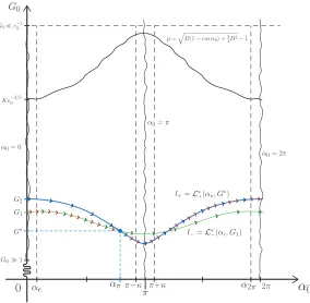
[image:31.595.166.450.189.468.2]

inde-pendent. From part (c) of lemma 1.13 α0 should be different from 0 or π and not in the curve given in (1.89). In figure 1.3 is shown schematically the curves in the plane α0G0 that we will avoid in the following procedure.

Figure 1.2: Zone of diffusion

Take (α0 =αǫ, G0 =G1) and apply successively the scattering mapS− defined in (1.74), its

trajectory will follow the level curvel₋ =_L∗

−(αǫ, G1) up to certain α0=απ close to πwhere G0 takes the valueG∗_{. At this moment, we shift to the scattering map} _S

+ defined as well in (1.74). From applying S+ successively, we will get points along the level curve l+ =L∗+(απ, G∗) up to

α0 =α2π close to 2π= 0(mod2π) where G0 takes the value G2 with G2 > G1, by remark 1.14, we know thatG2−G1 =O(e−G

3

0/3). Continuing in this way, we can travel along all the allowed diffusion zoneG1< G0≪1/e0avoiding always to shift from one scattering map to another, in a point of the curve given in (1.89) wheneverG0=O(e−02/3). Using part (a) and (c) of lemma 1.13 we get figure 1.3. The red arrows represent the trajectory that changes from one scattering map to the other.

Inside the domain 1_≪G0≪1/e0 we can obtain diffusion orbits along arbitrary paths, except those which intersect the small regions described in lemma 1.10 and the curves given in lemma 1.13. This mechanism given by the application of scattering maps produce indeed pseudo-orbits, that is, heteroclinc connections between different periodic orbits ˜Λα0,G0 in ˜Λ∞which are commonly known as transition chains after Arnold’s pioneering work [Arn64]. The existence of true orbits of the system which follow closely these transition chains relies on shadowing methods, which are standard for partially hyperbolic periodic orbits (the so-called whiskered tori in the literature) lying on a normally hyperbolic invariant manifold (NHIM). Such shadowing methods are equally applicable in our case, where we have an invariant manifold ˜Λ∞ which is only topologically equivalent to a

(32)

[image:32.595.168.452.84.362.2]

Figure 1.3: Mechanism for diffusion

With all these elements, we can now state our main results Theorem 1.15. LetG∗

1< G∗2 large enough ande0 small enough. More precisely1≪G∗1< G∗2≪ 1/e0 andµ > 0 small enough. Then, for any G1, G2 ∈(G∗1, G∗2) there exists a trajectory of the

ERTBP such thatG(0)< G1,G(T)> G2 for someT >0.

1.5.3 e0G0

=

λ

,

λ

real positive

To prove diffusion in the casee0G0=λ, forλafixed positive number, we use propositions 1.2 and 1.3 as in section 1.5.1 to compute the scattering map. Nevertheless, we will use the computation of the Melnikov potential given in theorem 1.6, which gives a more involved expression of the scattering map in terms of the Bessel functionsJ0 andJ1. Since the complete computations of the scattering maps are very cumbersome, it will not be possible to provide simple conditions, as in the caseλ≪1, to guarantee the existence of diffusion on the complete zoneA/e0≤G0 ≤B/e0. Thus, in this section, we will see the same mechanism used in section 1.5.1 can be straight forwardly applied, up to some technical conditions that can be checked analytically or numerically.

The Melnikov potential is now given by the same formula (1.48), that is

L(α0, G0, t0;e0) =L0,0(G0) +L0(α0, G0) +L1(α0, G0, t0) +E(α0, G0, t0) (1.97) whereL0,0is the same function as in equation (1.48) and is given by

L0,0(G0) =

π

2G

−3

0 +F1 (1.98)

with

F1=F1(G0) =O(λ2G−05+G− 7

0 ) =O(G− 5

0 ) (1.99)

L0(α0, G0) is also the same function as in equation (1.48) and is given by

L0(α0, G0) =− 15

8 πλG

−6

Global instability in the elliptic restricted three body problem