Evolution in time and scales of the stability of heart interbeat rate
R. Hern´andez-P´erez1, L. Guzm´an-Vargas2, I. Reyes-Ram´ırez2,3and F. Angulo-Brown3 1 SATMEX. Av. de las Telecomunicaciones S/N CONTEL Edif. SGA-II. M´exico, D.F. 09310, M´exico.
2 Unidad Profesional Interdisciplinaria en Ingenier´ıa y Tecnolog´ıas Avanzadas, Instituto Polit´ecnico Nacional, Av.
IPN No. 2580, Col. Ticom´an, M´exico D.F. 07340, M´exico.
3 Departamento de F´ısica, Escuela Superior de F´ısica y Matem´aticas, Instituto Polit´ecnico Nacional, Edif. No. 9
U.P. Zacatenco, M´exico D. F., 07738, M´exico.
PACS 87.19.Hh– Cardiac dynamics
PACS 89.20.-a– Interdisciplinary applications of physics PACS 89.75.Da– Systems obeying scaling laws
Abstract. - We approach heart interbeat rate by observing the evolution of its stability on
scales and time, using tools for the analysis of frequency standards. In particular, we employ the dynamic Allan variance, which is used to characterize the time-varying stability of an atomic clock, to analyze heart interbeat time series for normal subjects and patients with congestive heart failure (CHF). Our stability analysis shows that healthy dynamics is characterized by at least two stability regions along different scales. In contrast, diseased patients exhibit at least three different stability regions; over short scales the fluctuations resembled white noise behavior whereas for large scales a drift is observed. The inflection points delimiting the first two stability regions for both groups are located around the same scales. Moreover, we find that CHF patients show lower variation of the stability in time than healthy subjects.
Introduction. – Analysis of heart rate variability us-ing nonlinear tools have shown that the heart rate is re-lated to different frequency components derived from a large number of control mechanisms from the autonomous nervous system [1]. Recent evidence of studies of heart rate variability indicates that healthy systems even at rest display highly irregular dynamics with multifractal character [2], and subjects with congestive heart failure (CHF) exhibit changes in this multifractality with time [2]. Moreover, different studies conducted on heart inter-beat have revealed quantitative differences in the fractal organization and correlation properties between healthy and diseased subjects, by using different tools from sta-tistical physics and nonlinear dynamics [2, 3]. Among the methods that have been used for the analysis of heartbeat signals are: detrended fluctuations analysis [4, 5], power spectral density [6],fractal dimension [7,8],multifractality [2, 9], Allan and Fano factors [6, 10], wavelets [1, 11]and excursions [12].
In this work, we are interested in studying the stabil-ity of the heartbeat interval rate by using the Allan vari-ance statistics. The Allan varivari-ance was introduced in the field of time and frequency metrology to quantitatively characterize the frequency fluctuations observed in
ap-R. Hern´andez-P´erezet al.
plying the dynamic Allan variance to: (i) identify nonsta-tionarities in the heart interbeat time series; (ii) quantify the evolution of stability with scales and time; and, (iii) as-sess how these properties change for healthy and diseased subjects.
Our stability analysis shows that healthy dynamics is characterized by at least two stability regions along differ-ent scales. In contrast, diseased patidiffer-ents exhibit at least three different stability regions; over short scales the fluc-tuations resembled white noise behavior whereas for large scales a drift is observed. The inflection points delimiting the first two stability regions for both groups are located around the same scales. Interestingly, we find that CHF patients show lower variation in time of the stability than healthy subjects.
Methods. –
Allan Variance. In time and frequency metrology, the normalized frequency deviation y(t) of the oscilla-tors (most commonly atomic clocks) is defined in terms of the nominal oscillator frequency ν0 and the instan-taneous frequency ν(t) as: y(t) = (ν(t)−ν0)/ν0 [13]. The Allan variance (AVAR) is used as a standard to define quantitatively the stability of an oscillator. The definition of AVAR is given by the expression σ2
y(τ) = 1
2⟨(¯yt+τ−y¯t)2⟩ [13], where τ is the observation interval, the operator⟨· ⟩ denotes time averaging and the average frequency deviation ¯yt is defined as ¯yt = 1τ
∫t+τ
t y(t′)dt′. In discrete time, the AVAR is computed from frequency deviation data with the following estimator: σˆ2
y[k] = 1
2(M−2k+1)
∑M−2k+1
j=1 (¯yk[i+k]−y¯k[i]) 2
[13], whereM is the total number of data points, τ0 is the minimum ob-servation time interval, and the integer k = τ /τ0 repre-sents the discrete-time observation interval typically tak-ing values k = 1,2, . . . ,⌊N/3⌋1 (where ⌊·⌋ denotes inte-ger part), and the averaged frequency values are given by ¯
yk[i]≡ k1
∑i+k−1
j=i y[j]. The AVAR at a particular scale is directly related to the variance of wavelet coefficients at that scale when Haar wavelet filters are used [17].
The frequency deviations of frequency standards are ei-ther systematic or stochastic. The latter are often well described by power-law spectral processes: Sy(f) ∼ fβ; for which AVAR has an interesting property: it exhibits a power-law behavior: σ2
y(τ)∼τη, where the exponents are related byη=−β−1 for−2≤β ≤0 [13]. Another way to write the scaling relation is through the Allan deviation:
σy(τ)∼τη/2∼τµ, (1)
with −0.5 ≤ µ ≤ 0.5, where µ = −0.5 corresponds to white noise,µ= 0 to 1/f noise andµ= 0.5 to Brownian
1It is a convention extensively used in the time and frequency
metrology field, and it is related to the uncertainty in the estimation of the Allan variance, which for a given averaging time is propor-tional to the number of differences that contribute to it.
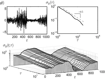
motion2. This scaling property allows the identification of certain stochastic components in a signal (Fig. 1).
200 400 600 800 1000 −5
0 5
t y(t)
100 102 104
10−2 10−1 100
τ σy(τ)
0 200 400 600
800 1000 100
101 100
t τ
σy(t,τ)
−0.5
Fig. 1: (a) Synthetic nonstationary time series representing the frequency deviation of an oscillator(N = 1024); (b) its AVAR,
σy(τ) vs. τ (stability plot); and, (c) its DAVAR (Nw=N/8).
According to AVAR, the signal seems a white noise (µ=−0.5); while, DAVAR captures the nonstationarities and the changes in the variability of the signal.
Dynamic Allan Variance. The dynamic Allan vari-ance (DAVAR) was recently developed for the study of nonstationarities in atomic clocks [15]. It is ob-tained by calculating the estimator ˆσ2
y[k] of AVAR for the data contained in a window of certain length that slides through the data. Thus, DAVAR provides a way to quantify the evolution in time of the stabil-ity. The DAVAR is a deterministic quantity defined as the expected value of the estimator [15]: σˆ2
y[n, k] = 1
2(Nw−2k+1)
∑n+Nw/2−2k
m=n−Nw/2 (¯yk[m+k]−y¯k[m]) 2
, n = t/τ0 is the discrete time,Nw is the length of the analysis win-dow3, the averaged frequency values are computed with ¯
yk[i]≡ 1k
∑i+k−1
j=i y[j], k= 1,2, . . . ,⌊Nw/3⌋ and the sum
runs fromm=n−Nw/2 tom=n+Nw/2−2k−1. The DAVAR isrepresented by a 3-D graph showing the varia-tion of the oscillator’s stability (Fig. 1(c)). Thus, DAVAR at timetcan be interpreted as a representation of the in-stantaneous stability of the oscillator; which is the result of an averaging process on the analysis window of length
Nw[15]. Since noisy signals with power-law spectra follow a scaling law in the AVAR (Eq. 1), understanding whether there are nonstationarities in the clock behavior depends on identifying the changes in the scaling exponentµ.
Heart Rate Dynamics. – There is a debate about
whether it is preferable to analyze heartbeat with refer-ence to real time or to beat number. In Ref. [10], two methods are adapted for analyzing the data from each
2According to the relation between the spectral (β) and Hurst
(H) exponents [6], the following relations hold: µ=H−1 for−1< β≤0 andµ=H, for−2≤β≤ −1
3Selecting the window lengthN
w is a trade-off of two opposite
[image:2.595.350.524.124.255.2]tive “clock” for the timing of the event and that a heart-beat time record can be treated as a point process, i.e., a sequence of events (beats) distributed on the time axis. This approach was followed in Ref. [6], using AVAR to quantify changes in heartbeat time series for heart-failure and normal patients. The second approach emphasizes the interbeat interval and uses the beat number as an index of the biological time.
In the identification of the heartbeat with the frequency deviations of an atomic clock, we use an intermediate ap-proach: what we consider as the input signal is the du-ration of the interbeat interval (time between two con-secutive beats). This signal is indexed with the interval number, on which is based the definition of the “scales”
τ in the AVAR. Thus, the stability is referred to the vari-ation in the durvari-ation of the interbeat interval for differ-ent “scales”. Then, instead of talking about the stability in a certain time scale, we talk about the stability at a certain interbeat scale (certain number of interbeat inter-vals). The advantage of this approach is that it allows studying the evolution of the important quantity: the in-terbeat rate, i.e., the frequency of the oscillator (the heart in this case).
Stability of Heart Oscillations. The concept of home-ostasis, that refers to the tendency of biological systems to maintain a relative constancy of the internal environment (blood sugar, blood pressure and the like) after perturba-tion [18], led to the proposal that physiological variables, such as the cardiac interbeat interval T(n), maintain an approximately constant value in spite of continual pertur-bations. Thus one can write in general T(n) = T0+ξ, where T0 is the preferred level for the interbeat interval and ξ is a white noise with standard deviation σ [18]. Therefore, homeostasis is strongly related to the stability of the heart interbeat intervale rate. Since the heart can be thought of as an oscillator, the applicability of AVAR seems very natural. Therefore, mapping the heart inter-beat to a frequency standard is relevant, and then, apply-ing DAVAR to the heart interbeat time series for healthy and unhealthy subjects would draw some conclusions on the stability of the heart signals; for instance, it allows studying the evolution of the stability of the interbeat rate for both groups.
Evaluating Changes in the Stability of Interbeat Interval Rate. We are interested in quantifying the evolution of stability in scales and time of the heart interbeat rate. For this task we introduce two parameters, namelyµt(τ) and
γτ(t), which are computed from the DAVAR, and repre-sent the change of DAVAR with respect to scale and time, respectively.
The parameterµt(τ) quantifies the local slope, at timet fixed, of DAVAR with respect to the scaleτ, i. e., changes in the slope of DAVAR (in the plane logσy(t, τ) vs logτ)
µt(τ)≡
∂logσy(t, τ)
∂logτ t, (2)
which can be estimated by:
ˆ
µt(τ) =
∆ log ˆσy(t, τ)
∆ logτ . (3)
Notice thatµt(τ) represents the instantaneous exponent of the scaling law in the Allan deviation (Eq. 1). This pa-rameteris similar to the one used in Ref. [10] to estimate the deviation from power-law scaling by applying the Al-lan factor to the counts of the number of beats.
On the other hand, the parameterγτ(t) quantifies the local slope, at scaleτfixed, of DAVAR with respect to time
t, i. e., changes in DAVAR over time (different analysis windows) for a fixed scale. It is defined as:
γτ(t)≡
(
∂σy(t, τ)
∂t
)
τ
, (4)
which is estimated by:
ˆ
γτ(t) =
∆ˆσy(t, τ)
∆t . (5)
Both parameters µt(τ) and γτ(t) will produce a three-dimensional surface, representing the variation of the heart interbeat rate stability in scale and in time, respec-tively.
Results. – We analyze RR interval sequences from
two groups: 16 healthy subjects and 12 CHF patients [19], with 6 hours of diurnal ECG records each with length
N ∼30000 beats (Fig. 2). Notice that the normal sub-ject exhibits a higher variability than the CHF patient, although the latter exhibits more spikes and jumps than for the normal subject. This database is an extended set of records which we have used in previous studies [9, 12]. We compute DAVAR for each time series, considering win-dows withNw=⌊N/30⌋ ∼1000 points, with steps of size
⌊Nw/4⌋ ∼ 250 points and for scales k = 1,2, . . . , kmax, with kmax = ⌊Nw/3⌋ ∼ 333 points. This selection, af-ter computing other options, allows having enough data points to have good confidence in the estimation of AVAR and tracking quick variations in the signals [15].
R. Hern´andez-P´erezet al.
0.5 1 1.5 2 2.5 3
x 104 0.4
0.6 0.8 1 1.2 1.4
RR interval
(a)
0.5 1 1.5 2 2.5 3
x 104 0.4
0.6 0.8 1 1.2 1.4
RR interval
[image:4.595.62.289.87.175.2](b)
Fig. 2: Diurnal records of (a) a normal subject and (b) a CHF patient.
Since both parametersµt(τ) andγτ(t) provide a surface, thus, to summarize the results for each group, we aver-aged them over time, denoted by⟨·⟩t, and over scales, de-noted by⟨·⟩τ; such that averaging over time(scales) gives the mean value of the parameter for a certain scale(time). Figures 5(a) and (b) show the average values forµt(τ) for records of normal and CHF subjects, respectively, with time-averages shown in the main plots, and scale-averages in the insets. The behaviour of the averages for each group of subjects is remarkably different. For normal subjects, two inflection points are observed for the average scal-ing exponentµover the scales (resulting in three regions), while for the CHF patients there are three inflection points (leading to four regions). The first two inflection points for each group occur approximately at the same scales: ∼10 and∼60 interbeat intervals, respectively, while the third inflection point for the CHF group occurs at∼120 inter-beat intervals. Inflection points at∼60 beats is consistent with previous studies [20]. Moreover, scale-averages for normal subjects are negative, while for CHF subjects they fluctuate around zero. The time average values for ¯µt(τ) for the CHF patients have higher dispersion than for nor-mal subjects. Moreover, for both groups the time-average for the shortest scale, i. e., few consecutive interbeat in-tervals, has a significant different value and the largest dispersion than for other scales. On the other hand, Figs. 5(c) and (d) show that both average values of γ¯τ(t) for normal subjects have higher dispersion than for CHF pa-tients, indicating that on average the variation ofσy(t, τ) from one time(scale) to another, for a given scale(time), is more dependent on the value of scale(time). In con-trast,the corresponding average values for CHF patients have lower dispersion. Thus, the local stability for heart interbeat of normal subjects tends to change in timeand scalesdifferently with respect to thetime andscales, than for CHF patients for which a more regular evolution of stability in time and scalesis observed.
Furthermore, for analyzing the scales and time evolu-tion, we compare the value of both µt(τ) and γτ(t) for selected combinations of scales and time. For instance, for the short-term (standing at the first analysis window) and the long-term (last analysis window), we pick values ofµt(τ) for short (µτS) and large (µτL) scales (Figs. 6(a)
[image:4.595.376.491.442.714.2]and (b), respectively). Similarly, for the shortest and the
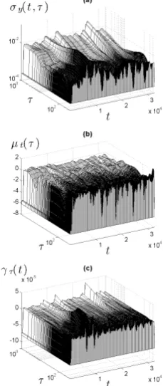
Fig. 3: Stability analysis for a normal subject (Fig. 2(a)): (a) the DAVAR profile; (b)µt(τ), where each line corresponds to
an analysis window (time fixed); and, (c)γτ(t), where each line
corresponds to one scale.
0 50 100 150 200 −0.8
−0.4
τ h¯µit
0 1 2 3
x 104
−0.5 0 0.5
t h¯µiτ
0 50 100 150 200
−0.8 −0.4
τ
h¯µit
0 1 2 3
x 104
−0.5 0 0.5
t
h¯µiτ
0 50 100 150 200
−5 −4 −3 −2 −1 0 1 2x 10
−6
τ
h¯γit
0 1 2 3
x 104
−1 0 1x 10
−4
t
hγ¯iτ
(c)
0 50 100 150 200
−5 −4 −3 −2 −1 0 1 2x 10
−6
τ
h¯γit
0 1 2 3
x 104
−1 0 1x 10
−4
t
h¯γiτ
[image:5.595.48.269.87.255.2](d)
Fig. 5: Average values of parametersµt(τ) andγτ(t) for (a),(c)
normal and (b),(d) CHF subjects. Time-average is show in the main plots, and scale-average in the insets.
largest scales, we pick values for the short (µtS) and the
long (µtL) terms (Fig. 6(c) and (d), respectively). The
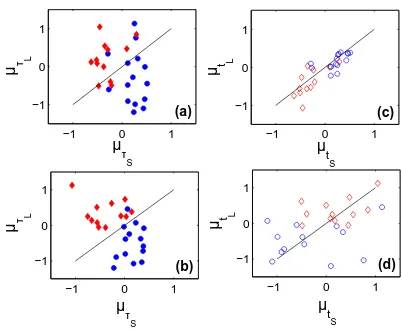
same approach is applied to γτ(t) (Fig. 7). For the scal-ing exponentµt(τ) (Figs. 6(a) and (b)), we observe that for healthy subjects the values for the small scales are slightly larger than for large scales; while for CHF pa-tients the values from small scales are quite larger than for large ones. The values of µt(τ) for healthy subjects are significantly different than for CHF patients (p-value
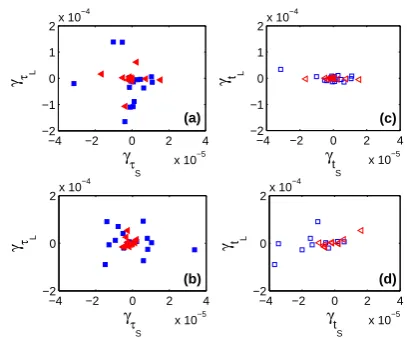
<0.05 by t-Student test). For small-scales (Fig. 6(c)), the scaling exponents are almost over the identity line for both groups indicating low variation with time. Moreover, for the healthy group the scaling exponents are positive, while for the CHF group is the opposite. For large scales (Fig. 6(d)), the scaling exponents are more spread. For the vari-ation in time for DAVAR, expressed byγτ(t), we observe for short- and long-terms (Fig. 7(a) and (b)) a cluster around zero for CHF patients (specially for the short-term), while for normal subjects the values are spread. In this case, we have not found statistical difference be-tween both groups. A similar clustering around zero is observed also for CHF patients for values corresponding to small and large scales (Figs. 7(c) and (d)). For healthy subjects, the values for small scales are also clustered al-though at a less extent, however, at large scales they are spread out at a higher extent than for CHF group.
Discussion. – Some previous studies have
ap-proached heart interbeat by using the so-called Allan fac-tor, based in AVAR, calculated over the number of beats counted in boxes of length T, considering the heart beat dynamics as apoint process[6,10]. However, the approach followed in these studies does not take advantage of the property of the AVAR to quantify the frequency stability of an oscillator. Moreover, the previous studies did not performed adynamicanalysis, i.e., an investigation of the time evolution of stability. The stability of a frequency
−1 0 1
−1 0
µτ S
(a) µ τ L
µ τ L
−1 0 1
−1 0 1
µτ S
(b)
−1 0 1
−1 0
µt S
µ t L
(c)
µ t L
−1 0 1
−1 0 1
µt S
[image:5.595.313.514.88.253.2](d)
Fig. 6: Scatter plots of the DAVAR scaling exponent, repre-sented byµt(τ), for normal (circles) and CHF (diamonds)
sub-jects: (a) short-term, (b) long-term, (c) short-scale, and (d) large-scale.
standard, as quantified by AVAR, tells us the deviation of the oscillator’s frequency from its nominal value, at a certain observation period (scale) τ. Thus, a low value of AVAR indicates a more precise frequency standard (more stable oscillator), and also the variation of AVAR for dif-ferent scalesτ indicates the behavior of the stability.
We found three scaling regions for the DAVAR for the healthy group and four for the CHF group, where the first two regions are delimited by inflection points at around the same scale (number of interbeat intervals). However, the values of the time-averaged scaling exponent ⟨µ⟩t in each of these regions are remarkably different between the groups. The behavior is opposite between the groups in the first two regions, while in the third one, the values of
R. Hern´andez-P´erezet al.
−4 −2 0 2 4
x 10−5 −2
−1 0 1 2x 10
−4
γτ S
γ τ L
(a)
−4 −2 0 2 4
x 10−5 −2
0 2x 10
−4
γτ S
γ τ L
(b)
−4 −2 0 2 4
x 10−5 −2
−1 0 1 2x 10
−4
γt S
γ t L
(c)
−4 −2 0 2 4
x 10−5 −2
0 2x 10
−4
γt S
γ t L
[image:6.595.65.269.82.251.2](d)
Fig. 7: Scatter plots of the time variation of DAVAR, rep-resented by γτ(t), for normal (squares) and CHF (triangles)
subjects: (a) short-term, (b) long-term, (c) short-scale, and (d) large-scale.
Moreover, the evolution of the DAVAR profile for both groups is captured by the scatter plots forµt(τ) andγτ(t). For a stationary signal, we would expect to see a cluster around a certain value ofµt(τ). However, if the signal had different nonstationary features or correlated components, there would be larger dispersions or deviations from the identity line in the scatter plots. However, regarding pa-rameter µt(τ), we observe that for healthy subjects the scaling exponent for the small scales is slightly larger than for large scales; while for CHF patients we identify two regions with opposite behaviors. Thus, CHF signals have stochastic components close to white noise. These compo-nents dominate for small scales for which it corresponds a lower value of the scaling exponent (close to−0.5), which is consistent with other approaches [7]. This is not the case for healthy subjects, for which more long-correlated components are present, whose scaling exponent is larger.
Conclusions. – We map the heart to an oscillator
and then we perform a stability analysis of the heart in-terbeat interval rate, using tools developed for the char-acterization of the frequency stability of frequency stan-dards. In particular, we employ the dynamic Allan vari-ance (DAVAR) to analyze heart interbeat time series for normal subjects and patients with CHF. We find that DAVAR can discriminate the heart interbeat dynamics be-tween both groups. Moreover, the evolution of stability in scales and time is revealed by DAVAR and its numeri-cal partial derivatives. We consider that the DAVAR can contibute to the study of heart interbeat, not only for its computational simplicity but also for its ability to quan-tify the local stability and to reveal the nonstationarities in the signals. For making it useful for clinical usage, fur-ther work has to be performed to characterize the DAVAR profiles for several cardiopathies.
∗ ∗ ∗
We thank L. Galleani for helpul advice and discussion; and the anonymous referees whose suggestions led to im-provement of the manuscript. This work was partially sup-ported by CONACYT (Grant 49128-F-26020), COFAA-IPN, EDI-COFAA-IPN, M´exico.
REFERENCES
[1] Ivanov P. C., Amaral L. A. N., Goldberger A. L.,
Havlin S., Rosenblum M. G., Stanley H. E. and
Struzik Z. R.,Chaos,11(2001) 641.
[2] Ivanov P. C., Amaral L. A. N., Goldberger A. L.,
Havlin S., Rosenblum M. G., Struzik Z. R.and
Stan-ley H. E.,Nature,399(1999) 461.
[3] Goldberger A. L., Amaral L. A. N., Hausdorff
J. M., Ivanov P. C., Peng C. K.andStanley H. E.,
Proc. Natl. Acad. Sci.,99(2002) 2466.
[4] Kantelhardt J. W., Ashkenazy Y., Ivanov P. C.,
Bunde A., Havlin S., Penzel T., Peter J.-H. and
Stanley H. E.,Phys. Rev. E,65(2002) 051908.
[5] Karasik R., Sapir N., Ashkenazy Y., Ivanov P. C.,
Dvir I., Lavie P. and Havlin S., Phys. Rev. E , 66
(2002) 062902.
[6] Turcott R. G.andTeich M. C.,Ann. Biomed. Eng.,
24(1996) 269.
[7] Guzm´an-Vargas L., Calleja-Quevedo E. and
Angulo-Brown F.,Fluct. Noise Lett.,3(2003) 83.
[8] Schmitt D. T.andIvanov P. C.,Am. J. Physiol. Regul.
Integr. Comp. Physiol.,293(2007) 1923.
[9] Guzm´an-Vargas L., Mu˜noz-Diosdado A. and
Angulo-Brown F.,Physica A,348(2005) 304.
[10] Viswanathan G. M., Peng C. K., Stanley H. E.and
Goldberger A. L.,Phys. Rev. E.,55(1997) 845.
[11] Ivanov P. C., Rosenblum M. G., Peng C.-K., Mietus
J., Havlin S., Stanley H. E.andGoldberger A. L.,
Nature,383(1996) 323.
[12] Reyes-Ram´ırez I. and Guzm´an-Vargas L.,Europhys.
Lett.,89(2010) 38008.
[13] Allan D. W.,IEEE Trans. Ultras. Ferr. and Freq.
Con-trol ,34(1987) 647.
[14] Rutman J.,Proc. IEEE,66(1978) 1048.
[15] Galleani L.andTavella P.,IEEE Trans. Ultras. Ferr.
and Freq. Control,56(2009) 450.
[16] Bernaola-Galv´an P., Ivanov P. C., Nunes Amaral
L. A. and Stanley H. E.,Phys. Rev. Lett. ,87(2001)
168105.
[17] Percival D. B. and Walden A. T., Wavelet Methods
for Time Series Analysis (Cambridge University Press,
New York) 2000.
[18] Ivanov P. C., Nunes Amaral L. A., Goldberger
A. L. and Stanley H. E.,Europhys. Lett. , 43(1998)
363.
[19] Goldberger A. L., Amaral L. A. N., Glass L.,
Haus-dorff J. M., Ivanov P. C., Mark R. G., Mietus J. E.,
Moody G. B., Peng C.-K.andStanley H. E.,
Circu-lation ,101(2000) e215.
[20] P.Ch. Ivanov, A. Bunde, L.A.N. Amaral, S. Havlin,
J. Fritsch-Yelle, R.M. Baevsky, H.E. Stanleyand