Kluwer – Handbook of Biomedical Image Analysis Vol.3

(1)

(2)

(3)

Series Editor: Evangelia Micheli-Tzanakou Rutgers University

Piscataway, New Jersey

Signals and Systems in Biomedical Engineering: Signal Processing and Physiological Systems Modeling Suresh R. Devasahayam

Models of the Visual System

Edited by George K. Hung and Kenneth J. Ciuffreda

PDE and Level Sets: Algorithmic Approaches to Static and Motion Imagery Edited by Jasjit S. Suri and Swamy Laxminarayan

Frontiers in Biomedical Engineering:

Proceedings of the World Congress for Chinese Biomedical Engineers Edited by Ned H.C. Hwang and Savio L-Y. Woo

Handbook of Biomedical Image Analysis: Volume I: Segmentation Models Part A

Edited by Jasjit S. Suri, David L. Wilson, and Swamy Laxminarayan Handbook of Biomedical Image Analysis:

Volume II: Segmentation Models Part B

Edited by Jasjit S. Suri, David L. Wilson, and Swamy Laxminarayan Handbook of Biomedical Image Analysis:

Volume III: Registration Models

Edited by Jasjit S. Suri, David L. Wilson, and Swamy Laxminarayan

(4)

Handbook of Biomedical

Image Analysis

Volume III: Registration Models

Edited by

Jasjit S. Suri

Department of Biomedical Engineering Case Western Reserve University Cleveland, Ohio

David L. Wilson

Department of Biomedical Engineering Case Western Reserve University Cleveland, Ohio

and

Swamy Laxminarayan

Institute of Rural Health

Idaho State University Pocatello, Idaho

Kluwer Academic / Plenum Publishers

(5)

䉷2005 Kluwer Academic / Plenum Publishers, New York 233 Spring Street, New York, New York 10013 http://www.wkap.nl/

10 9 8 7 6 5 4 3 2 1

No part of this book may be reproduced, stored in a retrieval system, or transmitted in any form or by any means, electronic, mechanical, photocopying, microﬁlming, recording, or otherwise, without written permission from the Publisher, with the exception of any material supplied speciﬁcally for the purpose of being entered and executed on a computer system, for exclusive use by the purchaser of the work.

Permissions for books published in Europe: [email protected]

(6)

his youngest uncle Paramjeet Chadha and his immediate family: his late sister Sharan, his late brother Amarjeet, and his

late parents Kulwant Kaur and Udam S. Chadha (Fellow of Royal Institute of London).

David Wilson dedicates this handbook to his family and students.

Swamy Laxminarayan dedicates

this book in memory of his beloved parents who were a constant source of inspiration in his life and to his in-laws

(7)

Jasjit S. Suri, Ph.D.

Case Western Reserve University, Cleveland, OH, USA

David L. Wilson, Ph.D.

Baowei Fei, Ph.D

Swamy Laxminarayan, DSc.

State University of Idaho, Pocatello, ID, USA

Andrew Laine, Ph.D.

Columbia University, New York, NY, USA

Elsa Angelini, Ph.D.

Yinpeng Jin, Ph.D.

Aly A. Farag, Ph.D.

University of Louisville, Louisville, KY, USA

Sameh M. Yamany, Ph.D.

Jeremy Nett, M.S.

Thomas Moriarty, M.D., Ph.D.

Stephen Hushek, Ph.D.

Robert Falk, M.D.

A. Ardeshir Goshtasby, Ph.D.

Wright State University, Dayton, OH, USA

Pierre Hellier, Ph.D.

IRISA-INRIA, Cedex, France

Michael Unser, Ph.D.

Swiss Federal Institute of Technology, Lausanne Lausanne, Switzerland

(8)

Jan Kybic, Ph.D.

Czech Technical University, Prague, Czech Republic

Jeff Weiss, Ph.D.

University of Utah, Utah, UT, USA

Nikhil Phatak, Ph.D.

Alex Veress, Ph.D.

Xiao-Hong Zhu, M.S.

University Name, City, State, USA

Yang Ming Zhu, Ph.D.

Philips Medical Systems, Cleveland, OH, USA

Steven M. Cochoff, M.S.

Philips Medical Systems, Cleveland, OH, USA

Torsten Rohlﬁng, Ph.D.

Stanford University, Stanford, CA, USA

Robert Brandt, Ph.D.

Visual Concepts GmbH, Berlin, Germany

Randolf Menzel, Ph.D.

Freie Universit ¨at Berlin, Berlin, Germany

Daniel B. Russakoff, M.Sc.

Calvin R. Maurer, Jr., Ph.D.

Gary E Christensen, DSc.

The University of Iowa, Iowa, USA

Jundong Liu, Ph.D.

Ohio University, Athens, OH

Chi-Hsiang Lo, Ph.D.

National Ilan University, Ilan, Taiwan

Yujun Guo, M.S.

Kent State University, Kent, OH, USA

Cheng-Chang Lu, Ph.D.

Kent State University, Kent, OH, USA

Chi-Hua Tung, Ph.D.

(9)

This book is the result of collective endeavors from several noted engineering and computer scientists, mathematicans, medical doctors, physicists, and radi-ologists. The editors are indebted to all of their efforts and outstanding scientiﬁc contributions. The editors are particularly grateful to Drs. Petia Reveda, Alex Falco, Andrew Laine, David Breen, David Chopp, C. C. Lu, Gary E. Christensen, Dirk Vandermeulen, Aly A Farag, Alejandro Frangi, Gilson Antonio Giraldi, Gabor Szekely, Pierre Hellier, Gabor Herman, Ardeshir Goshtasby, Jan Kybic, Jeff Weiss, Jean-Claude Klein, Majid Mirmehdi, Maria Kallergi, Yang-ming Zhu, Sunanda Mitra, Sameer Singh, Alessandro Sarti, Xioping Shen, Calvin R. Maurer, Jr., Yoshinobu Sato, Koon-Pong Wong, Avdhesh Sharma, Rakesh Sharma, and Chun Yuan and their team members for working with us so closely in meeting all of the deadlines of the book. We would like to express our appreciation to Kluwer Publishers for helping create this invitational handbook. We are particu-larly thankful to Aaron Johnson, the acquisition editor, and Shoshana Sternlicht for their excellent coordination of the book at every stage.

Dr. Suri thanks Philips Medical Systems, Inc., for the MR datasets and en-couragements during his experiments and research. Special thanks are due to Dr. Larry Kasuboski and Dr. Elaine Keeler from Philips Medical Systems, Inc., for their support and motivations. Thanks are also due to my past Ph.D. committee research professors, particularly Professors Linda Shapiro, Robert M. Haralick, Dean Lytle, and Arun Somani, for their encouragements.

We extend our appreciations to Drs. Ajit Singh, Siemens Medical Sys-tems, George Thoma, Chief Imaging Science Division from National Institutes of Health, Dr. Sameer Singh, University of Exeter, UK for his motivations.

(10)

Special thanks go to the Book Series Editor, Professor Evangelia Micheli-Tzanakou, for advising us on all aspects of the book.

We thank the IEEE Press, Academic Press, Springer Verlag Publishers, and several medical and engineering journals for o permitting us to use some of the images previously published in these journals.

Finally, Jasjit Suri thanks his wife Malvika Suri for all the love and support she has showered over the years and to our baby Harman whose presence is always a constant source of pride and joy. I also express my gratitude to my father, a mathematician, who inspired me throughout my life and career, and to my late mother, who most unfortunately passed away a few days before my Ph.D. graduation, and who so much wanted to see me write this book. I love you, Mom. Special thanks to Pom Chadha and his family, who taught me life is not just books. He is my of my best friends. I would like to also thank my in-laws who have a special place for me in their hearts and have shown lots of love and care for me.

David Wilson acknowledges the support of the Department of Biomedical Engineering, Case Western Reserve University, in this endeavor. Special thanks are due to the many colleagues and students who make research in biomedical engineering an exciting, wondrous endeavor.

(11)

Our goal is to develop automated methods for the segmentation of three-dimensional biomedical images. Here, we describe the segmentation of con-focal microscopy images of bee brains (20 individuals) by registration to one or several atlas images. Registration is performed by a highly parallel imple-mentation of an entropy-based nonrigid registration algorithm using B-spline transformations. We present and evaluate different methods to solve the corre-spondence problem in atlas based registration. An image can be segmented by registering it to an individual atlas, an average atlas, or multiple atlases. When registering to multiple atlases, combining the individual segmentations into a ﬁnal segmentation can be achieved by atlas selection, or multiclassiﬁer decision fusion. We describe all these methods and evaluate the segmentation accuracies that they achieve by performing experiments with electronic phantoms as well as by comparing their outputs to a manual gold standard.

The present work is focused on the mathematical and computational the-ory behind a technique for deformable image registration termed Hyperelastic Warping, and demonstration of the technique via applications in image registra-tion and strain measurement. The approach combines well-established princi-ples of nonlinear continuum mechanics with forces derived directly from three-dimensional image data to achieve registration. The general approach does not require the definition of landmarks, fiducials, or surfaces, although it can ac-commodate these if available. Representative problems demonstrate the robust and flexible nature of the approach.

Three-dimensional registration methods are introduced for registering MRI volumes of the pelvis and prostate. The chapter ﬁrst reviews the applications,

(12)

challenges, and previous methods of image registration in the prostate. Then the chapter describes a three-dimensional mutual information rigid body reg-istration algorithm with special features. The chapter also discusses the three-dimensional nonrigid registration algorithm. Many interactively placed control points are independently optimized using mutual information and a thin plate spline transformation is established for the warping of image volumes. Nonrigid method works better than rigid body registration whenever the subject position or condition is greatly changed between acquisitions.

This chapter will cover 1D, 2D, and 3D registration approaches both rigid and elastic. Mathematical foundation for surface and volume registration ap-proaches will be presented. Applications will include plastic surgery, lung can-cer, and multiple sclerosis.

Flow-mediated dilation (FMD) offers a mechanism to characterize endothe-lial function and therefore may play a role in the diagnosis of cardiovascular diseases. Computerized analysis techniques are very desirable to give accuracy and objectivity to the measurements. Virtually all methods proposed up to now to measure FMD rely on accurate edge detection of the arterial wall, and they are not always robust in the presence of poor image quality or image artifacts. A novel method for automatic dilation assessment based on a global image analysis strategy is presented. We model interframe arterial dilation as a super-position of a rigid motion model and a scaling factor perpendicular to the artery. Rigid motion can be interpreted as a global compensation for patient and probe movements, an aspect that has not been sufﬁciently studied before. The scal-ing factor explains arterial dilation. The ultrasound (US) sequence is analyzed in two phases using image registration to recover both transformation models. Temporal continuity in the registration parameters along the sequence is en-forced with a Kalman ﬁlter since the dilation process is known to be a gradual physiological phenomenon. Comparing automated and gold standard measure-ments we found a negligible bias (0.04%) and a small standard deviation of the differences (1.14%). These values are better than those obtained from manual measurements (bias=0.47%, SD=1.28%). The proposed method offers also a better reproducibility (CV =0.46%) than the manual measurements (CV = 1.40%).

(13)

due to surgical procedure, intersubject comparison to build anatomical atlases, etc. Numerous registration techniques have been developed and can be broadly decomposed into intensity-based (photometric) and landmark-based (geomet-rical) techniques. This chapter will present up-to-date methods.

This chapter will then present how segmentation and registration methods can cooperate: accurate and fast segmentation can be obtained using nonrigid registration; nonrigid registration methods can be constrained by segmentation methods. Results of these cooperation schemes will be given.

This chapter will ﬁnally be concerned with validation of nonrigid registration methods. More speciﬁcally, an objective evaluation framework will be presented in the particular context of intersubject registration.

This chapter concerns elastic image registration for biomedical applications. We start with an overview and classiﬁcation of existing registration techniques. We revisit the landmark interpolation and add some generalisations. We develop a general elastic image registration algorithm. It uses a grid of uniform B-splines to describe the deformation. It also uses B-splines for image interpolation. Mul-tiresolution in both image and deformation model spaces yields robustness and speed. We show various applications of the algorithm on MRI, CT, SPECT and ul-trasound data. A semiautomatic version of the registration algorithm is capable of accepting expert hints in the form of soft landmark constraints.

(14)

1. Medical Image Registration: Theory, Algorithm, and Case Studies in

Surgical Simulation, Chest Cancer, and Multiple Sclerosis. . . . 1

Aly A. Farag, Sameh M. Yamany, Jeremy Nett, Thomas Moriarty, Ayman El-Baz, Stephen Hushek, and Robert Falk

2. State of the Art of Level Set Methods in Segmentation and Registration of Medical Imaging Modalities. . . . 47 Elsa Angelini, Yinpeng Jin, and Andrew Laine

3. Three-Dimensional Rigid and Non-Rigid Image Registration for the Pelvis and Prostate. . . . 103 Baowei Fei, Jasjit Suri, and David L. Wilson

4. Stereo and Temporal Retinal Image Registration by Mutual Information Maximization. . . . 151 Xiao-Hong Zhu, Cheng-Chang Lu, and Yang-Ming Zhu

5. Quantiﬁcation of Brain Aneurysm Dimensions from CTA for Surgical Planning of Coiling Interventions. . . . 185

M´onica Hern´andez, Alejandro F. Frangi, and Guillermo Sapiro

6. Inverse Consistent Image Registration. . . . 219 G. E. Christensen

7. A Computer-Aided Design System for Segmentation of Volumetric Images 251 Marcel Jackowski and Ardeshir Goshtasby

8. Inter-subject Non-rigid Registration: An Overview with Classiﬁcation and the Romeo Algorithm. . . . 273 Pierre Hellier

(15)

9. Elastic Registration for Biomedical Applications. . . . 339

Jan Kybic and Michael Unser

10. Cross-Entropy, Reversed Cross-Entropy, and Symmetric Divergence

Similarity Measures for 3D Image Registration: A Comparative Study. . . 393 Yang-Ming Zhu and Steven M. Cochoff

11. Quo Vadis, Atlas-Based Segmentation?. . . . 435 Torsten Rohlﬁng, Robert Brandt, Randolf Menzel, Daniel B. Russakoff,

and Calvin R. Maurer, Jr.

12. Deformable Image Registration with Hyperelastic Warping. . . . 487 Alexander I. Veress, Nikhil Phatak, and Jeffrey A. Weiss

13. Future of Image Registration. . . . 535 Jasjit Suri, Baowei Fei, David Wilson, Swamy Laxminarayan,

Chi-Hsiang Lo, Yujun Guo, Cheng-Chang Lu, and Chi-Hua Tung

The Editors. . . . 555

(16)

Medical Image Registration: Theory,

Algorithm, and Case Studies in Surgical

Simulation, Chest Cancer, and

Multiple Sclerosis

Aly A. Farag,

1

_{Sameh M. Yamany,}

2

_{Jeremy Nett,}

1

_{Thomas Moriarty,}

3

Ayman El-Baz,

1

Stephen Hushek,

4

and Robert Falk

5

1.1 Introduction

Registration found its application in medical imaging due to the fact that physi-cians are frequently confronted with the practical problem of registering medical images. Medical registration techniques have recently been extended to relate multimodal images which makes it possible to superimpose features from differ-ent imaging studies. Registration techniques have been also used in stereotactic surgery and stereotactic radiosurgery that require images to be registered with the physical space occupied by the patient during surgery. New interactive, image-guided surgery techniques use image-to-physical space registration to track the changing surgical position on a display of the preoperative image sets of the patient. In such applications, the speed of convergence of the registration technique is of major importance.

1_{Computer Vision and Image Processing Laboratory, Department of Electrical and}

Com-puter Engineering, University of Louisville, Louisville, KY 40292, USA

2_{System and Biomedical Engineering Department, Cairo University, Giza, Egypt} 3_{Department of Neurological Surgery, University of Louisville, KY 40292, USA} 4_{MRI Department, Norton Hospital, Louisville, KY, USA}

5_{Medical Imaging Division, Jewish Hospital, Louisville, KY, USA}

(17)

Table 1.1: Most important nomenclature used throughout the chapter

x Vector function denoting a point on the model surface y Vector function denoting a point on the experimental surface

S General surface

T Transformation matrix

R Rotation matrix

t Translation vector

d(yi,S) The distance of pointyito shapeS

F() Registration objective function C() The closet point operator GCP() Grid Closest Point transform

G 3D space subset

r Displacement vector in the GCP grid {R,C,H} Coordinates of the GCP grid

δ Grid resolution

Cijk Grid cell

c0ijk Centroid of the cellCijk α,β, andγ 3D-angles of rotations

θ Simplex mesh angle

P 3D point on a free-form surface H Mean curvature of the surface

UP Normal vector at pointP

A Set of landmarks

λ Curvature threshold

E2

n Matching value

O Overlap ratio

s Scale factor

F A medical volume

h() Entropy function

R f A reference medical volume.

(18)

(computed tomography), MRI (magnetic resonance imaging), US (ultrasound), portal images, and (video) sequences obtained by various catheter scopes, e.g., by laparoscopy or laryngoscopy. Other prominent derivative techniques include, MRA (magnetic resonance angiography), DSA (digital subtraction angiography, derived from X-ray), CTA (computed tomography angiography), and Doppler (derived from US, referring to the Doppler effect measured). Functional modal-ities include (planar) scintigraphy, SPECT (single photon emission computed tomography), PET (positron emission tomography), which together make up the nuclear medicine imaging modalities, and fMRI (functional MRI).

An eminent example of the use of registering different modalities can be found in the area of epilepsy surgery [1]. Patients may undergo various MR, CT, and DSA studies for anatomical reference; ictal and interictal SPECT studies; MEG and extra and/or intra-cranial (subdural or depth) EEG, as well as PET studies. Registration of the images from practically any combination will beneﬁt the surgeon. A second example concerns radiotherapy treatment, where both CT and MR can be employed. The former is needed to accurately compute the radiation dose, while the latter is usually better suited for delineation of tumor tissue.

Yet, a more prominent example is the use of medical registration for the same modality, i.e., monomodale registration. For example, in the qualitative evaluation of multiple sclerosis (MS) studies, where multiple MRI scans of the same patient at different times must be compared with one another. Due to the largely arbitrary positioning of the anatomy in the scanner, in a slice-by-slice comparison between studies, quite different anatomy can by chance be located on the same slice numbers in different studies. The goal of registration, therefore, is to align the anatomy from one scan, to the anatomy from another.

Medical registration spans numerous applications and there exists a large score of different techniques reported in the literature. In what follows is an attempt to classify these different techniques and categorize them based on some criteria.

1.2 Medical Registration Classiﬁcations

(19)

[1] provided a good survey on different classiﬁcation criteria. In this section we will summarize seven basic classiﬁcation criteria commonly used (for more details and further reading see the Maintz and Viergever review).

The seven criteria are: 1. Dimensionality

2. Nature of registration basis 3. Nature of transformation 4. Interaction

5. Optimization procedure 6. Modalities involved 7. Subject

1.2.1 Dimensionality

The main division here is either the scope of the registration involvesspatial dimension onlyor istime seriesalso involved. For spacial registration, there are the (i)3D/3Dregistration where two or more volumes of interest are to be aligned together, the (ii)2D/2Dregistration where two medical images are to be aligned together. In general, 2D/2D registration is less complex than the 3D/3D registration. A more complex one is the (iii)2D/3Dregistration which involves the direct alignment of spatial data to projective data (e.g., a preoperative CT image to an intraoperative X-ray image), or the alignment of a single tomographic slice to spatial data. Time can be another dimension involved when the patient’s images and volumes are to be tracked with time for analysis or monitoring.

1.2.2 Nature of Registration Basis

(20)

the registration of the acquired images is comparatively easy, fast, can usually be automated, and, since the registration parameters can often be computed explicitly, has no need for complex optimization algorithms. The main draw-back of extrinsic registration is that, for good accuracy,invasivemaker (e.g., stereotactic frame or screw markers) objects are used.Non-invasivemarkers (e.g., skin markers individualized foam moulds, head holder frames, or dental adapters) can be used, but as a rule are less accurate.

Intrinsic registration can rely onlandmarksin the images or volumes to be aligned. These landmarks can beanatomicalbased on morphological points on some visible anatomical organ(s), or puregeometrical based. Intrinsic registra-tion can also be based on segmentaregistra-tion results. Segmentaregistra-tion in this case can be

rigidwhere anatomically the same structures (mostly surfaces) are extracted from both images to be registered, and used as sole input for the alignment pro-cedure. They can also bedeformable model basedwhere an extracted structure (also mostly surfaces, and curves) from one image is elastically deformed to ﬁt the second image. The rigid model based approaches are probably the most pop-ular methods due to its easy implementation and fast results. A drawback of rigid segmentation based methods is that the registration accuracy is limited to the ac-curacy of the segmentation step. In theory, rigid segmentation based registration is applicable to images of many areas of the body, yet, in practice, the application areas have largely been limited to neuroimaging and orthopedic imaging.

(21)

ﬂexible, yet more complex and the methods range from using cross correlation, variance minimization, histogram clustering and the famous maximization of mutual information (discussed later in details).

1.2.3 Nature of Transformation

Since the registration process tries to recover the optimal transformation be-tween two candidate subjects, the nature of such transformation categorize the registration procedure to be used. The most commonly used is therigid reg-istration where the transformation involves only translations and rotations. If the transformation maps parallel lines onto parallel lines it is calledaffine. If it maps lines onto lines, it is calledprojective. Finally, if it maps lines onto curves, it is calledcurvedorelastic. Each type of transformation contains as special cases the ones described before it, e.g., the rigid transformation is a special kind of affine transformation. A composition of more than one transformation can be categorized as a single transformation of the most complex type in the composition, e.g., a composition of a projective and an affine transformation is a projective transformation, and a composition of rigid transformations is again a rigid transformation. Also a transformation is calledglobalif it applies to the entire image, andlocalif subsections of the image each have their own transformations defined.

Rigid and afﬁne transformations are generally global, and curved transfor-mations are local. This is due to the physical model underlying the curved trans-formation type. Afﬁne transtrans-formations are typically used in instances of rigid body movement where the image scaling factors are unknown or suspected to be incorrect, such as in MRI images due to geometric distortions. The projective transformation type has no real physical basis in image registration except for 2D/3D registration, but is sometimes used as a constrained-elastic transforma-tion when a fully elastic transformatransforma-tion behaves inadequately or has too many parameters to solve.

1.2.4 Interaction

(22)

registration himself, assisted by software supplying a visual or numerical impres-sion of the current transformation, and possibly an initial transformation guess.

Semi-automatic, where the interaction required can be of two different natures: the user needs to initialize the algorithm, e.g., by segmenting the data, or steer the algorithm, e.g., by rejecting or accepting suggested registration hypotheses.

1.2.5 Optimization Procedure

There exists two possible ways of ﬁnding the transformation parameters. Either they are computeddirectly from the available image information, or they are

looked forbased on a certain optimization criterion. Many applications use more than one optimization technique, frequently a fast but coarse technique followed by an accurate yet slow one (as shown later).

1.2.6 Modalities Involved

Four classes of registration tasks can be recognized based on the modalities that are involved. Inmonomodalapplications, the images to be registered be-long to the same modality, as opposed tomultimodalregistration tasks, where the images to be registered stem from two different modalities. The other two aremodality to modelandmodel to modalityregistration where only one image is involved and the other modality is either a model or the patient himself. The model to modality is used frequently in intraoperative registration techniques. Monomodal tasks are well suited for growth monitoring, intervention veriﬁca-tion, rest-stress comparisons, ictal-interictal comparisons, subtraction imaging (also DSA, CTA), and many other applications. The applications of multimodal registration are abundant and diverse, predominantly diagnostic in nature. A coarse division would be into anatomical-anatomical registration, where images showing different aspects of tissue morphology are combined, and functional-anatomical, where tissue metabolism and its spatial location relative to anatom-ical structures are related.

1.2.7 Subject

(23)

registration where one image is acquired from a single patient, and the other image is somehow constructed from an image information database obtained using imaging of many subjects.

1.3 General Registration Theory

In general, registration is the process by which two or more data sets are brought into alignment. Registration can be deﬁned as“the process of ﬁnding a set of transformation operations between two or more data sets such that the overlap between these sets in a certain common space minimizes a certain optimization criterion”.

The registration problem can be mathematically represented as follows: A parametric shapeS, either a curve segment or a surface, is a vector function,

x: [a,b]→ 3 (1.1) for curves whereaandbare scalars and

x:2→ 3 (1.2) for surfaces. Both curve and surface data sets are usually in the form of, or can be easily converted to, a set of 2D or 3D points, which represent the most general form of 2D or 3D curves and surfaces including free-from curves and surfaces. Let the points in the ﬁrst, or model data set,S, be denoted by{xi|i=1, . . . ,m},

and those in the second, or experimental data set,S, be denoted by{yj|j=

1, . . . ,n}. We want to ﬁnd a transformation matrixTsuch that when applied to

S, the distance from each point on the resulting surface and its corresponding point on the model surfaceSis zero in the noise free case.

For the case of rigid registration (without considering the scaling factor), the transformation matrixTconsists of two components: a rotation matrixR, and a translation vectort. The objective of registration is to determineRandt

such that the following criterion is minimized

F(R,t)=

n

i=1

d2(Ryi+t,S). (1.3)

whered(yi,S) denotes the distance of pointyito shapeS.

(24)

new shape will besimilarto the original shape but at a different scale. It should be noticed that we will use the term similarity transformation to represent a rotation, translation and scaling only, no shear or torsion or other deformable transformations are included.

The minimization of Eq. (1.3) is very difﬁcult becaused(Ryi+t,S) is highly

nonlinear since the correspondence betweenyiandSis not known beforehand.

To understand the challenges involved in solving the registration problem one needs to understand the following:

1. For two data sets, if the transformation from one to the other is pre-cisely known, then the registration process would be trivial. But when the transformation is only approximately known, the problem becomes more difﬁcult. It is here that most researchers have addressed this prob-lem. However, few researchers have attempted to solve the problem when the transformation is totally unknown.

2. The search for an unknown, optimal transformation invariably assumes an initial transformation which is iteratively reﬁned through the minimization of some evaluation function. Such search may lead to a local minimum and, unless a global optimizer is used [3], it is difﬁcult to reach a global solution. 3. For many applications (e.g., intraoperative registration), the registration time can be very critical and near real-time registration process is still needed.

The registration process must compensate for three very important problems, which are translational offset, rotational misalignment, and partial data sets. Error due to translational offset occurs when the coordinate origins of the data sets are not the same point inN-dimensional space. This can be demonstrated by calculating the point by point error of two identical surfaces located at different locations in theN-dimensional space. Even though the data sets are identical, the average experimental data error will be equal to the distance of the offset between the two sets.

(25)

The last major problem that the registration process must address is aligning data sets that represents only a portion of the model data. A correspondence between the experimental data set and the corresponding portion of the model data set must be established before correcting for translation and rotation errors. Once this is accomplished, the error measure must be calculated for only the overlapping portions of the two sets. For example, consider scanning a tooth and attempting to calculate the error between the scanned tooth and a model of an entire human jaw. The registration process must be able to determine which region of the jaw coincides with the scanned tooth, assuming the tooth is distinct enough to distinguish between the other teeth, and then calculate the error measure using only the overlapping regions.

In terms of algorithmic implementations, all of the registration techniques fall under two global implementation categories:distance-basedand feature-basedapproaches. In the distance-based approach, the goal is to calculate the transformation by minimizing a criterion relating the distance between the two data sets. In the feature-based approach some differential properties invariant to rigid transformation (such as gray level value, histogram, curvature, mutual information, entropy, etc.) are often used.

In the following sections we will discuss in some details examples of algo-rithms in both the approaches.

1.4 Distance-based Registration Techniques

Among the distance-based techniques, Besl and McKay [4] proposed the Itera-tive Closest Point (ICP)algorithm which establishes correspondences between data sets by matching points in one data set to the closest points in the other data set. ICP is an elegant way to register different data sets because it is intu-itive and simple. Besl and McKay’s algorithm requires an initial transformation that places the two data sets in approximate registration and operates under the condition that one data set be a proper subset of the other. Since their algorithm looks for a corresponding scene point for every model point, incorrect registra-tion can occur when a model point does not have a corresponding scene point due to occlusion in the scene. Attempts at solving these problems have led to several variants of the original algorithm.

(26)

represent-ing the rotation transformation andt is a vector representing the translation transformation, with their closest points in the model data set. A least-squares estimation is then used to reduce the average distance between the matched points in the two data sets. The algorithm is relatively straightforward and can be summarized as follows:

1. Given a motion transformation that initially aligns two data sets to some degree, a set of correspondence is developed between the points in each set. This is done using a simple metric: for each point in the ﬁrst data set, pick the point in the second set which is closest to it under the current transformation.

2. From this set of correspondence an incremental motion can be computed which further aligns these points to one another.

3. Those two steps are iterated until some convergence criterion is satisﬁed. Figure 1.1 illustrates these steps. The ICP algorithm tries to ﬁnd the opti-mal transformation matrix T between two shapes S and S such that Eq. (1.3) is minimized using the closest point operator in distance calculations as follows:

d(yi,S)= ||yi−C(yi,S)|| (1.4)

whereC(·) is deﬁned as the closest point operator, i.e.,C(·) ﬁnds the closest point in shape S to the pointyi. At each step of the minimization process, a

correspondent point on S has to be found for each pointRyi+t onS. This

makes the operation of registration of order O(mn) and as a result ICP has many drawbacks:

1. One of the main disadvantages of the ICP algorithm is its computation complexity. This makes the algorithm not suitable for applications where near real-time performance is required.

2. The algorithm converges successfully to a local solution but there is no guarantee that it will reach a global solution.

(27)

The initial two surfaces

1– Initial alignment

2– Find correspondence between closest points

3– Calculate an incremental motion

4– Iterate until some convergence criterion is satisfied

Figure 1.1: A diagram illustrating the distance-based registration algorithm steps which start by an initial alignment and then ﬁnding correspondence from which incremental motion is calculated and this process iterates until conver-gence.

Attempts at solving these problems have led to several variants of the original algorithm. In what follows, we provide a review of these improvements. Another good review can be found in [5].

1.4.1 Improving Correspondence

(28)

The first such effort was by Chen and Medioni [7]. They have improved the ICP algorithm by minimizing the distance from the sensed point to the nearest estimated plane approximating the model surface. They begin by finding the data point in the second set that is closest to a line through the point in the first set in the direction of its estimated surface normal. Then the tangent plane at this intersection point is used as the surface approximation. Yet finding the estimated plane involves another iterative procedure which further adds to the computation complexity. They reduced the complexity by selecting some impor-tant points on the smooth surfaces of the object and used these points for the registration. This works well if the smooth surfaces are uniformly distributed over the object, which is not the case for many free-form objects. More accu-rate but time-consuming estimates of the surface have also been used, such as octrees [10], triangular meshes [11], and parametric surfaces [12].

Most researchers have used, the simple Euclidean distance in determining the closest point [3, 4, 6, 7, 8, 9, 11, 12, 13, 14]. Fewer have used higher dimensional feature vectors, such as including the estimated surface normal [15].

1.4.2 Thresholding Outliers

Most of the early algorithms were limited by the original assumption that one data set was a subset of the other [4, 7, 8, 11, 12, 14]. Proposals to bypass this limitation have involved imposing a heuristic threshold on either the distance allowed between points in a valid pairing [6, 9, 10, 13, 15] and the deviation of the surface normals of corresponding points [15]. Any point pairs which exceed these thresholds or constrains are assumed to be incorrect. These thresholds are usually predefined constants related to the estimated accuracy of the initial transformations and can be difficult to choose robustly. Dynamically adjustable thresholds have been based on both the distribution of the distance errors at each iteration [6] and a fuzzy set classification of inlier and outliers correspon-dences [16].

1.4.3 Computational Requirements

In all of the techniques, computing potential correspondences is generally the most time-consuming step. In a brute-force approach [4, 15, 12], an O(N2₎

(29)

the actual time, with a potential loss of accuracy [11], is to subsample the original data sets. Criteria for sub-sampling include taking a simple fraction of the original number [13], using multiple scales of increasing resolution [3], or taking points in areas away from surface discontinuities [7], in areas of fine detail [8], and in small random sets for robust transform estimation [14]. A more accurate and slower alternative is to use the full original data sets, but organize the closest point search using efficient data structures such as the octree [10] and k-d tree [6]. The k-d tree is even more efficient, O(NlogN), when higher order features of the points are incorporated in the distance metric.

1.4.4 Computing Intermediate Motions

Once a set of correspondences has been determined, a motion transform must be computed that best aligns the points. The most common approach is to use one of several least squares techniques to minimize the distances between corre-sponding points [4, 6, 8, 11, 14, 7]. In certain cases [6], individual point contribu-tions are weighted based on the suspected noise of different porcontribu-tions of the data sets. More robust estimation using the least median squares technique (cluster-ing many transforms computed from smaller sets of points) has been tried by Masudaet al.[14]. Alternatively, a Kalman ﬁlter has been used to track the inter-mediate motion at each iteration as new correspondences are computed [6]. More involved techniques compute the motion transform via some form of search in the space of possible transforms, trying to minimize a cost function such as the sum of distance errors across all corresponding points. Movements in transform parameter space are computed based on the changing nature of the function. Such standard search strategies as Levenberg-Marquardt [10, 12], simulated annealing [13] and genetic algorithms [9] have been used. Correspon-dences must be periodically updated during the search to keep the error function current. Updating too frequently can drastically increase the amount of compu-tation, while too few updates can lead to an incorrect minimization.

1.4.5 Initialization and Convergence of Searches

(30)

estimate is determined by a previous process [6, 7, 11, 12, 14], possibly cal-culated using feature sets. Other prior estimates can be given by a rotary ta-ble [10], a robot arm [13], or even the user. Most such estimates are assumed to be quite accurate so that using one of the various distance thresholds during matching will prune outliers correctly. Other researchers do their own feature-based alignment prior to refinement using such characteristics as principal mo-ments [4] or similar triangles on a mesh representation of the data [8]. If these distinguishing features are absent, a uniform distribution of starting points can always be processed [4]. All of the ICP algorithms must use some set of cri-teria to detect convergence of the final transformation. For those techniques that compute intermediate motions using least squares methods, convergence is achieved when the transform implies a sufficiently small amount of mo-tion [6, 8, 14] or the distance between corresponding points becomes suitably close [4, 7, 11, 14]. The iterative searches of parameter space typically converge based on small changes in the parameters or error value, or if the shape of the cost function at the current value indicates a function minimum. Any method can be terminated if convergence is not detected after some maximal number of iterations [3].

1.4.6 A Genetic Distance-based Technique

Another enhancements on the ICP algorithm for fast registration of two sets of 3D curves or surfaces was done by applying a distance transform to the model surface [3, 9]. The distance transform essentially converts the 3D space sur-rounding the two data sets into a ﬁeld in which every point stores the magnitude and direction of a displacement vector from this point to the nearest surface element. Thus the cost function is largely precomputed. Such a transform is called thegrid closest point(GCP) [9]. A genetic algorithm (GA) is then used to minimize the cost function.

Genetic algorithms (GAs) [17] provide a powerful and domain-independent search method for complex, poorly understood search spaces. Genetic algo-rithms have been applied to a wide diversity of problems such as combinatorial optimization [18], VLSI layout [19], machine learning [20], scene recognition [21], and adaptive image segmentation [22].

(31)

point in the experimental data set. This time can be signiﬁcantly reduced by applying the following grid closest point (GCP) transform.

The GCP transformGCP:3→ 3maps each point in the 3D spaceG⊂ 3that encloses the two surfacesSandSto a displacement vector,r, which represents the displacement from the closest point in the model setS. Thus for allz∈G

GCP(z)= r=xm−z (1.5)

such that

d(z,xm)=min

xi∈S

{d(z,xi) (1.6)

whered(·) is the Euclidean distance. For each point inG, the transform calculates a displacement vector to the closest point in the model data set which can be used subsequently to ﬁnd matching points betweenSandSduring the minimization process.

In the discrete case, assume thatGconsists of a rectangular box that encloses the two surfaces. Furthermore, assume thatGis quantized into a set ofL×W × Hcells of sizeδ3

{Cijk|0≤i≤L, 0≤ j≤W, 0≤k≤ H} (1.7)

such that

W =(Wmax−Wmin)/δ (1.8)

L=(Lmax−Lmin)/δ (1.9)

and

H=(Hmax−Hmin)/δ (1.10)

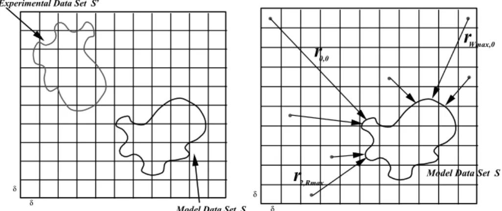
Figure 1.2 shows a 2D illustration of such a grid.

Each cellCijkwill hold a displacement vectorrijkwhich is a vector from its

centroid, denoted byc0ijk, to its closest point in the model set.

The GCP transform is applied only once at the beginning of the registration process. After its application, each cell inG has a displacement vector to its closet point in the model set. During the minimization, to calculate the closest pointx˜ =C(y_v,S) to a pointy_v∈S, you ﬁrst have to ﬁnd the intersection ofy_v

(32)

Model Data Set S δ

δ

Model Data Set S

δ δ

r

0,0

r

Wmax,0

r

2,Rmax Experimental Data Set S,

Figure 1.2: (Left) superimposing a uniform gridGof sizeδonto the space that encloses the model and experimental data sets. (Right) for each cellCijk∈G,

calculate a displacement rijk, from the cell centroid, c0ijk, to its closet point

onS.

pointy_v = {u, v, w}lies can be found by

i= u−Lmin

δ , j=

v−Wmin

δ , k=

w−Hmin

δ (1.11)

If the content of the cellCijkisrijkthen

˜

x=C(y_v,S)= rijk+c0ijk (1.12)

An approximation of the closest point can be obtained by using the point itself instead of the centroid of the cell in which it lies

˜

x=C(y_v,S)≈ rijk+yv (1.13)

Equation (1.13) introduces an error which is a function ofδ, the quantization step. This error can be reduced to some extent by using a non-uniform quantization. It should be noted that the GCP transform is spatially quantized and its accuracy depends largely on the selection ofδ. The error in the displacement vector is

≤ 3 4δ

2_{. Therefore, smaller values for}_δ_{will give higher accuracy but on the extent}

(33)

at the beginning of the registration and ﬁne matching toward the end of the minimization.

The next step is to search for the transformation parameters using genetic algorithms (GAs). GAs, pioneered by Holland [23], are adaptive, domain inde-pendent search procedures derived from the principles of natural population genetics. GAs borrow its name from the natural genetic system. In natural ge-netic system whether a living cell will perform a specific and useful task in a predictable and controlled way is determined by its genetic makeup, i.e., by the instructions contained in a collection of chemical messages called genes [24]. Genetic algorithms are briefly characterized by three main concepts: a Dar-winian notion of fitness or strength which determines an individual’s likelihood of affecting future generations through reproduction; a reproduction operation which selects individuals for recombination to their fitness or strength; and a recombination operation which creates new offspring based on the genetic structure of their parents.

Genetic algorithms work with a coding of a parameter set, not the parameters themselves and search from a population of points, not a single point. Also ge-netic algorithms use payoff (objective function) information, not derivatives or other auxiliary knowledge and use probabilistic transition rules, not determinis-tic ones. These four differences contribute to genedeterminis-tic algorithms’ robustness and resulting advantage over other more commonly used search and optimization techniques (see Fig. 1.3).

Since the genetic algorithm works by maximizing an objective function, the ﬁtness function,Fr(R,t), can be deﬁned as in Eq. (1.3).

Combining (1.3) with the GCP transform to ﬁnd matching points between the two data sets, Eq. (1.3) can be rewritten as

Fr(R,t)= −

n

i=1

d2(y,GCP(y_i)+y_i) (1.14)

wherey_i=Ryi+t. By maximizing (1.14) we effectively minimize (1.3).

The objective of the registration process is to obtain the rotation matrixR

(34)

δ

δ δ/2

δ/2

r

Wmax,0

r

2,Rmax

Figure 1.3: An example of a non-uniform gridG.

In the 2D space, the parameter set is reduced tox,y, and the angle of rotationθ. These parameters are represented by binary notation to minimize as much as possible the length of the schematad(H) and the order of the schemata

O(H). The number of bitsnp, assigned to each parameter, p, depends on the

type of application and the required degree of accuracy. The number of bits should be chosen as small as possible to minimize the time of convergence of the genetic algorithm. For example, you can assign 8 bits each, thus allowing a displacement of±127 units. A range of±31 can also enforced over the angles of rotation. Therefore 6 bits are assigned for each angle of rotation. As shown in Fig. 1.4, the genes are formed from the concatenation of the binary coded parameters.

The selection operator chooses the highest ﬁtted genes for mating using a Roulette wheel selection [24]. The crossover and mutation operators are imple-mented by choosing a random crossover and mutation point with probabilities

Pcp and P p

m, respectively, for each coded parameter p. The generated strings

are concatenated together to form one string from which the populations are formed (see Fig. 1.5).

(35)

∆

x

∆

y

∆

z

α

β

γ

8b 8b 8b 6b 6b 6b

Displacements Rotations

∆

x

∆

y

θ

8b

6b

Displacements Rotation Population

(a)

(b)

Figure 1.4: Different gene structures.

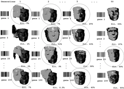
Generations

gene 1

gene 2

gene 25

gene 100 gene 100 gene 100 gene 100

gene 25 gene 25 _{gene 25}

gene 2 gene 2 _{gene 2}

gene 1 gene 1 _{gene 1}

fit. 5%

fit. 1%

fit. 2%

fit. 7% fit. 0.5% fit. 40% fit. 95%

fit. 9% fit. 98% fit. 99%

fit. 10% fit. 60% fit. 97%

fit. 7% fit. 25% fit. 95%

1 2 5 50

. . . . . . . . . . . . . . . . . . . . . . . . . . .

(36)

parameters needed to be known beforehand to efﬁciently code them into a string. Also if the range is large, the GA convergence can be slow.

1.5 Feature-Based Registration Techniques

Feature-based registration techniques rely on extracting and matching similar features vector between two or more data sets in order to ﬁnd corresponding data points. So the two critical procedures involved in feature-based registra-tion is feature extractionand feature correspondence. Feature representations, which are invariant to scaling, rotation, and translation, are more desirable in the matching process.

One of the most successful feature-based registration techniques, espe-cially for multimodal registration, is bymaximization of mutual information

(MI) [25]. This technique works well for both MR and CT since they are infor-mative of the same underlying anatomy and there will be mutual information between the MR image and the CT image. Such a technique would attempt to ﬁnd the registration by maximizing the information that one volumetric image pro-vides about the other. It requires no a priori model of the relationship between the modalities, it only assumes that one volume provides the most information about the other one when they are correctly registered.

Unfortunately, if initial transformation between the two modalities is un-known, the MI will converge slowly. So, we will demonstrate how to use a com-posite registration procedure that integrates another feature-based registration technique, mainly a surface-based[26] registration technique, to estimate the initial transformation. Surface-based registration techniques use features avail-able on the data set surface mesh such as density or curvature. The surface-based registration techniques work better for free-form surfaces, such as the skin contours, while MI works better for voxel-based volumes. Such compos-ite registration procedures have become recently the state-of-the-art in most registration applications due to the fact that most feature-based techniques are complementary in nature.

1.5.1 Surface-Based Registration Algorithm

(37)

Most of the surface representation schemes found in literature have adopted some form of shape parameterization especially for the purpose of object recognition. However, free-form surfaces, in general (e.g., CT/MRI skin con-tours), may not have simple volumetric shapes that can be expressed in terms of parametric primitives. Some representation schemes for free-form surfaces found in literature include the“splash” representation proposed by Stein and Medioni [27] in which the surface curvature along the intersection of the sur-face and a sphere centered at the point of interest is calculated for different sphere diameters and a signature curve is obtained for this point. Also the work of Chua and Jarvis [28], who proposed the“point signature” representation which describes the local underlying surface structure in the neighborhood of a point. This is obtained by plotting the distance proﬁle of a circle of points to a plane deﬁned by that circle of points. Dorai and Jain [29] proposed an-other representation called “COSMOS” for free-form objects in which an ob-ject is described in terms of maximal surface patches of constant shape index from which properties such as surface area, curvedness and connectivity are built into the representation. Johnson and Hebert [30] recently introduced a new representation scheme called the “spin image”. This image represents the histogram of the surface points relative to a certain oriented point. This image is generated for each oriented point on the surface and matching be-tween two surfaces is done by matching the spin images of the points in the two surfaces. Yamany and Farag [26] introduced another technique based on

surface signatures. Surface signatures are 2D images formed by coding the 3D curvature information seen from a local point. These images are invariant to most transformation. In what follows are some details for some of these algorithms.

1.5.1.1 The “Splash” Surface Registration

Geometric indexing have been one of the most used surface indexing techniques because it used the geometrical relationships between invariant features. How-ever, another form of indexing that uses local shape information has become more popular. As it is based on structural information local to the neighborhood of a point, this indexing method is called “Structural indexing”.

(38)

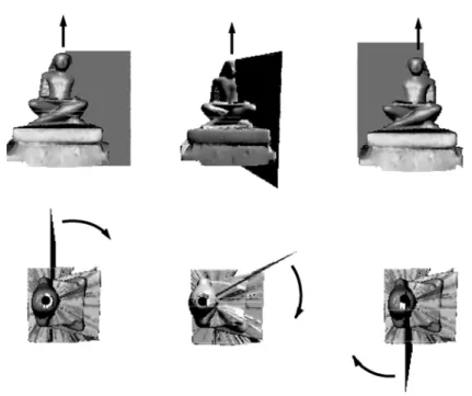
AVERAGE NORMALS

R R

Figure 1.6: An illustration of the “splash” representation scheme. At speciﬁc points on the surface, the intersections of the surface patches and the spheres of preﬁxed radii are obtained. For each intersection a curve representing the average normal of the points in the intersection and the point in study is obtained. These curves are further used for matching.

around a speciﬁc point into a series of contours, each of which is the locus of all points at a certain distance from the speciﬁc point.

(39)

Matching is performed using the contour codes of points on the two surfaces. Fast indexing was achieved by hashing the codes for all models in the library into an index table.

At runtime recognition, the splashes of highly structured regions are com-puted and encoded using the same encoding scheme. Models which contain similar codes as the splashes appearing in the scene are extracted. Veriﬁcation is then performed for each combination of three correspondences.

1.5.1.2 The “Point Signature” Surface Registration

This approach was introduced by Chua and Jarvis [28] for fast recognition. They establish a “signature” for each of the given 3D data points rather than just depending on the 3D coordinates of the point. This is similar to the “splash” representation but instead of using the relationship between the surface normals of the center points and its surrounding neighbors, they used the point set itself. For a given point p, they place a sphere of radius r, centered at p (simi-lar to the method used in splash as depicted in Fig. 1.6). The intersection of the sphere with the object surface is a 3D space curve whose orientation can be defined by a directional frame formed of the normal to the plane fitted to the curve, a reference direction and their cross product. The next step is to sample the points on this curve starting from the reference direction. For each sampled point there exist two information, the distance from itself to the fitted plane and the clockwise angle about the normal from the reference direction. Figure 1.7 shows some typical examples of point signatures for different surface types.

Due to this simple representation, the 3D surface matching is transformed into 1D signature matching. In their paper they analyze this signature matching and estimate the accepted error tolerance in the matched signature. Prior to recognition, the model library is built by computing the point signatures for each point in the model and for every model. They also used hashing to index the signatures in a table. At runtime, the surface under study is sampled at a ﬁxed interval and the sampled points are used in the matching process.

1.5.1.3 The “COSMOS” Surface Registration

(40)

N N

N

N N

N

Ref Ref

Ref

Ref d

θ

d

θ

d

θ

d

θ

d

θ

d

θ

(a) (b) (c)

(d) (e) (f )

Figure 1.7: Examples of point signatures: (a) peak, (b) ridge, (c) saddle, (d) pit, (e) valley, (f) roof edge.

be used to describe sculpted objects, as well as objects composed of simple analytical surface primitives. Second, to be as compact and as expressive as possible for accurate recognition of objects from single range image.

(41)

The patches that get assigned to the same point on the sphere are aggregated according to the shape categories of the surface components.

The concept of “shape spectrum” features is also included in the COSMOS framework. This allows free-form object views to be grouped in terms of the shape categories of the visible surfaces and their surface areas.

For the recognition purpose, COSMOS adapted a feature representation con-sisting of the moments computed from the shape spectrum of an object view. This eliminated unlikely object view matches from a model database of views. Once a small subset of likely candidate views has been isolated from the database, a detailed matching scheme that exploits the various components of the COSMOS representation is performed to derive a matching score and to establish view surface patch correspondence.

1.5.1.4 The “Spin Image” Surface Registration

Johnson and Hebert [30] presented an approach for recognition of complex objects in cluttered 3D scenes. Their surface representation, the “spin” image, comprises descriptive images associated with oriented points on the surface. Using a single point basis, the positions of the other points on the surface are de-scribed by two parameters. These parameters are accumulated for many points on the surface and result in an image at each oriented point which is invariant to rigid transformation.

Through correlation of images, point correspondences between a model and scene data are established. Geometric consistency is used to group the corre-spondences from which plausible rigid transformations that align the model with the scene are calculated. The transformations are then refined and verified using a modified ICP algorithm.

(42)

Figure 1.8: The spin image generation process can be visualized as a sheet spinning around the oriented point basis, accumulating points as it sweeps space.

The term “spin-map” comes from the cylindrical symmetry of the oriented point basis; the basis can spin about its axis with no effect on the coordinates with respect to the basis. To create a spin image, ﬁrst an oriented point on the surface is selected. Then for each other point on the surface, the spin-map pa-rameters are computed. These papa-rameters are then accumulated in a 2D array. Once all the points on the surface have been processed, the 2D array is converted into a gray image. Figure 1.8 shows the spin-image generation process and vi-sualizes it as a sheet spinning around the oriented point basis, accumulating points as it sweeps space. Figure 1.9 shows examples of spin images generated for the surface of a statue. The darker the pixel, the higher the number of points projected into this location.

(43)

Figure 1.9: Examples of spin images generated for the surface of a statue. The darker the pixel, the higher the number of points projected into this location.

1.5.1.5 The “Surface Signature” Surface Registration

The surface signature algorithm captures the 3D curvature information of any free-form surface and encodes it into a 2D image corresponding to a certain point on the surface. This image is unique for this point and is independent from the object translation or orientation in space.

(44)

corresponding points in each surface. A pointP on a surface/curveS, is called

importantpoint, PI, if and only if the absolute value of the curvature at this

point is larger than a certain positive value (a threshold).

A= {PI} = {P ∈S| |Curv(P)|> , >0} (1.15)

As theimportantpoints are landmarks, one may expect that they are stable for the same object. However, due to scanning artifacts, their number and loca-tions may vary. By adjusting the curvature threshold, a common subset can be found. Otherwise, the object has either suffered from non-rigid transformations or its visible surface has no landmarks.

The signature, computed at each important point, encodes the surface cur-vature seen from this point, thus giving it discriminating power. As shown in Fig. 1.10 (a), for each important point P∈ Adeﬁned by its 3D coordinates and the normalUP at the patch wherePis the center of gravity, each other pointPi

on the surface can be related to Pby two parameters: The distance

di= ||P−Pi|| (1.16)

and the angle

αi=cos−1

UP·(P−Pi)

||P−Pi||

(1.17)

Also you can notice that there is a missing degree of freedom in this represen-tation which is the cylindrical angular parameter. At each location in the image, the gray value encodes the angle

βi=cos−1(UP·UPi) (1.18)

This represents the change in the normal at the surface point Pirelative to

the normal atP. Figure 1.10 (b) shows some signature images taken at different important points on the skin model of a patient’s head.

The next step in the registration process is to match corresponding signature images of two surfaces. The ultimate goal of the matching process is to find at least a three-points correspondence in order to calculate the transformation pa-rameters. The benefit of using the signature images to find the correspondence is that we can now use image processing tools in the matching, hence reducing the time taken to find accurate transformation. One such tool isTemplate Matching

(45)

UP

UPi

P

Pi

UP

UPi

di αi βi

SPS image at P

d

α

di

αi

βi

(46)

The end result of the matching process is a list of groups of likely three-points correspondences that satisﬁes the geometric consistency constraint. The list is sorted such that correspondences that are far apart are at the top of the list. A rigid transformation is calculated for each group of correspondences and a veriﬁcation stage [9] is performed to obtain the best group. Detailed discus-sion concerning the surface signature sensitivity and robustness can be found in [26].

1.5.2 Maximization of Mutual Information

(MI) Algorithm

MI is a basic concept from information theory, measuring the statistical depen-dence between two random variables or the amount of information that one variable contains about the other. The MI registration criterion used states that the MI of corresponding voxel pairs is maximal if the two volumes are geometri-cally aligned [31]. No assumptions are made regarding the nature of the relation between the image intensities in either modality.

Consider the two medical volumes to be registered as the reference volume

Rand the floating volume F. A voxel of the reference volume is denotedR(x), wherexis the coordinates vector of the voxel. A voxel of the floating volume is denoted similarly as F(x). Given thatT is a transformation matrix from the coordinate space of the reference volume to the floating volume, F(T(x)) is the floating volume voxel associated with the reference volume voxelR(x).

MI seeks an estimate of the transformation matrix that registers the reference volume Rand ﬂoating volume Fby maximizing their mutual information. The vectorxis treated as a random variable over coordinate locations in the refer-ence volume. Mutual information is deﬁned in terms of entropy in the following way [25]:

I(R(x),F(T(x)))≡h(R(x))+h(F(T(x)))−h(R(x),F(T(x))). (1.19)

where h(R(x)) and h(F(T(x))) are the entropy of R and F, respectively.