The Theory and Practice of Spatial Econometrics

(1)

James P. LeSage

Department of Economics

University of Toledo

(2)

Preface

This text provides an introduction to spatial econometric theory along with numerous applied illustrations of the models and methods described. The ap-plications utilize a set of MATLAB functions that implement a host of spatial econometric estimation methods. The intended audience is faculty,students and practitioners involved in modeling spatial data sets. The MATLAB functions described in this book have been used in my own research as well as teach-ing both undergraduate and graduate econometrics courses. They are available on the Internet at http://www.econ.utoledo.edu along with the data sets and examples from the text.

The theory and applied illustrations of conventional spatial econometric models represent about half of the content in this text,with the other half devoted to Bayesian alternatives. Conventional maximum likelihood estimation for a class of spatial econometric models is discussed in one chapter,followed by a chapter that introduces a Bayesian approach for this same set of models. It is well-known that Bayesian methods implemented with a diﬀuse prior simply reproduce maximum likelihood results,and we illustrate this point. However, the main motivation for introducing Bayesian methods is to extend the conven-tional models. Comparative illustrations demonstrate how Bayesian methods can solve problems that confront the conventional models. Recent advances in Bayesian estimation that rely on Markov Chain Monte Carlo (MCMC) methods make it easy to estimate these models. This approach to estimation has been implemented in the spatial econometric function library described in the text, so estimation using the Bayesian models require a single additional line in your computer program.

Some of the Bayesian methods have been introduced in the regional science literature,or presented at conferences. Space and time constraints prohibit any discussion of implementation details in these forums. This text describes the im-plementation details,which I believe greatly enhance understanding and allow users to make intelligent use of these methods in applied settings. Audiences have been amazed (and perhaps skeptical) when I tell them it takes only 10 seconds to generate a sample of 1,000 MCMC draws from a sequence of condi-tional distributions needed to estimate the Bayesian models. Implementation approaches that achieve this type of speed are described here in the hope that other researchers can apply these ideas in their own work.

I have often been asked about Monte Carlo evidence for Bayesian spatial

(3)

econometric methods. Large and small sample properties of estimation proce-dures are frequentist notions that make no sense in a Bayesian setting. The best support for the eﬃcacy of Bayesian methods is their ability to provide solutions to applied problems. Hopefully,the ease of using these methods will encourage readers to experiment with these methods and compare the Bayesian results to those from more conventional estimation methods.

Implementation details are also provided for maximum likelihood methods that draw on the sparse matrix functionality of MATLAB and produce rapid solutions to large applied problems with a minimum of computer memory. I believe the MATLAB functions for maximum likelihood estimation of conven-tional models presented here represent fast and eﬃcient routines that are easier to use than any available alternatives.

Talking to colleagues at conferences has convinced me that a simple soft-ware interface is needed so practitioners can estimate and compare a host of alternative spatial econometric model speciﬁcations. An example in Chapter 5 produces estimates for ten diﬀerent spatial autoregressive models,including maximum likelihood,robust Bayesian,and a robust Bayesian tobit model. Es-timation,printing and plotting of results for all these models is accomplished with a 39 line program.

Many researchers ignore sample truncation or limited dependent variables because they face problems adapting existing spatial econometric software to these types of sample data. This text describes the theory behind robust Bayesian logit/probit and tobit versions of spatial autoregressive models and geographically weighted regression models. It also provides implementation de-tails and software functions to estimate these models.

Toolboxes are the name given by the MathWorks to related sets of MAT-LAB functions aimed at solving a particular class of problems. Toolboxes of functions useful in signal processing,optimization,statistics,ﬁnance and a host of other areas are available from the MathWorks as add-ons to the standard MATLAB software distribution. I use the termEconometrics Toolbox to refer to my public domain collection of function libraries available at the internet address given above. The MATLAB spatial econometrics functions used to im-plement the spatial econometric models discussed in this text rely on many of the functions in theEconometrics Toolbox. The spatial econometric functions constitute a “library” within the broader set of econometric functions. To use the spatial econometrics function library you need to download and install the entire set ofEconometrics Toolbox functions. The spatial econometrics func-tion library is part of theEconometrics Toolbox and will be available for use along with more traditional econometrics functions. The collection of around 500 econometrics functions and demonstration programs are organized into li-braries,with approximately 40 spatial econometrics library functions described in this text. A manual is available for the Econometrics Toolbox in Acrobat PDF and postscript on the internet site,but this text should provide all the information needed to use the spatial econometrics library.

(4)

estimation results for all of the econometric and spatial econometric functions. This was accomplished using the “structure variables” introduced in MATLAB Version 5. Information from estimation procedures is encapsulated into a single variable that contains “ﬁelds” for individual parameters and statistics related to the econometric results. A thoughtful design by the MathWorks allows these structure variables to contain scalar,vector,matrix,string,and even multi-dimensional matrices as ﬁelds. This allows the econometric functions to return a single structure that contains all estimation results. These structures can be passed to other functions that intelligently decipher the information and provide a printed or graphical presentation of the results.

TheEconometrics Toolboxalong with the spatial econometrics library func-tions should allow faculty to use MATLAB in undergraduate and graduate level courses with absolutely no programming on the part of students or faculty. Prac-titioners should be able to apply the methods described in this text to problems involving large spatial data samples using an input program with less than 50 lines.

Researchers should be able to modify or extend the existing functions in the spatial econometrics library. They can also draw on the utility routines and other econometric functions in the Econometrics Toolbox to implement and test new spatial econometric approaches. I have returned from conferences and implemented methods from papers that were presented in an hour or two by drawing on the resources of theEconometrics Toolbox.

This text has another goal,applied modeling strategies and data analysis. Given the ability to easily implement a host of alternative models and produce estimates rapidly,attention naturally turns to which models best summarize a particular spatial data sample. Much of the discussion in this text involves these issues.

My experience has been that researchers tend to specialize,one group is devoted to developing new econometric procedures,and another group focuses on applied problems that involve using existing methods. This text should have something to oﬀer both groups. If those developing new spatial econometric procedures are serious about their methods,they should take the time to craft a generally useful MATLAB function that others can use in applied research. The spatial econometrics function library provides an illustration of this ap-proach and can be easily extended to include new functions. It would also be helpful if users who produce generally useful functions that extend the spatial econometrics library would submit them for inclusion. This would have the added beneﬁt of introducing these new research methods to faculty and their students.

(5)

methods. Instructions for downloading and installing these functions are in an Appendix to this text along with a listing of the functions in the library and a brief description of each.

(6)

List of Examples

1.1 Demonstrate regression using the ols() function . . . 24

2.1 Using sparse matrix functions . . . 36

2.2 Solving a sparse matrix system . . . 37

2.3 Symmetric minimum degree ordering operations . . . 40

3.1 Using the far() function . . . 57

3.2 Using sparse matrix functions and Pace-Barry approach . . . 60

3.3 Solving for rho using the far() function . . . 61

3.4 Using the sar() function with a large data set . . . 66

3.5 Using the xy2cont() function . . . 68

3.6 Least-squares bias . . . 68

3.7 Testing for spatial correlation . . . 79

3.8 Using the sem() function with a large data set . . . 80

3.9 Using the sdm() function . . . 85

3.10 Using sdm() with a large sample . . . 86

3.11 Using the sac() function . . . 93

3.12 Using sac() on a large data set . . . 95

4.1 Heteroscedastic Gibbs sampler . . . 104

4.2 Metropolis within Gibbs sampling . . . 110

4.3 Using the far g() function . . . 118

4.4 Using the far g() function . . . 120

4.5 An informative prior forr . . . 122

4.6 Using the coda() function . . . 125

4.7 Using the raftery() function . . . 128

4.8 Geweke’s convergence diagnostics . . . 129

4.9 Using the momentg() function . . . 131

4.10 Testing convergence . . . 132

4.11 Using sem g() in a Monte Carlo setting . . . 138

4.12 Using sar g() with a large data set . . . 140

4.13 Model speciﬁcation . . . 143

5.1 Gibbs sampling probit models . . . 160

5.2 Using the sart g function . . . 166

5.3 Least-squares on the Boston dataset . . . 169

5.4 Testing for spatial correlation . . . 171

5.5 Spatial model estimation for the Boston data . . . 172

(10)

5.6 Right-censored Tobit Boston data . . . 176

6.1 Using the casetti() function . . . 188

6.2 Using the darp() function . . . 201

6.3 Using darp() over space . . . 203

6.4 Using the gwr() function . . . 212

6.5 GWR estimates for a large data set . . . 214

6.6 GWR estimates for the Boston data set . . . 218

6.7 GWR logit and probit estimates . . . 226

7.1 Using the bcasetti() function . . . 235

7.2 Boston data spatial expansion . . . 236

7.3 Using the bgwrv() function . . . 248

7.4 City of Boston bgwr() example . . . 252

(11)

List of Figures

1.1 Gypsy moth counts in lower Michigan,1991 . . . 4

1.4 Distribution of low,medium and high priced homes versus distance 8 1.5 Distribution of low,medium and high priced homes versus living area . . . 9

1.6 An illustration of contiguity . . . 12

1.7 First-order spatial contiguity for 49 neighborhoods . . . 18

1.8 A second-order spatial lag matrix . . . 19

1.9 A contiguity matrix raised to a power 2 . . . 20

2.1 Sparsity structure of W from Pace and Barry . . . 37

2.2 An illustration of ﬁll-in from matrix multiplication . . . 39

2.3 Minimum degree ordering versus unordered Pace and Barry matrix 41 3.1 Spatial autoregressive ﬁt and residuals . . . 59

3.2 Generated contiguity structure results . . . 69

4.1 Vi estimates from the Gibbs sampler . . . 106

4.2 Conditional distribution ofρ . . . 109

4.3 First 100 Gibbs draws forρandσ . . . 112

4.4 Posterior means forvi estimates . . . 120

4.5 Posteriorvi estimates based onr= 4 . . . 122

4.6 Graphical output for far g . . . 124

4.7 Posterior densities forρ . . . 133

4.8 Vi estimates for Pace and Barry dataset . . . 142

5.1 Results of plt() function for SAR logit . . . 163

5.2 Actual vs. simulated censored y-values . . . 167

5.3 Actual vs. Predicted housing values . . . 171

5.4 Vi estimates for the Boston data set . . . 178

6.1 Spatial x-y expansion estimates . . . 192

6.2 Spatial x-y total impact estimates . . . 193

6.3 Distance expansion estimates . . . 194

(12)

6.4 Actual versus Predicted and residuals . . . 195

6.5 GWR estimates . . . 213

6.6 GWR estimates based on bandwidth=0.3511 . . . 216

6.7 GWR estimates based on bandwidth=0.37 . . . 217

6.8 GWR estimates based on tri-cube weighting . . . 218

6.9 Boston GWR estimates - exponential weighting . . . 219

6.10 Boston GWR estimates - Gaussian weighting . . . 220

6.11 Boston GWR estimates - tri-cube weighting . . . 221

6.12 Boston city GWR estimates - Gaussian weighting . . . 222

6.13 Boston city GWR estimates - tri-cube weighting . . . 223

6.14 GWR logit and probit estimates for the Columbus data . . . 227

7.1 Spatial expansion versus robust estimates . . . 236

7.2 Mean of thevidraws forr= 4 . . . 237

7.3 Expansion vs. Bayesian expansion for Boston . . . 239

7.4 Expansion vs. Bayesian expansion for Boston (continued) . . . . 240

7.5 vi estimates for Boston . . . 242

7.6 Distance-based weights adjusted by Vi . . . 244

7.7 Observations versus time for 550 Gibbs draws . . . 247

7.8 GWR versus BGWRV estimates for Columbus data set . . . 250

7.9 GWR versus BGWRV conﬁdence intervals . . . 251

7.10 GWR versus BGWRV estimates . . . 252

7.11 βi estimates for GWR and BGWRV with an outlier . . . 254

7.12 σi andvi estimates for GWR and BGWRV with an outlier . . . 255

7.13 t−statistics for the GWR and BGWRV with an outlier . . . 256

7.14 Posterior probabilities forδ= 1,three models . . . 270

7.15 GWR andβi estimates for the Bayesian models . . . 271

7.16 vi estimates for the three models . . . 272

7.17 Ohio GWR versus BGWR estimates . . . 274

7.18 Posterior probabilities andvi estimates . . . 276

(13)

List of Tables

4.1 SEM model comparative estimates . . . 139

4.2 SAR model comparisons . . . 144

4.3 SEM model comparisons . . . 145

4.4 SAC model comparisons . . . 146

4.5 Alternative SAC model comparisons . . . 146

5.1 EM versus Gibbs estimates . . . 164

5.2 Variables in the Boston data set . . . 168

5.3 SAR,SEM,SAC model comparisons . . . 174

5.4 Information matrix vs. numerical hessian measures of dispersion 175 5.5 SAR and SAR tobit model comparisons . . . 177

5.6 SEM and SEM tobit model comparisons . . . 179

5.7 SAC and SAC tobit model comparisons . . . 179

6.1 DARP model results for all observations . . . 204

7.1 Bayesian and ordinary spatial expansion estimates . . . 238

7.2 Casetti versus Bayesian expansion estimates . . . 241

(14)

Chapter 1

Introduction

This chapter provides an overview of the nature of spatial econometrics. An applied approach is taken where the central problems that necessitate special models and econometric methods for dealing with spatial economic phenom-ena are introduced using spatial data sets. Chapter 2 describes software design issues related to a spatial econometric function library based on MATLAB soft-ware from the MathWorks Inc. Details regarding the construction and use of functions that implement spatial econometric estimation methods are pro-vided throughout the text. These functions provide a consistent user-interface in terms of documentation and related functions that provide printed as well as graphical presentation of the estimation results. Chapter 2 describes the func-tion library using simple regression examples to illustrate the design philosophy and programming methods that were used to construct the spatial econometric functions.

The remaining chapters of the text are organized along the lines of alter-native spatial econometric estimation procedures. Each chapter discusses the theory and application of a diﬀerent class of spatial econometric model,the associated estimation methodology and references to the literature regarding these methods.

Section 1.1 discusses the nature of spatial econometrics and how this text compares to other works in the area of spatial econometrics and statistics. We will see that spatial econometrics is characterized by: 1) spatial dependence between sample data observations at various points in space,and 2) spatial heterogeneity that arises from relationships or model parameters that vary with our sample data as we move through space.

The nature of spatially dependent or spatially correlated data is taken up in Section 1.2 and spatial heterogeneity is discussed in Section 1.3. Section 1.4 takes up the subject of how we formally incorporate the locational information from spatial data in econometric models,providing illustrations based on a host of diﬀerent spatial data sets that will be used throughout the text.

(15)

1.1 Spatial econometrics

Applied work in regional science relies heavily on sample data that is collected with reference to location measured as points in space. The subject of how we incorporate the locational aspect of sample data is deferred until Section 1.4. What distinguishes spatial econometrics from traditional econometrics? Two problems arise when sample data has a locational component: 1) spatial depen-dence between the observations and 2) spatial heterogeneity in the relationships we are modeling.

Traditional econometrics has largely ignored these two issues,perhaps be-cause they violate the Gauss-Markov assumptions used in regression modeling. With regard to spatial dependence between the observations,recall that Gauss-Markov assumes the explanatory variables are ﬁxed in repeated sampling. Spa-tial dependence violates this assumption,a point that will be made clear in the Section 1.2. This gives rise to the need for alternative estimation approaches. Similarly,spatial heterogeneity violates the Gauss-Markov assumption that a single linear relationship with constant variance exists across the sample data observations. If the relationship varies as we move across the spatial data sam-ple,or the variance changes,alternative estimation procedures are needed to successfully model this variation and draw appropriate inferences.

The subject of this text is alternative estimation approaches that can be used when dealing with spatial data samples. This subject is seldom discussed in traditional econometrics textbooks. For example,no discussion of issues and models related to spatial data samples can be found in Amemiya (1985), Chow (1983),Dhrymes (1978),Fomby et al. (1984),Green (1997),Intrilligator (1978),Kelejian and Oates (1989),Kmenta (1986),Maddala (1977),Pindyck and Rubinfeld (1981),Schmidt (1976),and Vinod and Ullah (1981).

Anselin (1988) provides a complete treatment of many facets of spatial econo-metrics which this text draws upon. In addition to discussion of ideas set forth in Anselin (1988),this text includes Bayesian approaches as well as conven-tional maximum likelihood methods for all of the spatial econometric methods discussed in the text. Bayesian methods hold a great deal of appeal in spa-tial econometrics because many of the ideas used in regional science modeling involve:

1. a decay of sample data inﬂuence with distance

2. similarity of observations to neighboring observations

3. a hierarchy of place or regions

4. systematic change in parameters with movement through space

(16)

It may be the case that the quantity or quality of sample data is not adequate to produce precise estimates of decay with distance or systematic parameter change over space. In these circumstances,Bayesian methods can incorporate these ideas in our models,so we need not rely exclusively on the sample data.

In terms of focus,the materials presented here are more applied than Anselin (1988),providing details on the program code needed to implement the meth-ods and multiple applied examples of all estimation methmeth-ods described. Readers should be fully capable of extending the spatial econometrics function library described in this text,and examples are provided showing how to add new func-tions to the library. In its present form the spatial econometrics library could serve as the basis for a graduate level course in spatial econometrics. Students as well as researchers can use these programs with absolutely no programming to implement some of the latest estimation procedures on spatial data sets.

Another departure from Anselin (1988) is in the use of sparse matrix al-gorithms available in the MATLAB software to implement spatial econometric estimation procedures. The implementation details for Bayesian methods as well as the use of sparse matrix algorithms represent previously unpublished mate-rial. All of the MATLAB functions described in this text are freely available on the Internet at http://www.econ.utoledo.edu. The spatial econometrics library functions can be used to solve large-scale spatial econometric problems involving thousands of observations in a few minutes on a modest desktop computer.

1.2 Spatial dependence

Spatial dependence in a collection of sample data means that observations at locationidepend on other observations at locationsj=i. Formally,we might state:

yi=f(yj), i= 1, . . . , n j=i (1.1)

Note that we allow the dependence to be among several observations,as the indexican take on any value fromi= 1, . . . , n. Why would we expect sample data observed at one point in space to be dependent on values observed at other locations? There are two reasons commonly given. First,data collection of observations associated with spatial units such as zip-codes,counties,states, census tracts and so on,might reflect measurement error. This would occur if the administrative boundaries for collecting information do not accurately reflect the nature of the underlying process generating the sample data. As an example, consider the case of unemployment rates and labor force measures. Because laborers are mobile and can cross county or state lines to find employment in neighboring areas,labor force or unemployment rates measured on the basis of where people live could exhibit spatial dependence.

(17)

at work in human geography and market activity. All of these notions have been formalized in regional science theory that relies on notions of spatial interaction and diﬀusion eﬀects,hierarchies of place and spatial spillovers.

As a concrete example of this type of spatial dependence,we use a spa-tial data set on annual county-level counts of Gypsy moths established by the Michigan Department of Natural Resources (DNR) for the 68 counties in lower Michigan.

The North American gypsy moth infestation in the United States provides a classic example of a natural phenomena that is spatial in character. During 1981,the moths ate through 12 million acres of forest in 17 Northeastern states and Washington,DC. More recently,the moths have been spreading into the northern and eastern Midwest and to the Paciﬁc Northwest. For example,in 1992 the Michigan Department of Agriculture estimated that more than 700,000 acres of forest land had experienced at least a 50% defoliation rate.

-86.5 -86 -85.5 -85 -84.5 -84 -83.5 -83 -82.5 -82 41.5

42 42.5 43 43.5 44 44.5 45 45.5 46

longitude

latitude

0 0.5 1 1.5 2 2.5 3 3.5 4 4.5 x 104

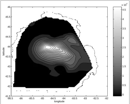
Figure 1.1: Gypsy moth counts in lower Michigan,1991

Figure 1.1 shows a contour of the moth counts for 1991 overlayed on a map outline of lower Michigan. We see the highest level of moth counts near Midland county Michigan in the center. As we move outward from the center,lower levels of moth counts occur taking the form of concentric rings. A set ofkdata points

(18)

each other. In terms of (1.1), yi and yj where both observationsiand j come

from the same ring should be highly correlated. The correlation of k1 points taken from one ring andk2 points from a neighboring ring should also exhibit a high correlation,but not as high as points sampled from the same ring. As we examine the correlation between points taken from more distant rings,we would expect the correlation to diminish.

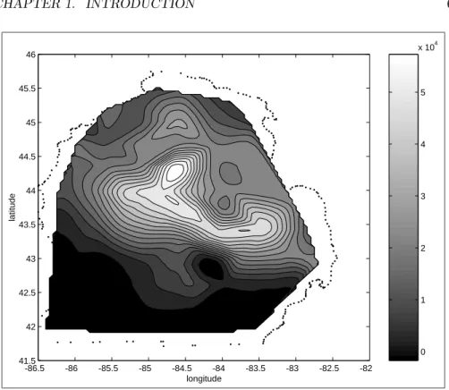
Over time the Gypsy moths spread to neighboring areas. They cannot fly,so the diffusion should be relatively slow. Figure 1.2 shows a similarly constructed contour map of moth counts for the next year,1992. We see some evidence of diffusion to neighboring areas between 1991 and 1992. The circular pattern of higher levels in the center and lower levels radiating out from the center is still quite evident.

-86.5 -86 -85.5 -85 -84.5 -84 -83.5 -83 -82.5 -82 41.5

42 42.5 43 43.5 44 44.5 45 45.5 46

longitude

latitude

0 1 2 3 4 5 6 x 104

(19)

-86.5 -86 -85.5 -85 -84.5 -84 -83.5 -83 -82.5 -82 41.5

42 42.5 43 43.5 44 44.5 45 45.5 46

longitude

latitude

0 1 2 3 4 5 x 104

How does this situation diﬀer from the traditional view of the process at work to generate economic data samples? The Gauss-Markov view of a regres-sion data sample is that the generating process takes the form of (1.2),where

y represent a vector ofn observations, X denotes an nxk matrix of explana-tory variables, β is a vector of k parameters and ε is a vector of n stochastic disturbance terms.

y=Xβ+ε (1.2)

The generating process is such that the X matrix and true parameters β are ﬁxed while repeated disturbance vectorsεwork to generate the samplesy that we observe. Given that the matrix X and parameters β are ﬁxed,the dis-tribution of sample y vectors will have the same variance-covariance structure as ε. Additional assumptions regarding the nature of the variance-covariance structure of ε were invoked by Gauss-Markov to ensure that the distribution of individual observations in y exhibit a constant variance as we move across observations,and zero covariance between the observations.

(20)

we move to observations from more distant rings.

Spatial dependence arising from underlying regional interactions in regional science data samples suggests the need to quantify and model the nature of the unspeciﬁed functional spatial dependence functionf(),set forth in (1.1). Before turning attention to this task,the next section discusses the other underlying condition leading to a need for spatial econometrics — spatial heterogeneity.

1.3Spatial heterogeneity

The term spatial heterogeneity refers to variation in relationships over space. In the most general case we might expect a diﬀerent relationship to hold for every point in space. Formally,we write a linear relationship depicting this as:

yi=Xiβi+εi (1.3)

Whereiindexes observations collected at i= 1, . . . , n points in space, Xi

rep-resents a (1 x k) vector of explanatory variables with an associated set of pa-rametersβi, yi is the dependent variable at observation (or location) i andεi

denotes a stochastic disturbance in the linear relationship.

A slightly more complicated way of expressing this notion is to allow the functionf() from (1.1) to vary with the observation indexi,that is:

yi=fi(Xiβi+εi) (1.4)

Restricting attention to the simpler formation in (1.3),we could not hope to estimate a set ofnparameter vectorsβigiven a sample ofndata observations.

We simply do not have enough sample data information with which to produce estimates for every point in space,a phenomena referred to as a “degrees of free-dom” problem. To proceed with the analysis we need to provide a specification for variation over space. This specification must be parsimonious,that is,only a handful of parameters can be used in the specification. A large amount of spatial econometric research centers on alternative parsimonious specifications for modeling variation over space. Questions arise regarding: 1) how sensitive the inferences are to a particular specification regarding spatial variation?,2) is the specification consistent with the sample data information?,3) how do competing specifications perform and what inferences do they provide?,and a host of other issues that will be explored in this text.

(21)

the restrictions are inconsistent with the sample data information?,and other issues we will explore.

One of the compelling motivations for the use of Bayesian methods in spatial econometrics is their ability to impose restrictions that are stochastic rather than exact in nature. Bayesian methods allow us to impose restrictions with varying amounts of prior uncertainty. In the limit,as we impose a restriction with a great deal of certainty,the restriction becomes exact. Carrying out our econometric analysis with varying amounts of prior uncertainty regarding a restriction allows us to provide a continuous mapping of the restriction’s impact on the estimation outcomes.

0 0.05 0.1 0.15 0.2 0.25 0.3 0.35 0.4

-5 0 5 10 15 20 25

Distance from CBD

distribution of homes

low-price mid-price high-price

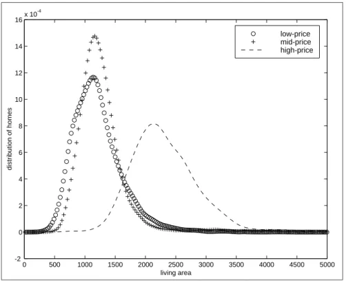
Figure 1.4: Distribution of low,medium and high priced homes versus distance

(22)

as they represent very high prices that are atypical.

Using the latitude-longitude coordinates,the distance from the central busi-ness district (CBD) in the city of Toledo,which is at the center of Lucas county was calculated. The three samples of 5,000 low, medium and high priced homes were used to estimate three empirical distributions that are graphed with respect to distance from the CBD in Figure 1.4.

We see three distinct distributions,with low-priced homes nearest to the CBD and high priced homes farthest away from the CBD. This suggests diﬀerent relationships may be at work to describe home prices in diﬀerent locations. Of course this is not surprising,numerous regional science theories exist to explain land usage patterns as a function of distance from the CBD. Nonetheless,these three distinct distributions provide a contrast to the Gauss-Markov assumption that the distribution of sample data exhibits a constant mean and variance as we move across the observations.

0 500 1000 1500 2000 2500 3000 3500 4000 4500 5000 -2

0 2 4 6 8 10 12 14 16x 10

-4

living area

distribution of homes

low-price mid-price high-price

Figure 1.5: Distribution of low,medium and high priced homes versus living area

(23)

priced homes have roughly similar distributions with regard to living space. It may be the case that important explanatory variables in the house value relationship change as we move over space. Living space may be unimportant in distinguishing between low and medium priced homes,but signiﬁcant for higher priced homes. Distance from the CBD on the other hand appears to work well in distinguishing all three categories of house values.

1.4 Quantifying location in our models

A ﬁrst task we must undertake before we can ask questions about spatial depen-dence and heterogeneity is quantiﬁcation of the locational aspects of our sample data. Given that we can always map a set of spatial data observations,we have two sources of information on which to draw.

The location in Cartesian space represented by latitude and longitude is one source of information. This information would also allow us to calculate dis-tances from any point in space,or the distance of observations located at distinct points in space to observations at other locations. Spatial dependence should conform to the fundamental theorem of regional science — distance matters. Observations that are near should reﬂect a greater degree of spatial dependence than those more distant from each other. This suggests the strength of spa-tial dependence between observations should decline with the distance between observations.

Distance might also be important for models involving spatially heteroge-neous relationships. If the relationship we are modeling varies over space,ob-servations that are near should exhibit similar relationships and those that are more distant may exhibit dissimilar relationships. In other words,the relation-ship may vary smoothly over space.

The second source of locational information is contiguity,reﬂecting the rel-ative position in space of one regional unit of observation to other such units. Measures of contiguity rely on a knowledge of the size and shape of the obser-vational units depicted on a map. From this,we can determine which units are neighbors (have borders that touch) or represent observational units in rea-sonable proximity to each other. Regarding spatial dependence,neighboring units should exhibit a higher degree of spatial dependence than units located far apart. For spatial heterogeneity,relationships may be similar for neighboring units.

It should be noted that these two types of information are not necessarily diﬀerent. Given the latitude-longitude coordinates of an observation,we can construct a contiguity structure by deﬁning a “neighboring observation” as one that lies within a certain distance. Consider also,given the boundary points associated with map regions,we can compute the centroid coordinates of the regions. These coordinates could then be used to calculate distances between the regions or observations.

(24)

contiguity,which is used in the models presented in Chapters 3 4 and 5. Chapters 6 and 7 deal with models that make direct use of the latitude-longitude coordinates,a subject discussed in the Section 1.4.2.

1.4.1 Quantifying spatial contiguity

Figure 1.6 shows a hypothetical example of five regions as they would appear on a map. We wish to construct a 5 by 5 binary matrixW containing 25 elements taking values of 0 or 1 that captures the notion of “connectiveness” between the five entities depicted in the map configuration. We record the contiguity relations for each region in the row of the matrixW. For example the matrix element in row 1,column 2 would record the presence (represented by a 1) or absence (denoted by 0) of a contiguity relationship between regions 1 and 2. As another example,the row 3,column 4 element would reflect the presence or absence of contiguity between regions 3 and 4. Of course,a matrix constructed in such fashion must be symmetric — if regions 3 and 4 are contiguous,so are regions 4 and 3.

It turns out there are a large number of ways to construct a matrix that contains contiguity information regarding the regions. Below,we enumerate some alternative ways to define a binary matrixW that reflects the “contiguity” relationships between the five entities in Figure 1.6. For the enumeration below, start with a matrix filled with zeros,then consider the following alternative ways to define the presence of a contiguity relationship.

Linear contiguity: DeﬁneWij = 1 for entities that share a common edge

to the immediate right or left of the region of interest. For row 1,where we record the relations associated with region 1,we would have allW1j =

0, j= 1, . . . ,5. On the other hand,for row 5,where we record relationships involving region 5,we would have W53 = 1 and all other row-elements

equal to zero.

Rook contiguity: Deﬁne Wij = 1 for regions that share a common side

with the region of interest. For row 1,reﬂecting region 1’s relations we would haveW12= 1 with all other row elements equal to zero. As another

example,row 3 would recordW34= 1, W35= 1 and all other row elements

equal to zero.

Bishop contiguity: DeﬁneWij= 1 for entities that share a common vertex

with the region of interest. For region 2 we would have W23= 1 and all

other row elements equal to zero.

Double linear contiguity: For two entities to the immediate right or left of the region of interest,deﬁneWij = 1. This deﬁnition would produce the

same results as linear contiguity for the regions in Figure 1.6.

Double rook contiguity: For two entities to the right,left,north and south of the region of interest deﬁne Wij = 1. This would result in the same

(25)

(1) (2)

(3)

(4)

(5)

Figure 1.6: An illustration of contiguity

Queen contiguity: For entities that share a common side or vertex with the region of interest deﬁneWij = 1. For region 3 we would have: W32=

1, W34= 1, W35= 1 and all other row elements zero.

(26)

The guiding principle is selecting a deﬁnition should be the nature of the problem being modeled,and perhaps additional non-sample information that is available. For example,suppose that a major highway connected regions (2) and (3) in Figure 1.6,and we knew that region (2) was a “bedroom community” for persons who work in region (3). Given this non-sample information,we would not rely on the rook deﬁnition because it rules out a contiguity relationship between these two regions.

We will use the rook definition to define a first-order contiguity matrix for the five regions in Figure 1.6 as a concrete illustration. This definition is often used in applied work. Perhaps the motivation for this is that we simply need to locate all regions on the map that have common borders with some positive length.

The matrix W in (1.5) shows ﬁrst-order rook’s contiguity relations for the ﬁve regions in Figure 1.6.

W =      

0 1 0 0 0

1 0 0 0 0

0 0 0 1 1

0 0 1 0 1

0 0 1 1 0

      (1.5)

Note thatW is symmetric,and by convention the matrix always has zeros on the main diagonal. A transformation often used in applied work converts the matrixW to have row-sums of unity. A standardized version of W from (1.5) is shown in (1.6).

C=      

0 1 0 0 0

1 0 0 0 0

0 0 0 1/2 1/2 0 0 1/2 0 1/2 0 0 1/2 1/2 0

      (1.6)

The motivation for the standardization can be seen by considering matrix multiplication ofCand a vector of observationsy ona variable associated with the ﬁve regions. This matrix product,y=Cy,represents a new variable equal to the mean of observations from contiguous regions as shown in (1.7).

      y 1 y₂ y₃ y4 y 5       =      

0 1 0 0 0

1 0 0 0 0

0 0 0 0.5 0.5 0 0 0.5 0 0.5 0 0 0.5 0.5 0

            y1 y2 y3 y4 y5             y 1 y 2 y 3 y 4 y 5       =       y2 y1

1/2y4+ 1/2y5

1/2y3+ 1/2y5

1/2y3+ 1/2y4

(27)

This is one way of quantifying the notion thatyi =f(yj), j=i,expressed

in (1.1). Equation (1.8) shows a linear relationship that uses the variabley

from (1.7) as an explanatory variable fory in a cross-sectional spatial sample of observations.

y=ρCy+ε (1.8)

The scalarρrepresents a regression parameter to be estimated andεdenotes the stochastic disturbance in the relationship. The parameterρ would reﬂect the spatial dependence inherent in our sample data,measuring the average inﬂuence of neighboring or contiguous observations on observations in the vector y. If we posit spatial dependence between the individual observations in the data sampley,some part of the total variation iny across the spatial sample would be explained by each observation’s dependence on its neighbors. The parameter

ρ would reﬂect this in the typical sense of regression. In addition,we could calculate the proportion of total variation inyexplained by spatial dependence using ˆρCy,where ˆρis the estimated value ofρ.

We will examine spatial econometric models that rely on this type of formu-lation in Chapter 3 where we set forth maximum likelihood estimation proce-dures for a taxonomy of these models known as spatial autoregressive models. Anselin (1988) provided this taxonomy and devised maximum likelihood meth-ods for producing estimates of these models. Chapter 4 provides a Bayesian approach to these models introduced by LeSage (1997) and Chapter 5 takes up limited dependent variable and censored data variants of these models from a Bayesian perspective that we introduce here. As this suggests,spatial autore-gressive models have historically occupied a central place in spatial econometrics and they are likely to play an important role in the future.

One point to note is that traditional explanatory variables of the type en-countered in regression can be added to the model in (1.8). We can represent these with the traditional matrix notation: Xβ,allowing us to modify (1.8) to take the form shown in (1.9).

y=ρCy+Xβ+ε (1.9)

Other extended speciﬁcations for these models will be taken up in Chapter 3.

1.4.2 Quantifying spatial position

(28)

and Chapter 7 where Bayesian variants are introduced. These models are also extended to the case of limited dependent variables.

Casetti (1972,1992) introduced one approach that involves a method he labels “spatial expansion”. The model is shown in (1.10),where y denotes an nx1 dependent variable vector associated with spatial observations and X

is annxnkmatrix consisting of terms xi representingkx1 explanatory variable

vectors,as shown in (1.11). The locational information is recorded in the matrix

Zwhich has elementsZxi, Zyi, i= 1, . . . , n,that represent latitude and longitude

coordinates of each observation as shown in (1.11).

The model posits that the parameters vary as a function of the latitude and longitude coordinates. The only parameters that need be estimated are the 2k

parameters inβ0that we denote,βx, βy. We note that the parameter vectorβin

(1.10) represents annkx1 vector in this model containing parameter estimates for allk explanatory variables at every observation.

y = Xβ+ε

β = ZJ β0 (1.10)

Where: y =      y1 y2 .. . yn      X =

    

x₁ 0 . . . 0

0 x₂

..

. . ..

0 x_n

     β=      β1 β2 .. . βn      ε=      ε1 ε2 .. . εn      Z =    

Zx1⊗Ik Zy1⊗Ik 0 . . .

0 . .. . ..

..

. Zxn⊗Ik Zyn⊗Ik

   J =

    

Ik 0

0 Ik

.. . 0 Ik

    

β0 =

βx

βy (1.11)

Recall that there is a need to achieve a parsimonious representation that introduces only a few additional parameters to be estimated. This approach accomplishes this task by conﬁning the estimated parameters to the 2kelements inβx, βy. This model can be estimated using least-squares to produce estimates

ofβxandβy. The remaining estimates for individual points in space are derived

using ˆβx and ˆβy in the second equation of (1.10). This process is referred to as

the “expansion process”. To see this,substitute the second equation in (1.10) into the ﬁrst,producing:

y=XZJ β0+ε (1.12)

(29)

This model would capture spatial heterogeneity by allowing variation in the underlying relationship such that clusters of nearby or neighboring observations measured by latitude-longitude coordinates take on similar parameter values. As the location varies,the regression relationship changes to accommodate a locally linear ﬁt through clusters of observations in close proximity to one another.

Another approach to modeling variation over space is based on the non-parametric locally linear regression literature from exploratory statistics dis-cussed in Becker,Chambers and Wilks (1988). In the spatial econometrics literature,McMillen (1996),McMillen and McDonald (1997) introduced these models and Brundson,Fotheringham and Charlton (1996) labeled these “geo-graphically weighted regression” (GWR) models.

These models use locally weighted regressions to produce estimates for every point in space based on sub-samples of data information from nearby observa-tions. Lety denote annx1 vector of dependent variable observations collected atn points in space, X annxk matrix of explanatory variables,andε annx1 vector of normally distributed,constant variance disturbances. LettingWi

rep-resent annxndiagonal matrix containing distance-based weights for observation

ithat reﬂects the distance between observationiand all other observations,we can write the GWR model as:

Wiy=WiXβi+εi (1.13)

The subscriptionβi indicates that thiskx1 parameter vector is associated

with observation i. The GWR model produces n such vectors of parameter estimates,one for each observation. These estimates are produced using least-squares regression on the sub-sample of observations as shown in (1.14).

ˆ

βi= (XWi2X)−1(XWi2y) (1.14)

One confusing aspect of this notation is that Wiy denotes an n-vector of

distance-weighted observations used to produce estimates for observationi. The notation is confusing because we usually rely on subscripts to index scalar mag-nitudes representing individual elements of a vector. Note also,thatWiX

repre-sents a distance-weighted data matrix,not a single observation andεirepresents

ann-vector.

The distance-based weights are speciﬁed as a decaying function of the dis-tance between observationiand all other observations as shown in (1.15).

Wi=f(θ, di) (1.15)

The vectordi contains distances between observationi and all other

obser-vations in the sample. The role of the parameter θ is to produce a decay of influence with distance. Changing the distance decay parameterθ results in a different weighting profile,which in turn produces estimates that vary more or less rapidly over space. Determination of the distance-decay parameterθusing cross-validation estimation methods is discussed in Chapter 5.

(30)

along with the distance information can be used to produce a set of parameter estimates for every point in the spatial data sample.

It may have occurred to the reader that a homogeneous model fit to a spatial data sample that exhibits heterogeneity will produce residuals that exhibit spa-tial dependence. The residuals or errors made by a homogeneous model fit to a heterogeneous relationship should reflect unexplained variation attributable to heterogeneity in the underlying relationship over space.

Spatial clustering of the residuals would occur with positive and negative residuals appearing in distinct regions and patterns on the map. This of course was our motivation and illustration of spatial dependence as illustrated in Fig-ure 1.1 showing the Gypsy moth counts in Michigan. You might infer correctly that spatial heterogeneity and dependence are often related in the context of modeling. An inappropriate model that fails to capture spatial heterogeneity will result in residuals that exhibit spatial dependence. This is another topic we discuss in this text.

1.4.3Spatial lags

A fundamental concept that relates to spatial contiguity is the notion of a spatial lag operator. Spatial lags are analogous to the backshift operatorB from time series analysis. This operator shifts observations back in time,where Byt =

yt−1,deﬁnes a ﬁrst-order lag andBpyt =yt−p represents a pth order lag. In

contrast to the time domain,spatial lag operators imply a shift over space but are restricted by some complications that arise when one tries to make analogies between the time and space domains.

Cressie (1991) points out that in the restrictive context of regular lattices or grids the spatial lag concept implies observations that are one or more distance units away from a given location,where distance units can be measured in two or four directions. In applied situations where observations are unlikely to represent a regular lattice or grid because they tend to be irregularly shaped map regions,the concept of a spatial lag relates to the set of neighbors associated with a particular location. The spatial lag operator works in this context to produce a weighted average of the neighboring observations.

In Section 1.4.1 we saw that the concept of “neighbors” in spatial analysis is not unambiguous,it depends on the deﬁnition used. By analogy to time se-ries analysis it seems reasonable to simply raise our ﬁrst-order binary contiguity matrixW containing 0 and 1 values to a power,say pto create a spatial lag. However,Blommestein (1985) points out that doing this produces circular or redundant routes,where he draws an analogy between binary contiguity and the graph theory notion of an adjacency matrix. If we use spatial lag matrices pro-duced in this way in maximum likelihood estimation methods,spurious results can arise because of the circular or redundant routes created by this simplistic approach. Anselin and Smirnov (1994) provide details on many of the issues involved here.

(31)

0 5 10 15 20 25 30 35 40 45 50 0

5

10

15

20

25

30

35

40

45

50

nz = 232

Figure 1.7: First-order spatial contiguity for 49 neighborhoods

weight matrices representing higher-order contiguity relationships. The spatial econometrics library contains a function to properly construct spatial lags of any order and the function deals with eliminating redundancies.

We provide a brief illustration of how spatial lags introduce information regarding “neighbors to neighbors” into our analysis. These spatial lags will be used in Chapter 3 when we discuss spatial autoregressive models.

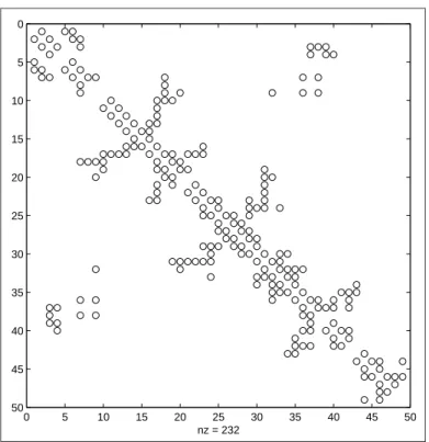
To illustrate these ideas,we use a ﬁrst-order contiguity matrix for a small data sample containing 49 neighborhoods in Columbus,Ohio taken from Anselin (1988). This contiguity matrix is typical of those encountered in applied prac-tice as it relates irregularly shaped regions representing each neighborhood. Figure 1.7 shows the pattern of 0 and 1 values in a 49 by 49 grid. Recall that a non-zero entry in rowi,column j denotes that neighborhoods i and j

have borders that touch which we refer to as “neighbors”. Of the 2401 possible elements in the 49 by 49 matrix,there are only 232 are non-zero elements des-ignated on the axis in the figure by ‘nz = 232’. These non-zero entries reflect the contiguity relations between the neighborhoods. The first-order contiguity matrix is symmetric which can be seen in the figure. This reflects the fact that if neighborhoodibordersj,thenj must also borderi.

(32)

0 5 10 15 20 25 30 35 40 45 50 0

5

10

15

20

25

30

35

40

45

50

nz = 410

Figure 1.8: A second-order spatial lag matrix

second-order spatially lagged matrix,whose non-zero elements are represented by a ‘+’ symbol in the ﬁgure. This graphical depiction of a spatial lag demon-strates that the spatial lag concept works to produce a contiguity or connective-ness structure that represents “neighbors of neighbors”.

How might the notion of a spatial lag be useful in spatial econometric model-ing? We might encounter a process where spatial diffusion effects are operating through time. Over time the initial impacts on neighbors work to influence more and more regions. The spreading impact might reasonably be considered to flow outward from neighbor to neighbor,and the spatial lag concept would capture this idea.

As an illustration of the redundancies produced by simply raising a first-order contiguity matrix to a higher power,Figure 1.9 shows a second-order spatial lag matrix created by simply powering the first-order matrix. The non-zero elements in this inappropriately generated spatial lag matrix are represented by ‘+’ symbols with the original first-order non-zero elements denoted by ‘o’ symbols. We see that this second order spatial lag matrix contains 689 non-zero elements in contrast to only 410 for the correctly generated second order spatial lag matrix that eliminates the redundancies.

(33)

au-0 5 10 15 20 25 30 35 40 45 50 0

5

10

15

20

25

30

35

40

45

50

nz = 689

Figure 1.9: A contiguity matrix raised to a power 2

toregressive models in Chapters 3,4 and 5. The MATLAB function from the spatial econometrics library as well as other functions for working with spatial contiguity matrices will be presented along with examples of their use in spatial econometric modeling.

1.5 Chapter Summary

This chapter introduced two main features of spatial econometric relationships, spatial dependence and spatial heterogeneity. Spatial dependence refers to the fact that sample data observations exhibit within-sample correlation with ref-erence to the location of the sample observations in space. We often observe spatial clustering of sample data observations with respect to map regions. An intuitive motivation for this type of result is the existence of spatial hierarchical relationships,spatial spillovers and other types of spatial interactivity studied in regional science.

(34)

the estimated relationship to vary systematically over space. These methods attempt to achieve a parsimonious speciﬁcation of systematic variation in the relationship such that only a few additional parameters need be estimated.

A large part of the chapter was devoted to introducing how locational infor-mation regarding sample data observations is formally incorporated in spatial econometric models. After introducing the concept of a spatial contiguity ma-trix,we provided a preview of spatial autoregressive models that rely on the contiguity concept. Chapters 3,and 4 cover this spatial econometric method in detail,and Chapter 5 extends this model to cases where the sample data represent limited dependent variables or variables subject to censoring.

(35)

Chapter 2

The MATLAB spatial

econometrics library

As indicated in the preface to this text,all of the spatial econometric methods discussed in the text have been implemented using MATLAB software from the MathWorks Inc. All readers should read this chapter as it provides an intro-duction to the design philosophy that should be helpful to anyone using the functions. A consistent design was implemented that provides documentation, example programs,and functions to produce printed as well as graphical pre-sentation of estimation results for all of the econometric functions. This was accomplished using the “structure variables” introduced in MATLAB Version 5. Information from econometric estimation is encapsulated into a single vari-able that contains “ﬁelds” for individual parameters and statistics related to the econometric results. A thoughtful design by the MathWorks allows these structure variables to contain scalar,vector,matrix,string,and even multi-dimensional matrices as ﬁelds. This allows the econometric functions to return a single structure that contains all estimation results. These structures can be passed to other functions that can intelligently decipher the information and provide a printed or graphical presentation of the results.

In Chapter 3 we will see our first example of constructing MATLAB functions to carry out spatial econometric estimation methods. Here,we discuss some design issues that affect all of the spatial econometric estimation functions and their use in the MATLAB software environment. The last section in this chapter discusses sparse matrices and functions that are used in the spatial econometrics library to achieve fast and efficient solutions for large problems with a minimum of computer memory.

2.1 Structure variables in MATLAB

In designing a spatial econometric library of functions,we need to think about organizing our functions to present a consistent user-interface that packages

(36)

all of our MATLAB functions in a uniﬁed way. The advent of ‘structures’ in MATLAB version 5 allows us to create a host of alternative spatial econometric functions that return ‘results structures’.

A structure in MATLAB allows the programmer to create a variable con-taining what MATLAB calls ‘ﬁelds’ that can be accessed by referencing the structure name plus a period and the ﬁeld name. For example,suppose we have a MATLAB function to perform ordinary least-squares estimation named ols that returns a structure. The user can call the function with input arguments (a dependent variable vectory and explanatory variables matrixx) and provide a variable name for the structure that theolsfunction will return using:

result = ols(y,x);

The structure variable ‘result’ returned by ourolsfunction might have fields named ‘rsqr’,‘tstat’,‘beta’,etc. These fields would contain the R-squared statistic,t−statistics for the ˆβ estimates and the least-squares estimates ˆβ. One virtue of using the structure to return regression results is that the user can access individual fields in the structure that may be of interest as follows:

bhat = result.beta; disp(‘The R-squared is:’); result.rsqr

disp(‘The 2nd t-statisticis:’); result.tstat(2,1)

There is nothing sacred about the name ‘result’ used for the returned struc-ture in the above example,we could have used:

bill_clinton = ols(y,x); result2 = ols(y,x); restricted = ols(y,x); unrestricted = ols(y,x);

That is,the name of the structure to which theols function returns its infor-mation is assigned by the user when calling the function.

To examine the nature of the structure in the variable ‘result’,we can sim-ply type the structure name without a semi-colon and MATLAB will present information about the structure variable as follows:

result = meth: ’ols’

y: [100x1 double] nobs: 100.00

nvar: 3.00

beta: [ 3x1 double] yhat: [100x1 double] resid: [100x1 double]

sige: 1.01

tstat: [ 3x1 double] rsqr: 0.74

(37)

Each field of the structure is indicated,and for scalar components the value of the field is displayed. In the example above,‘nobs’,‘nvar’,‘sige’,‘rsqr’, ‘rbar’,and ‘dw’ are scalar fields,so there values are displayed. Matrix or vector fields are not displayed,but the size and type of the matrix or vector field is indicated. Scalar string arguments are displayed as illustrated by the ‘meth’ field which contains the string ‘ols’ indicating the regression method that was used to produce the structure. The contents of vector or matrix strings would not be displayed,just their size and type. Matrix and vector fields of the structure can be displayed or accessed using the MATLAB conventions of typing the matrix or vector name without a semi-colon. For example,

result.resid result.y

would display the residual vector and the dependent variable vector y in the MATLAB command window.

Another virtue of using ‘structures’ to return results from our regression functions is that we can pass these structures to another related function that would print or plot the regression results. These related functions can query the structure they receive and intelligently decipher the ‘meth’ ﬁeld to determine what type of regression results are being printed or plotted. For example,we could have a functionprt that prints regression results and another plt that plots actual versus ﬁtted and/or residuals. Both these functions take a structure returned by a regression function as input arguments. Example 2.1 provides a concrete illustration of these ideas.

The example assumes the existence of functions ols, prt, plt and data matricesy, xin ﬁles ‘y.data’ and ‘x.data’. Given these,we carry out a regression, print results and plot the actual versus predicted as well as residuals with the MATLAB code shown in example 2.1. We will discuss theprtandpltfunctions in Section 2.2.

% --- Example 1.1 Demonstrate regression using the ols() function load y.data;

load x.data; result = ols(y,x); prt(result); plt(result);

2.2 Constructing estimation functions

Now to put these ideas into practice,consider implementing an ols function. The function code would be stored in a ﬁle ‘ols.m’ whose ﬁrst line is:

function results=ols(y,x)

(38)

The help portion of the MATLAB ‘ols’ function is presented below and fol-lows immediately after the ﬁrst line as shown. All lines containing the MATLAB comment symbol ‘%’ will be displayed in the MATLAB command window when the user types ‘help ols’.

function results=ols(y,x)

% PURPOSE: least-squares regression

%---% USAGE: results = ols(y,x)

% where: y = dependent variable vector (nobs x 1) % x = independent variables matrix (nobs x nvar) %---% RETURNS: a structure

% results.meth = ’ols’ % results.beta = bhat % results.tstat = t-stats % results.yhat = yhat % results.resid = residuals % results.sige = e’*e/(n-k) % results.rsqr = rsquared % results.rbar = rbar-squared

% results.dw = Durbin-Watson Statistic % results.nobs = nobs

% results.nvar = nvars

% results.y = y data vector

% ---% SEE ALSO: prt(results), plt(results)

%---if (nargin ~= 2); error(’Wrong # of arguments to ols’); else

[nobs nvar] = size(x); nobs2 = length(y);

if (nobs ~= nobs2); error(’x and y not the same # obs in ols’); end; end;

results.meth = ’ols’; results.y = y; results.nobs = nobs; results.nvar = nvar; [q r] = qr(x,0); xpxi = (r’*r)\eye(nvar); results.beta = xpxi*(x’*y);

results.yhat = x*results.beta; results.resid = y - results.yhat; sigu = results.resid’*results.resid; results.sige = sigu/(nobs-nvar); tmp = (results.sige)*(diag(xpxi));

results.tstat = results.beta./(sqrt(tmp)); ym = y - mean(y);

rsqr1 = sigu; rsqr2 = ym’*ym;

results.rsqr = 1.0 - rsqr1/rsqr2; % r-squared rsqr1 = rsqr1/(nobs-nvar); rsqr2 = rsqr2/(nobs-1.0); results.rbar = 1 - (rsqr1/rsqr2); % rbar-squared

ediff = results.resid(2:nobs) - results.resid(1:nobs-1); results.dw = (ediff’*ediff)/sigu; % durbin-watson

(39)

The ‘USAGE’ section describes how the function is used,with each input argument enumerated along with any default values. A ‘RETURNS’ section portrays the structure that is returned by the function and each of its fields. To keep the help information uncluttered,we assume some knowledge on the part of the user. For example,we assume the user realizes that the ‘.residuals’ field would be an (nobs x 1) vector and the ‘.beta’ field would consist of an (nvar x 1) vector.

The ‘SEE ALSO’ section points the user to related routines that may be use-ful. In the case of ourolsfunction,the user might what to rely on the printing or plotting routinesprt andplt,so these are indicated. The ‘REFERENCES’ section would be used to provide a literature reference (for the case of our more exotic spatial estimation procedures) where the user could read about the de-tails of the estimation methodology. The ‘NOTES’ section usually contains important warnings or requirements for using the function. For example,some functions in the spatial econometrics library require that if the model includes a constant term,the ﬁrst column of the data matrix should contain the constant term vector of ones. This information would be set forth in the ‘NOTES’ sec-tion. Other uses of this section would be to indicate that certain optional input arguments are mutually exclusive and should not be used together.

As an illustration of the consistency in documentation,consider the func-tion sar that provides estimates for the spatial autoregressive model that we presented in Section 1.4.1. The documentation for this function is shown below. It would be printed to the MATLAB command window if the user typed ‘help sar’ in the command window.

PURPOSE: computes spatial autoregressive model estimates y = p*W*y + X*b + e, using sparse matrix algorithms

---USAGE: results = sar(y,x,W,rmin,rmax,convg,maxit) where: y = dependent variable vector

x = explanatory variables matrix W = standardized contiguity matrix

rmin = (optional) minimum value of rho to use in search rmax = (optional) maximum value of rho to use in search convg = (optional) convergence criterion (default = 1e-8) maxit = (optional) maximum # of iterations (default = 500)

---RETURNS: a structure

results.meth = ’sar’ results.beta = bhat results.rho = rho

results.tstat = asymp t-stat (last entry is rho) results.yhat = yhat

results.resid = residuals

results.sige = sige = (y-p*W*y-x*b)’*(y-p*W*y-x*b)/n results.rsqr = rsquared

results.rbar = rbar-squared results.lik = -log likelihood results.nobs = # of observations

results.nvar = # of explanatory variables in x results.y = y data vector