Serie documentos de trabajo
Family Income Inequality and the Role of Married Females' Earnings in Mexico: 1988-2010
Raymundo M. Campos Vázquez El Colegio de México
Andres Hincapie
Washington University in St. Louis
Ruben Irvin Rojas-Valdes
El Colegio de México
Abril, 2012
1
Family Income Inequality and the Role of Married Females' Earnings in
Mexico: 1988-2010
♠Raymundo M. Campos-Vazquez *
Centro de Estudios Económicos, El Colegio de México, Mexico City, Mexico.
Andres Hincapie +
Ph. D. Student, Department of Economics, Washington University in St. Louis, St. Louis, USA.
Ruben Irvin Rojas-Valdes ¤
Centro de Estudios Económicos, El Colegio de México, Mexico City, Mexico.
Abstract
We study family income inequality in Mexico from 1988 to 2010. The share of married females' income
among married couples grew from 13 to 23 percent in the period. However, the correlation of married
males' and married females' earnings has been fairly stable at 0.28, one of the highest correlations
recorded across countries. We follow Cancian and Reed's (1999) methodology in order to analize
whether married females' income equalizes total family income distribution. We investigate several
counterfactuals and conclude that the increment in female employment has contributed to a decrease in
family income inequality through a rise in married females' labor supply in poor families.
Keywords: Income Inequality; Female Employment; Female Earnings; Latin America; Mexico.
JEL Codes: J12; J21; J31; O15; O54.
♠
This is a forthcoming article in “Latin American Journal of Economics”. It will be published in May or August 2012. A previous version of the article was titled “Family Income Inequality and the Role of Wives’ Earnings in Mexico: 1988-2010”. We thank Eva O. Arceo-Gómez, James Cameron, Gerardo Esquivel, Anna Isaykina, Julia Rozanova, Isidro Soloaga and Christopher Wildeman for valuable comments. We especially thank an anonymous referee for precise comments and suggestions. All remaining errors are our own. Andres Hincapie acknowledges financial support from the Fox International Fellowship at Yale University.
*
Address: El Colegio de México, Centro de Estudios Económicos, Camino al Ajusco 20, Pedregal de Santa Teresa, 10740, México, DF. E-mail: [email protected]. Website: http://raycampos.googlepages.com. Phone: +52-55-54493000, ext. 4153. Fax: +52-55-56450464.
+
Address: One Brookings Drive, 63130, St. Louis, MO. E-mail: [email protected]. Phone: +1-314-9355670.
¤
2 1. Introduction
Latin America is characterized by being a highly unequal region in terms of income (Ferreira et al., 2003; Lopez and Perry, 2008). Mexico is also characterized by large income
inequality: Gini coefficient computations yield a figure around 0.52 in 2005, the 15th highest of 24 countries in Latin America with comparable data (Lopez and Perry, 2008; Lopez-Calva and Lustig, 2010).1 However, since the mid 1980s Mexico has seen two different trends of inequality. From the mid 1980s to the mid 1990s inequality in Mexico increased (Cragg and Epelbaum, 1996; Esquivel and Rodrguez-López, 2003). But since the mid to late 1990s there has been a decline in labor income inequality (Esquivel, 2009; Esquivel, Lustig and Scott, 2010; Robertson, 2007). At the same time, female labor force participation has increased substantially, especially for low skilled female workers. For example, from 1996-2010 female labor force participation increased 11 percentage points.2 Among females, married females increased their labor participation the most.
We investigate the effects of this recent increase in female labor supply among married females and their earnings on the distribution of family income. Family income is not only widely used as a measure of income inequality in the literature (see Cancian and Reed, 1998, 1999; Amin and DaVanzo, 2004; Gottschalk and Danziger, 2005), it also allows us to capture characteristics that are of special interest for policy makers. For example, an analysis of family income allows to account for the correlation of earnings among spouses or among members in the household, as well as to account for changes in the income contribution to total income by each member in the household. The goal of the paper is then to analize whether married females' earnings in married-couple households and the change in marriage
1
The Gini coefficient in Mexico for 2008 is 0.506 according to the Mexican institute in charge of measuring official poverty. See National Council for the Evaluation of Social Development Policy (CONEVAL), http://www.coneval.gob.mx.
2
3
rates have an equalizing effect on the family income distribution. In particular, we simulate the level of inequality that would have existed under different scenarios.
There are two commonly used methods to deconstruct changes in family income distribution that assess the effect of an increase in married females' earnings on family income inequality. A semiparametric method has been used to analyze changes in observable characteristics of the family (DiNardo et. al., 1996; Machado and Mata, 2005). The other, which we employ here, is based on decomposing the coefficient of variation in a fashion that separates the contribution of each income source (Cancian and Reed, 1998, 1999; Del Boca and Pasqua, 2003; Amin and DaVanzo, 2004).
4
households. We study the effects of married females' earnings on family income for married-couple households and for the whole population. We estimate family income inequality using equivalence scales under different scenarios for the two broad groups mentioned above. First, we calculate inequality trends at the individual and household level and show that it follows an inverted U-shape pattern. Then we simulate the effects of married males’ earnings and married females’ earnings and the correlation of earnigs among spouses on the family income distribution. In particular, we ask what would have happened had each component kept constant at its 1988 level. Three main findings emerge from this exercise. First, males’ earnings are the main determinant of family inequality given that their share of income within the family is high. Second, the change in married female labor supply
contributes to a decline in family income inequality, especially in the last decade. Finally, the correlation of earnings among spouses does not explain changes in family income inequality.
Also, we analyze the effects of changes in marriage rates on inequality. We find that had marriage rates kept constant at the 1988 level, inequality would have been lower. In sum, even though we notice an increase in female labor supply for all groups, it is particularly higher for married females, low-skilled females and especially for married females in poor families. We also find that the correlation between married males' and married females' earnings has been fairly stable over time. Furthermore, its value, of about 0.28, is among the highest correlations recorded across developed countries (Pasqua, 2008). Hence, family income inequality did not fall because of a reduction in income assortative mating, its decrease is driven by the increase in married females' labor supply for poor households and also by changes in wage inequality within married females.
5
Since we only account for the effect of married females’ earnings on family income inequality, we cannot make behavioral interpretations of the responses of other income sources within the framework proposed. Also, we do not attempt to calculate the role of household structure on family income inequality.
The paper is structured as follows. In section 2, we review previous findings on whether females contribute to equalize the income distribution. Section 3 discusses the methodology proposed by Cancian and Reed (1999) and explains the counterfactuals we use. Section 4 introduces the data as well as some descriptive results. Section 5 presents the main results of the paper. In section 6 we briefly explore possible channels of transmission between female labor supply and family income inequality. Finally, we conclude in section 7.
2. Literature Review
Social sciences academics have been widely interested in the dynamics of income inequality and its potential causes. Particularly, the study of wage inequality has been of special interest among labor economists.3 For the period 1988-2010 in Mexico, income and wage inequality follow an inverted-U-shape pattern (Lopez-Calva and Lustig, 2010, and Esquivel, Lustig and Scott, 2010). There has been a substantial number of studies that analyze the potential causes of change in inequality at the individual level.4 However, little is known about the role of
3 Katz and Autor (1999) and Machin (2008) present a general review of the findings regarding the sources of change in
wage inequality. For the U.S. the consensus is that both competitive and non-competitive sources are responsible for changes in the wage distribution. For example, relative wages can change due to supply and demand (competitive factors) but also through changes in the minimum wages and unionization rates.
4
6
married females' earnings on the distribution of family incomein Mexico.
The distribution of family income is also an important topic to study. In general, we observe an increase in female labor force participation across countries over time. The rise in family earnings due to married females labor supply decision may increase or decrease family income inequality depending on the evolution of married males' income and also depending on whether married females in poor or rich families augmented their participation the most. While inequality at the individual level may decrease, the effects on family income inequality may not be of the same magnitude or even move in the opposite way. For instance, Juhn and Murphy (1997) study the period 1969-1989 in the U.S. and find that female employment and earnings have increased the most for females married to high income males. This change suggests a process of assortative mating and an increase in family income inequality due to this process. Nevertheless, Juhn and Murphy (1997) do not analyze the consequences on family income inequality. Gottschalk and Danziger (2005) document changes in inequality for the period 1975-2002 in the U.S. showing that male wage inequality and family income inequality move in general in the same way. They argue that inequality would have increased by more than it did had other members in the household not increased their hours of work. This suggests that the increase in female labor force participation offsets the effect of increasing male wage inequality in the U.S. However, Gottschalk and Danziger (2005) do not use any decomposition method to further investigate their claims.
There are two commonly used methods to decompose changes in family income distribution. While in the first one an inequality index is decomposed, a semiparametric procedure is used to analyze changes in observable characteristics in the second method (DiNardo et. al., 1996; Machado and Mata, 2005). Cancian and Reed (1998, 1999)
7
on the distribution of family income. They use the Current Population Surveys (CPS) in the U.S. for the period 1968-1995 and conclude that changes in married females' labor supply and married females' earnings have caused a decline in family income inequality. Following a similar methodology, but using a longitudinal dataset, Lehrer (2000) confirms the findings in Cancian and Reed (1998, 1999). Following DiNardo, Fortin and Lemieux (1996), Daly and Valleta (2006) find that, on the one hand, family income inequality has decreased due to female earnings but, on the other, it has increased due to changes in family structure such as marital status and number of children.5 In sum, different studies for the U.S. case conclude that married females' earnings reduce family income inequality.
Similar results have been found for the case of Italy and the U.K. Del Boca and Pasqua (2003), using a coefficient-of-variation decomposition for the period 1977-1998 in Italy, conclude that married females' earnings have an equalizing effect on the family income distribution. For the period 1968-1990 in the U.K., Davies and Joshi (1998) show that female labor force participation had a small equalizing effect but created a gap between employed- and not-employed-wife households. Using cross-country analysis for developed countries, Pasqua (2008) and Harkness (2010) show that, in general, female earnings reduce family income inequality.
However, in studies for other countries, researchers have found different results. For example, Johnson and Wilkins (2004) analyze the case of Australia in the period 1982-1998 using a semiparametric decomposition. Although they conclude that changes in the labor force status of the households' members increased family income inequality, they do not differentiate between wife labor force status and other-household-members status. Aslaksen,
5
8
Wennemo, and Aaberge (2005) analyze the case of Norway for the period 1973-1997 and find a disequalizing effect of female labor income among married couples. They conclude that this process is due to a flocking together effect, or an increase in assortative mating. For the case of Brazil 1977-2007, Sotomayor (2009) finds that female earnings do not affect the distribution of income in general terms, but they do play an important role in decreasing poverty rates. Evidence of the role of female earnings on family income inequality is limited for developing countries. In particular, little is known about the role of married females' earnings in the distribution of family income in Mexico.6
Given the lack of evidence for developing countries and especially for Mexico, the analysis of the role of married females' earnings in family income inequality is particularly relevant. Our paper contributes to the literature in at least two different ways. First, we provide descriptive analysis on the patterns of marriage rates, family income inequality and female labor supply patterns. Second, we formally analyze the role of married females' earnings on inequality using the methods described by Cancian and Reed (1998, 1999) and compare the results to other studies in different countries.
3. Implementation
We follow Cancian and Reed (1998, 1999) in order to estimate the effect of married females' earnings on family income inequality. We divide families into two broad groups according to the household head status: married-couple families, those in which both partners, legally married or not, live together (group A); and all the other families, including married individuals whose partner does not currently live in the household, single, divorced and
6
9
widowed individuals (group B). We include the second group in order to analyze the effect of changing marriage rates on the family income distribution. Married-couple family income can be decomposed into three sources: husband income, wife income, and residual income. For group B, we only aggregate income at the family level.
Different indexes of inequality are employed in the literature. Among those, we use the coefficient of variation (CV ) to analyze the role of married females' earnings on family income inequality.7 As pointed out by Cancian and Reed (1998, 1999), the CV can be decomposed into different sources. A useful decomposition for married-couple families is the following:
𝐶𝑉𝐴2 =𝑆𝑚2𝐶𝑉𝑚2 +𝑆𝑤2𝐶𝑉𝑤2+𝑆𝑜2𝐶𝑉𝑜2+ 2𝜌𝑚𝑤𝑆𝑚𝑆𝑤𝐶𝑉𝑚𝐶𝑉𝑤
+2𝜌𝑚𝑜𝑆𝑚𝑆𝑜𝐶𝑉𝑚𝐶𝑉𝑜+ 2𝜌𝑤𝑜𝑆𝑜𝑆𝑤𝐶𝑉𝑜𝐶𝑉𝑤 (1)
where
ho hw hm
hi i
Y Y Y
Y S
+ +
= is the share of income (Yh) in household h for married males (
m), married females (w) and other sources (o), and i=m,w,o. CVi is the coefficient of variation for each group and ρij is the correlation coefficient between income source i and
j.8 CVA denotes the coefficient of variation for married couples.
Equation (1) refers to only married-couple households. We use an additional
7
Even though the Gini coefficient may be decomposed into different sources as well, its main disadvantage is that it is not additive across groups, that is, total Gini of a group is not equal to the sum of the Ginis for its subgroups (Cancian and Reed, 1998, 1999). Cancian and Reed (1998, p. 74) provide an excellent example to clarify the point: “Consider the hypothetical situation in which wives' earnings are equal across all married couples. In the absence of wives' earnings, the distribution of family income would become less equal... However, the Gini contribution of wives' earnings to family income inequality is zero.”
8
10
decomposition for the CV in order to include all families in the sample. If we have two broad groups (married-couple families and other families), the CV in the sample is given by
𝐶𝑉2 = 𝜇 𝐴�𝑌����𝑌�𝐴�
2
𝐶𝑉𝐴2+𝜇𝐵�𝑌����𝑌�𝐵� 2
𝐶𝑉𝐵2+�𝜇𝐴�𝑌����𝑌�𝐴� 2
+𝜇𝐵�����𝑌𝑌�𝐵� 2
�/𝑌� (2)
where µ is the proportion of families in each group, and Y is the group's average income. Hence, it is possible to calculate the contribution of each component and create
counterfactual trends of what would have happened had one component behaved differently. For example, parameter
µ
B measures the percentage of all families but married-couple families. In the last 20 years, the percent of married-couple families has decreased in Mexico. We can ask, then, what would have happened to family income inequality had marriage rate kept constant at its 1988 level. This counterfactual is easily created by keeping constantµ
B for every year in the calculation.The focus of our paper is on estimating the effect of married females’ earnings on family income inequality. In particular, our purpose is to address how the level of family income inequality would have changed if the participation of women in the labor force and their earnings had been different.
The main insight in Cancian and Reed (1998, 1999) is that we can create many
11
parameters move freely, we can observe whether that parameter increases or reduces family income inequality. We calculate:9
(1) What would have happened to family income inequality if all variables in equation (1) had remained constant at their 1988 levels except inequality among married males? In other words, we fix all parameters in equation (1) except 𝐶𝑉𝑚2. This counterfactual provides the contribution of married males to total inequality.
(2) What would have happened to family income inequality if all variables in equation (1) had remained constant at their 1988 levels except inequality among married males and females? In this counterfactual we can vary either 𝑆𝑤2 or 𝐶𝑉𝑤2. Assume we let 𝑆𝑤2 to vary and set 𝐶𝑉𝑤2 constant at its 1988 level (as well as the rest of the variables). In this case, and in order to provide some intuition, assume the share of income of married females increases. Hence, the counterfactual assumes that the same type of women that were working in 1988 work in each period but receive a larger income share. If women from poor families were to increase their labor supply, the formula in equation (1) would not take that into account. In this way, fixing 𝐶𝑉𝑤2 and varying 𝑆𝑤2 provides the effect of higher income to the “same women” that were participating in 1988, and it does not provide the effect of an increase in female labor supply of different types of families. On the other hand, if 𝐶𝑉𝑤2 is allowed to vary, then we are calculating the effect of the female wage structure on family income inequality. In general, a change in female labor force participation may affect both the share of income and inequality. From the previous discussion, the problem of separating an increase in female labor force participation from both 𝑆𝑤2 and 𝐶𝑉𝑤2 is clear. In practice, we calculate the contribution of each component
9
12
separately and combined.
(3) If in addition to counterfactual (2) we let the correlation of earnings change as it did, what would have happened to inequality? This counterfactual provides the relative importance of the correlation parameters in equation (1). If income assortative mating is an important contributor to family inequality, then we should observe a difference in inequality between this counterfactual and observed inequality. For example, if income assortative mating increases from 1988 to 2010, inequality should be lower over the period when fixing the correlation parameter to its 1988 level.
(4) Finally, what would have happened to inequality if the percent of married-couple households had not changed over time? In this counterfactual, we explore the role of marriage rates using equation (2).
One disadvantage of the decomposition we have just discussed is that the results are sensitive to the ordering of the parameters that determine inequality. In other words, the contribution of each component to total inequality depends on the ordering we choose. In order to solve this problem, we calculate the contribution of each component using all possible orderings and then take the average contribution of each component. We focus on three main components: (a) married males inequality, (b) married females’ share of income and inequality, and (c) correlation of earnings within the family. As we have three main components, we have six possible orderings which we calculate to determine the average contribution of each of them.
4. Data and Descriptive Statistics
13
(INEGI).10 In particular, we use the following labor force surveys for the urban sector: the Encuesta Nacional de Empleo Urbano, 1987-1994; the Encuesta Nacional de Empleo, 1995-2004; and the Encuesta Nacional de Ocupación y Empleo, 2005-2010.11 Although some questions of the survey change from one survey to other, socioeconomic variables, such as age, education, marital status, monthly labor income and weekly working hours are always comparable. In each survey, information regarding all household members is recorded. We refer to all surveys as the labor force surveys.12,13
According to INEGI, a household is a group of one or more people living in a house sharing expenses (individuals in the household may or may not be relatives). Following Cancian and Reed (1999), the unit of analysis is the family, not the household that is interviewed. Hence, we employ a different definition of household in order to isolate
household members who are not relatives of the household head. We define a new household code to account for those individuals and consider them as an individual household.14
In order to derive some descriptive statistics, we focus on four main samples of families. First, we consider married couples, their children, and other relatives living in the same household. This group is comparable with the sample of married couples in Cancian and Reed (1998, 1999). For each household, we compute the family income as the sum of all family members' labor income. We identify married males' income, married females' income
10 Data are available at http://www.inegi.org.mx.
11
Surveys contain registers for over 100,000 households, which is especially useful given the number of different categories we use in the paper. We use only the second quarter because ENE is national representative only for that quarter. We use only the urban sector (defined as municipalities with more than 100,000 inhabitants) because ENEU is by definition an urban survey. So, in order to cover the longest period in the analysis, our sample limits to the urban segment (between 40 and 50 percent of the whole population) in the second quarter of each year. These surveys are comparable in general to the ones carried out by the CPS.
12
Another survey traditionally used for Mexico is the Household Expenditure-Income Survey (ENIGH). However, ENIGH is not available every year since 1988, and the sample sizes are considerably lower.
13
Although we present the main results for the urban sample starting in 1988, we also estimate the results (not reported) using the national sample starting in 1995. Results are similar for both samples.
14
14
and other sources' income.
Instead of analysing the rest of the population as one single group, we define three groups of families in order to understand which of them are non-married-couple families. Firstly, we broaden the definition of household of the original survey to include single headed households, their children and relatives living in the household. Secondly, we define a group that consists of those heads who declare to be married or cohabitating but whose spouses do not live in the household (plus their children and relatives). The final group consists of those people living alone (singles, divorced, separated and widows) or that are not relatives of the household head. We consider each of those groups a single family. For these households, we only compute the total family income since there is no spouse present. In order to avoid outliers with the income measure, we follow the standard literature on wages and trim labor income to the 0.05 and 99.5 percentiles respectively. Income is adjusted for inflation and expressed in January 2010 pesos.
We drop those individuals whose relationship with the household head is not specified and those with missing information about their education, age, marital status, and household head status. We also drop all households (and their members) that declare more than one head or more than one spouse.15 Additionally, we only keep households in which the head is at least 18 years old and less than 65 years old. Finally, we only use information on
households in which at least one of its members reports positive income. Although zero income households may depend on non-monetary income, the focus of our paper is on the effect of labor income on labor income inequality. Furthermore, the inclusion of these dropped households does not affect our results.
Comparing total income across all families may be inadequate due to family size scale
15
15
effects. Most of the studies that deal with family income use a general equivalence scale to adjust for family size. Since the equivalence scale used in studies for other countries may not be suited for a developing country like Mexico, we use the equivalence scale published by the National Council for the Evaluation of Social Development Policy (CONEVAL).16 The equivalence scale gives a weight of 0.70 to individuals 0-5 years old, 0.74 to individuals 6-12 years old, 0.71 to individuals 13-17 years old, and 0.99 to the rest.17
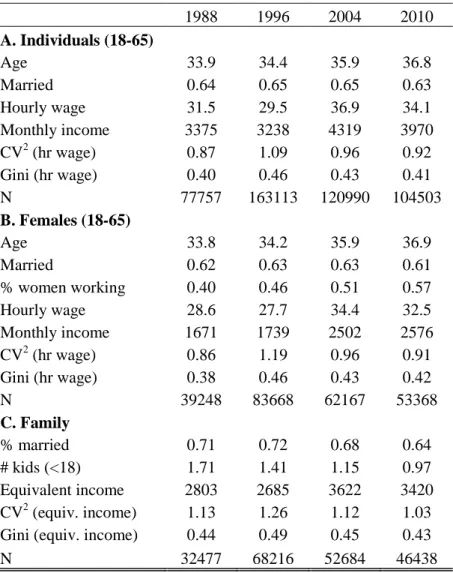
[Table 1 here]
Table 1 includes the number of observations at the individual and family level and descriptive statistics for year 1988, 1996, 2004 and 2010. Panel A shows information at the individual level for the age group 18-65, Panel B corresponds to females and Panel C to families. Mean age has continuously increased over time from 33 to 36 years, the proportion of married individuals was constant before 2004 and there is a slight decline in marriage rates from 2004 to 2010.18 The proportion of women working increased from 0.4 in 1988 to 0.57 in 2010. As in previous findings (Esquivel, 2009; Lopez-Acevedo, 2006), we can see that inequality follows an inverted-U-shaped pattern. This pattern is similar both when we calculate inequality at the individual level, restricting to females or at the family level. Panel C shows that the proportion of married-couple families has not declined as much as the proportion of married individuals. The number of individuals less than 18 years old declined substantially in the last 20 years due to a decrease in fertility rates. Mean income (adjusted by
16
This government office is in charge of measuring and reporting official statistics about poverty rates in Mexico. http://www.coneval.gob.mx/
17
Inequality trends are similar across different equivalence scales (per capita, square root of household size).
18
16
equivalence scales) decreased for the period 1988-1996 (due to the 1995 macroeconomic crisis) and then it increased.
[Figure 1 here]
Figure 1 depicts the percent of families in each of the four types previously described. The proportion of married-couple families decreased 7 percentage points in the last 20 years. The percent of households in which one spouse is not present, which represents only a small fraction (less than 2 percent) of the total, barely changed. On the other hand, the number of families conformed by one individual, headed by divorced, separated, or widowed
individuals increased (driven mainly by single families).
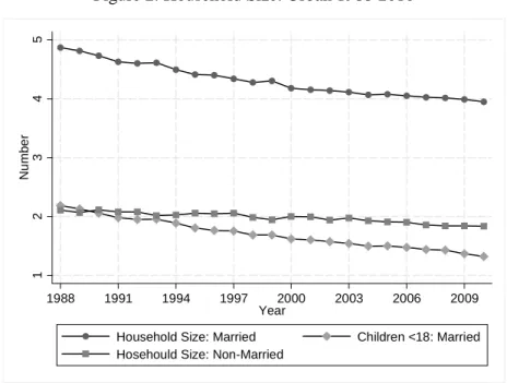
Figure 2 shows the family size for different types of families. For married-couple families, it decreased approximately by one member in the last 20 years. This is mainly driven by decreases in fertility as we can observe for the number of members less than 18 years old. On the other hand, family size for all other families has kept fairly constant at around 2 members per family.
[Figure 2 here] [Figure 3 here]
17
points. Panel B shows the patterns of female labor supply for married females with children (less than 6 years old) and other married females, as well as for non-married females with no children. The increase in female labor supply is more pronounced among married females with no children. When we calculate labor supply by education group (panel C), we find a rapid increase in female labor supply for individuals with low education.19 Females in the two lowest categories increased their labor supply more rapidly than females with high school or college degrees.
[Figure 4 here]
Figure 4 shows the proportion of women working and mean married females' income ranked by household's income. The x-axis in both panels corresponds to the quintile of family equivalent income distribution once we take out married females' income. Panel A suggests that families with low family income have a higher proportion of married females working. However, as family income increases (quintile 2 and above), the percent of working married females remains almost the same. There are some important differences across time. From 1988 to 1996, there is a higher increase in the percent of working married females in high income households than married females in middle income households. After 1996, married females in quintiles 1 to 4 increased their labor force participation more than those in quintile 5.
Panel B shows the mean wife income for each quintile of the family income
distribution. It shows that mean income in quintile 1 is higher than in quintile 2 due to the
19
18
high attachment of married females to the labor market. Married females in rich families earn relatively more than in families in quintile 2 to 4. In general, figure 4 shows that women married to men in quintile 5 have not increased their labor supply as other married females after 1996. Moreover, from 1988 to 1996 there was a marked increased in earnings for married females in high income households. Also, in the period 1996-2010 there was a higher relative increase in income for married females in quintiles 1-4 than that for married females in quintile 5.
In sum, previous results show that female labor supply increased in the last 20 years. This rise is particularly relevant for married females and for females with low education. Additionally, married females in high income families increased their labor force
participation and earnings relatively more during the period 1988-1996 than in 1996-2010. The next sections show the formal calculations investigating the effect of married females income on family income inequality.
5. Results
19
substantially lower than in countries such as Denmark and Sweden.20
Panel B in figure 5 shows that the correlation among income sources has barely changed in the last 20 years. Although the correlations fluctuate every year, the long-run relationships are stable. The correlation between married males' and married females' income is positive and, on average across time, equal to 0.28 (in 1988 it is equal to 0.27 and in 2010 to 0.28). This number is high in comparison to the results of studies for other countries. For the U.S., Cancian and Reed (1999) find that the correlation between married males' and married females' income is close to 0.22 in 1994, and they also show an increase in the correlation equal to 0.10 from 1967 to 1994. Moreover, Del Boca and Pasqua (2003) find that the correlation in Italy in 1998 is 0.21, although they show a correlation of 0.26 for North Italy. Also, Pasqua (2008) shows that the correlation between married males' and married females' income across OECD countries is fairly low and close to zero, only Portugal has a correlation close to 0.30. Amin and Da Vanzo (2004) find a correlation value equal to 0.13 in 1988 in Malaysia. Hence, a correlation of 0.28 is larger than those in the U.S., Italy, Malaysia and most OECD countries. As far as we are concerned, this result for Mexico was not previously known. On the other hand, both the correlation of married males' and other sources' income and the correlation of married females' and others sources' income are close to -0.08.
[Figure 5 here] [Figure 6 here] [Figure 7 here]
20
20
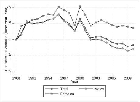
Figure 6 shows the trends of inequality at the invidual and household level. In order to analyze income inequality trends, we normalize the coefficient of variation by its 1988 level. Panel A shows an increase in inequality for all individuals, males and females for the period 1988-1996. After 1996, we observe a decline in inequality with the exception of years 2000-2001. In Panel B, inequality at the individual or household level follows a similar pattern. Since male inequality turns out to be the main determinant for individual income inequality, male inequality is more similar to household inequality than female inequality. In fact, Panel A shows that female income inequality has not decreased as much as male inequality since 2002. In sum, inequality follows an inverted-U shape pattern either at the individual or household level.
Although the patterns of individual income inequality are important to show similarity between individual and household inequality, the main goal of the paper is to analyze the contribution of married females’ earnings to total household inequality. Following the decomposition in equations (1) and (2), Figure 7 shows the evolution of family income inequality using the coefficient of variation for each source of income among married-couple families and for all families. Panel A shows inequality for married males, married females, other sources and families formed of unmarried individuals. Inequality decreased the most for married males and married females. Inequality for other sources barely changed and inequality for unmarried individuals slightly decreased for the period 1996-2010.21 Panel B shows the pattern of inequality for both married-couple and non-married-couple families. Inequality for married-couple families decreases substantially after 1996. In general, figures 6 and 7 show an inverted-U-shaped pattern in family income inequality during the period
21
21
1988-2010. This pattern is robust to changes in the inequality index.22
[Figure 8 here]
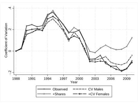
Now we present the results of the counterfactual computations described in Section 3. Each counterfactual facilitates our understanding of the role of married females' earnings in inequality. First, we calculate the contribution of married males income inequality using equation (1). In particular, we fix all parameters to their 1988 level and only let male inequality to change. Then, we analyze the contribution of married females, i.e. share of income and inequality of married females. If we first vary the share of income before female inequality, we are simulating the effect of a higher income to women that were participating in the labor market in 1988. Nevertheless, female labor supply increased, especially for women in poor families. Hence, we expect an increase in inequality with this counterfactual as women from poor families increased their labor supply and equation (1) assumes the “same women” as in 1988 are increasing their share of income. As it is difficult to separate the net effect of female labor supply from both 𝑆𝑤2 and 𝐶𝑉𝑤2, we argue that the combined effect is the contribution of married females to family income inequality. The difference between the last counterfactual (combined effect of married males and females) and observed inequality is the contribution of the rest of the parameters, i.e. correlations of earnings among members of the family and inequality of residual income. Finally, we can use equation (2) to calculate the effect of marriage rates on total income inequality. In particular, we calculate inequality among married households from the previous
22
22
counterfactuals, fix the marriage rate to its 1988 level and let inequality vary among non-married households.
Figure 8 shows the main results. In Panel A we plot observed inequality and inequality for each counterfactual with the following ordering using equation (1): 1. 𝐶𝑉𝑚2, 2.
𝑆𝑤2, 3.𝐶𝑉𝑤2. Panel B plots inequality among all households using equation (2) fixing the
marriage rate to its 1988 value but letting inequality of non-married households change as it did. In Panel A, we observe that even when fixing all parameters to their 1988 value, the main determinant of family inequality is married male inequality. 23 This is consistent with a larger share of husbands’ income. As males are the breadwinners of the households in our sample, inequality of married males is the main determinant of family income inequality.
Next we show the effect of varying both 𝐶𝑉𝑚2 and 𝑆𝑤2 (line that says “+Shares”). We observe an increase in family inequality especially in the 2000-2010 decade. This is
consistent with the recent increase in female labor supply among poor families. Allowing an increase in the share of income of married females is equivalent to saying that the “same women” that were participating in 1988 are participating in each year but with a larger share of income. When 𝐶𝑉𝑚2, 𝑆𝑤2 and 𝐶𝑉𝑤2 in equation (1) change as they did and the rest of the parameters are fixed to their 1988 level, we calculate the net effect of the increase in female labor supply and the change in the wage structure. Indeed, Panel A shows that inequality decreases and it is very similar to observed inequality which means that the rest of the parameters are relatively unimportant to explain changes in inequality.
Panel A summarizes the main results in the paper. First, married male income inequality is the main determinant of family income inequality. Second, both the female
23
23
labor supply and wage structure of married females contributed to a decrease in family income inequality. Finally, the correlation of earnings within the family has virtually no effect on inequality. Using all households and the previous counterfactuals, Panel B shows the effect of marriage rates on total inequality. We observe that had marriage rates kept constant at their 1988 level, total inequality would have been lower.
[Figure 9 here]
One critique to the decomposition exercise is that order matters. It is possible that the magnitudes of the contribution of each component change if we reverse the ordering. Hence, in order to analyze this possible effect among married households, we calculate the average contribution of married males, females (both share of income and inequality) and other components. Figure 9 shows the results.
The figure shows that the contributions of each component in Figure 8 are robust to the ordering. Male inequality is the main determinant of family income inequality. Married females contribute to equalize the family income distribution in the decade 2000-2010. If female labor supply had not changed, family income inequality would have been higher. Finally, the contribution of the correlation of earnings and residual income to family inequality is practically zero.
6. How do females affect the income distribution?
24
increased relatively more for low-skilled groups. In this section, we briefly analyze how married females affect the income distribution.
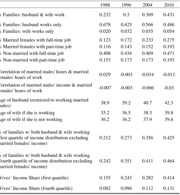
[Table 2 here]
Table 2 shows how different characteristics have evolved over time. As previously shown, married females have increased their labor supply over time. However, this could be due to an increase in non-working married males. The first three rows in the table present the percent of families according to husband and wife working status. Indeed, the percent of families in which both husband and wife work has been growing in the last 20 years. The percent of families in which both husband and wife worked in 1988 was 23 percent, but by 2010 this figure increased up to 43 percent. The next three rows show that the increase in female labor supply is mainly through full-time jobs, especially for married females.
Is this increase in female labor supply related to changes in married males' income or married males' working hours? Results presented in Table 2 show that this is not the case. Both correlations (rows 8 and 9) are close to zero. Hence, the increase in female labor supply does not seem to be related to changes in married males' employment conditions. It is also possible that the increase in married females' labor supply is due to new cohorts. If this is the case, we should observe a decrease or a differentiated pattern in age between married females that work and do not work. However, Table 2 shows that changes in average age over time for married females that work and do not work are very similar. This suggests that the increase in female labor supply is not restricted to younger cohorts.
25
income). This percentage increased more for richer families during the period 1988-1996. However, the gap diminished in the period 1996-2010. The percent of families in which both husband and wife work in the first quartile increased 15 percentage points during 1996-2010, while for the fourth quartile it only increased 11 points. Moreover, the last two rows in the table show a marked increase in the share of income for married females in poor families (first quartile), it goes from 13 percent in 1988 to 41 percent in 2010.24 Based on these findings and also those in figures 3 and 4, we consider that the increase in married females' labor supply, especially from low income families, contributed to the decrease in family income inequality.25
7. Conclusions
Income inequality in Mexico has followed an inverted-U-shaped pattern in the last 25 years. At the same time, female labor force participation increased substantially, especially for low skilled female workers. For this period we analyze whether changes in married females' earnings in married-couple families and marriage rate changes had an equalizing effect on the family income distribution. Using data from urban zones in Mexico for the period 1988-2010, we compare observed family income inequality (using equivalence scales) with counterfactual distributions under a number of different assumptions.
Among maried households, we find that married male income inequality is the main determinant for family income inequality. Second, both the female labor supply and wage
24
The increase in the share of income may be due to a higher proportion of non-working husbands. When dropping all families with zero income excluding married females' income, we get similar results. In this case, wives' income share in 1988 is 8.8 percent and 8.2 percent in the first and fourth quartile respectively, while in 2010 we get 16.1 percent and 12.9 percent in the first and fourth quartile respectively. Hence, even when we drop families with zero income (excluding wives' income) we observe a higher increase in income among poorer families.
25
26
structure of married females contributed to a decrease in family income inequality. Finally, the correlation of earnings within the family does not affect income inequality. On the other hand, for all households, had marriage rates kept constant at the 1988 level, inequality would have been lower.
Although female labor supply augmented for all groups, the rise was higher for married females, low-skilled females, and married females in poor families. We also find that the correlation between married males' and married females' earnings has been fairly stable at around 0.28 which is one of the highest values recorded in similar studies. Hence, we consider that family income inequality did not fall because of a reduction in income assortative mating, its decrease is driven by the increment in married females' labor supply for poor households and also by a reduction of inequality among female partners.
One final caution has to be noted. We only consider the effect of market female labor supply but we neglect the importance of housework. Our data does not allow us to check whether total hours of work for married females (market plus housework) has changed over time. Hence, we are unable to point out possible welfare effects at the family level. Although the welfare effects on families are beyond the scope of our paper, it might be the case that the increasing participation of married females in the labor market occurs at the expense of their leisure time if married females remain in charge of housework and childcare. Moreover, we do not address behavioral components of the effect of married males’ labor supply on married females’ earnings or the effect of household structure on inequality or labor participation. Future research is needed in order to address these issues.
27
Amin, S., and DaVanzo, J. (2004). “The Impact of Wives’ Earnings on Earnings Inequality among married-couple households in Malaysia.” Journal of Asian Economics, 15(1), pp. 49- 70. Aslaksen, I., Wennemo, T., and Aaberge, R. (2005). “Birds of a Feather Flock Together: The Impact
of Choice of Spouse on Family Labor Income Inequality.” Labour, 19(3), pp. 491-515. Bosch, M., and Manacorda, M. (2008). “Minimum Wages and Earnings Inequality in Urban Mexico:
Revisiting the Evidence.” CEP Discussion Paper 880, Centre for Economic Performance, London.
Campos-Vazquez, R. M. (2010). “Why did Wage Inequality decrease in Mexico after NAFTA?” Serie Documentos de Trabajo 15, El Colegio de México, Centro de Estudios Económicos, Mexico City.
Cancian, M., and Reed, D. (1998). “Assessing the Effects of Wives’ Earnings on Family Income Inequality.” The Review of Economics and Statistics, 80(1), pp. 73-79.
Cancian, M., and Reed, D. (1999). “The Impact of Wives’ Earnings on Income Inequality: Issues and Estimates.” Demography, 36(2), pp. 173-184.
Cragg, M., and Epelbaum, M. (1996). “Why has Wage Dispersion Grown in Mexico? Is it the Incidence of Reforms or the Growing Demand for Skills?” Journal of Development Economics, 51(1), pp. 99-116.
Daly, M. C., and Valleta, R. G. (2006). “Inequality and Poverty in the United States: The Effects of Rising Dispersion of Men’s Earnings and Changing Family Behavior.” Economica, 73(289), pp. 75-98.
Davies, H., and Joshi, H. (1998). “Gender and Income Inequality in the UK 1968-1990: the Feminization of Earnings or of Poverty?” Journal of the Royal Statistical Society. Series A (Statistics in Society), 161(1), pp. 33-61.
Del Boca, D., and Pasqua, S. (2003). “Employment Patterns of Husbands and Wives and Family Income Distribution in Italy (1977-98).” Review of Income and Wealth, 49(2), pp. 221-245. DiNardo, J., Fortin, N. M., and Lemieux, T. (1996). “Labor Market Institutions and the Distribution
of Wages, 1973-1992: A Semiparametric Approach.” Econometrica, 64(5), pp. 1001-1044. Esquivel, G. (2009). “The Dynamics of Income Inequality in Mexico since NAFTA.” Regional
Bureau for Latin America and the Caribbean Research for Public Policy Inclusive
Development Working Paper ID-02-2009, United Nations Development Programme, New York.
28
Latin America. A Decade of Progress? (Washington, DC.: Brookings Institution ), chap. 7, pp. 175 -217.
Esquivel, G., and Rodríguez-López, J. A. (2003). “Technology, Trade and Wage Inequality.” Journal of Development Economics, 72(2), pp. 543-565.
Fairris, D. (2003). “Unions and Wage Inequality in Mexico.” Industrial and Labor Relations Review, 56(3), pp. 481-497.
Ferreira, F., De Ferranti, D., Perry, G. E., and Walton, M. (2004). Inequality in Latin America: Breaking with History? (Washington, DC.: World Bank).
García, B. (2001). “Reestructuración Económica y Feminización del Mercado de trabajo en México.”
Papeles de Población, 27, pp. 45-61.
Gottschalk, P., and Danziger, S. (2005). “Inequality of Wage Rates, Earnings and Family Income in the United States, 1975-2002.” Review of Income and Wealth, 51(2), pp. 231-254.
Harkness, S. (2010). “The Contribution of Women’s Employment and Earnings to Household Income Inequality: A Cross Country Analysis.” Luxembourg Income Survey, Working Paper Series 531, Luxembourg.
Johnson, D., and Wilkins, R. (2004). “Effects of Changes in Family Composition and Employment Patterns on the Distribution of Income in Australia: 1981-1982 to 1997- 1998.” Economic Record, 80(249), pp. 219-238.
Juhn, C., and Murphy, K. M. (1997). “Wage Inequality and Family Labor Supply.” Journal of Labor Economics, 15(1), pp. 72-97.
Katz, L., and Autor, D. (1999). “Changes in the Wage Structure and Earnings Inequality,” in O. Ashenfelter, and D. Card (eds) Handbook of Labor Economics (Amsterdam: North Holland), vol. 3C, pp. 1463-1555.
Lehrer, E. L. (2000). “The Impact of Women’s Employment on the Distribution of Earnings among married-couple households: a comparison between 1973 and 1992-1994.” The Quarterly Review of Economics and Finance, 40(3), pp. 295-301.
Lopez, J. H., and Perry, G. (2008). “Inequality in Latin America: Determinants and Consequences.” Policy Research Working Paper 4504, The World Bank, Washington, DC.
Lopez-Calva, L. F., and Lustig, N. (2009). “The Recent Decline of Inequality in Latin America: Argentina, Brazil, Mexico and Peru.” Working Papers 140, ECINEQ, Society for the Study of Economic Inequality, Palma de Mallorca.
29
Lustig (eds) Declining Inequality in Latin America. A Decade of Progress? (Washington, DC.: Brookings Institution ), chap. 1, pp. 1-24.
López-Acevedo, G. (2006). “Mexico: Two Decades of the Evolution of Education and Inequality.” World Bank Policy Research Working Paper 3919, The World Bank, Washington, DC. Machado, J. A. F., and Mata, J. (2005). “Counterfactual Decomposition of Changes in Wage
Distributions using Quantile Regression.” Journal of Applied Econometrics, 20(4), pp. 445-465.
Machin, S. (2008). “An Appraisal of Economic Research on Changes in Wage Inequality.” Labour, 22(Special Issue), pp. 7-26.
Martin, M. A. (2006). “Family Structure and Income Inequality in Families with Children, 1976 to 2000.” Demography, 43(3), pp. 421-445.
McKenzie, D. J. (2003). “How do Households Cope with Aggregate Shocks? Evidence from the Mexican Peso Crisis.” World Development, 31(7), pp. 1179-199.
Parker, S. and E. Skoufias (2004). “The Added Worker Effect over the Business Cycle: Evidence from Urban Mexico.” Applied Economic Letters, 11(10), pp. 625-630.
Parker, S. and E. Skoufias (2006). “Job Loss and Family Adjustment in Work and Schooling during the Mexican peso crisis.” Journal of Population Economics, 19(1), pp. 163-181.
Pasqua, S. (2008). “Wives’ Work and Income distribution in European Countries.” European Journal of Comparative Economics, 5(2), pp. 157-186.
Rendón, T. (2003). “Empleo, Segregación y Salarios por Género,” in E. de la Garza Toledo, and C. S. Páez (eds) La Situación del Trabajo en México, (México City: Plaza y Valdés), chap. VI, pp. 129-150.
Robertson, R. (2007). “Trade and Wages: Two Puzzles from Mexico.” The World Economy, 9(30), pp. 1378-1398.
Sotomayor, O. J. (2009). “Changes in the Distribution of Household Income in Brazil: The Role of Male and Female Earnings.” World Development, 37(10), pp. 1706-1715.
30
Table 1. Descriptive Statistics
1988 1996 2004 2010
A. Individuals (18-65)
Age 33.9 34.4 35.9 36.8
Married 0.64 0.65 0.65 0.63
Hourly wage 31.5 29.5 36.9 34.1
Monthly income 3375 3238 4319 3970
CV2 (hr wage) 0.87 1.09 0.96 0.92
Gini (hr wage) 0.40 0.46 0.43 0.41
N 77757 163113 120990 104503
B. Females (18-65)
Age 33.8 34.2 35.9 36.9
Married 0.62 0.63 0.63 0.61
% women working 0.40 0.46 0.51 0.57
Hourly wage 28.6 27.7 34.4 32.5
Monthly income 1671 1739 2502 2576
CV2 (hr wage) 0.86 1.19 0.96 0.91
Gini (hr wage) 0.38 0.46 0.43 0.42
N 39248 83668 62167 53368
C. Family
% married 0.71 0.72 0.68 0.64
# kids (<18) 1.71 1.41 1.15 0.97
Equivalent income 2803 2685 3622 3420
CV2 (equiv. income) 1.13 1.26 1.12 1.03
Gini (equiv. income) 0.44 0.49 0.45 0.43
N 32477 68216 52684 46438
Source: Authors’ calculations with data from INEGI.
31
Table 2. Female Statistics
1988 1996 2004 2010
% Families: husband & wife work 0.232 0.3 0.369 0.431
% Families: husband works only 0.678 0.625 0.566 0.486
% Families: wife works only 0.020 0.032 0.035 0.054
% Married females with full-time job 0.123 0.172 0.233 0.275
% Married females with part-time job 0.116 0.143 0.152 0.193
% Non-married with full-time job 0.408 0.434 0.469 0.471
% Non-married with part-time job 0.153 0.173 0.173 0.193
Correlation of married males' hours & married
females' hours of work 0.029 -0.003 -0.014 -0.011
Correlation of married males' income & married
females' hours of work -0.007 -0.003 -0.006 -0.03
Age of husband (restricted to working married
males) 38.9 39.2 40.7 42.3
Age of wife if she is working 35.2 36.5 38.3 39.8
Age of wife if she is not working 36.2 36.2 37.9 39.6
% of families w/ both husband & wife working (first quartile of income distribution excluding married females' income)
0.212 0.273 0.356 0.425
% of families w/ both husband & wife working (fourth quartile of income distribution excluding married females' income)
0.242 0.351 0.411 0.464
Wives’ Income Share (first quartile) 0.155 0.243 0.282 0.414
Wives’ Income Share (fourth quartile) 0.082 0.096 0.112 0.131
Source: Authors’ calculations with data from INEGI.
32
Figure 1: Type of Households. Urban 1988-2010
Source: Authors’ calculations with data from INEGI.
Notes: Sample restricted to urban households. Final sample excludes households with zero income and households in which the age of the household head is outside the range 18-65. "Married: Husband & Wife" refers to both spouses living together in the household. "Married: no spouse" refers to families in which the household head declares to be married but the spouse does not live in the household. "Single, Divorced, etc" refers to families declaring as civil status to be separated, divorced, or widowed with no cohabitation. "Singles living alone" refers to singles either because they live alone, or have no relationship with the household head.
0
.2
.4
.6
.8
Sh
a
re
1988 1991 1994 1997 2000 2003 2006 2009
Year
33
Figure 2: Household Size: Urban 1988-2010
Source: Authors’ calculations with data from INEGI.
Notes: Sample restricted to urban households. Final sample excludes households with zero income and households in which the age of the household head is outside the range 18-65. Figure shows household size for urban households. "Children<18: Married" refers to the number of individuals less than 18 years old living in married households.
1
2
3
4
5
Nu
m
be
r
1988 1991 1994 1997 2000 2003 2006 2009
Year
34
Figure 3: Female Labor Supply. Urban 1988-2010
Panel A. Total Panel B. Type of Household
Panel C. Education Groups
Source: Authors’ calculations with data from INEGI.
Notes: Sample restricted to urban households. Labor supply defined as individuals with positive hours of work. Panel A refers to female labor supply of married and non married groups. Panel B is the same as panel A but divides married females into females with children less than 6 years old and the rest. Panel C refers to female labor supply for both married and non-married by education groups.
.15 .25 .35 .45 .55 .65 .75 Sh a re
1988 1991 1994 1997 2000 2003 2006 2009 Year
Married: Spouse present Other
.15 .25 .35 .45 .55 .65 .75 Sh a re
1988 1991 1994 1997 2000 2003 2006 2009 Year
Married & Child<6 Other Married Non-Married and no children
.15 .25 .35 .45 .55 .65 .75 Sh a re
1988 1991 1994 1997 2000 2003 2006 2009 Year
35
Figure 4: Female Labor Supply and Female Income by Household Income. Married & Urban Households 1988-2010
Panel A. Female Labor Supply by Household’s Income
Panel B. Female Income by Household’s Income
Source: Authors’ calculations with data from INEGI.
Notes: Sample restricted to urban households. Final sample excludes households with zero income and households in which the age of the household head is outside the range 18-65. Furthermore, sample is restricted to married households (both husband and wife living together) with positive income. Panel A refers to female labor supply according to the quintile of the income distribution for the rest of the household (total family income less wife’s income). Income is adjusted using equivalence scales as described in the text. Panel B refers to mean female income according to the quintile income distribution for the rest of household’s income. Income is in real terms (January 2010 pesos).
.2 .3 .4 .5 .6 .7 % W or k ing
1 2 3 4 5
Quintile 1988 1996 2004 2010 20 0 40 0 60 0 80 0 10 00 12 00 M ea n I nc o m e F em a le
1 2 3 4 5
Quintile
1988 1996
36
Figure 5: Share of Income and Correlations among Married Families. Urban 1988-2010 Panel A. Share of Income
Panel B. Correlations
Source: Authors’ calculations with data from INEGI.
Notes: Sample restricted to urban households. Final sample excludes households with zero income and households in which the household head age is outside the range 18-65. Furthermore, sample is restricted to married households. Panel A measures the share of income of each source and panel B the correlation among income sources. 0 .1 .2 .3 .4 .5 .6 .7 .8 .9 Sh a re o f I n co me
1988 1991 1994 1997 2000 2003 2006 2009
Year Husbands Wives Others -. 1 -. 05 0 .05 .1 .15 .2 .25 .3 .35 Co rr el at io n Co ef fic ie nt
1988 1991 1994 1997 2000 2003 2006 2009
Year
37
Figure 6: Coefficient of Variation. Urban 1988-2010 Panel A. Individuals
Panel B. Individual vs Household Inequality
Source: Authors’ calculations with data from INEGI.
Notes: Sample restricted to urban households. Base year is 1988. Individual inequality sample restricts to individuals between 18 and 65 years old. Household inequality sample excludes households with zero income and households in which the age of the household head is outside the range 18-65. We use total labor income for the inequality calculations. Hourly wage inequality follows a similar trend.
-. 3 -. 15 0 .15 .3 C oe ff ic ien t of V a ria ti on ( B a s e Y ea r 1 98 8)
1988 1991 1994 1997 2000 2003 2006 2009
Year Total Males Females -. 3 -. 15 0 .15 .3 C oe ff ic ien t of V a ria ti on ( B a s e Y ea r 1 98 8)
1988 1991 1994 1997 2000 2003 2006 2009
Year
38
Figure 7: Coefficient of Variation by Type of Family. Urban 1988-2010 Panel A. Married Households
Panel B. All Households
Source: Authors’ calculations with data from INEGI.
Notes: Sample restricted to urban households. Final sample excludes households with zero income and households in which the age of the household head is outside the range 18-65. Panel A calculates the coefficient of variation of each income source for married households. Panel B calculates the coefficient of variation by type of household.
.8 1. 4 2 2. 6 3. 2 Co ef fic ie nt of V ar ia tion
1988 1991 1994 1997 2000 2003 2006 2009
Year Husbands Wives Others Non-Married .6 .8 1 1 .2 1 .4 C oe ff ic ien t of V a ria ti on
1988 1991 1994 1997 2000 2003 2006 2009
Year
Total Married
39
Figure 8: Counterfactual distributions. Urban 1988-2010
Panel A. Married Households-One component at a time
Panel B. All Households-Marriage Rates constant
Source: Authors’ calculations with data from INEGI.
Notes: Sample restricted to urban households. Final sample excludes households with zero income and households in which the age of the household head is outside the range 18-65. Results are presented using year 1988 as the base year (both observed and counterfactual inequality start in zero in 1988).
-.2
0
.2
.4
C
oef
fi
c
ient
of
V
ar
iat
ion
1988 1991 1994 1997 2000 2003 2006 2009
Year
Observed CV Males
+Shares +CV Females
-.2
0
.2
.4
C
oef
fi
c
ient
of
V
ar
iat
ion
1988 1991 1994 1997 2000 2003 2006 2009
Year
Observed CV Males
40
Figure 9: Robustness test. Average contribution of all counterfactuals. Married Households.
Source: Authors’ calculations with data from INEGI.
Notes: Sample restricted to urban households. Final sample excludes households with zero income and households in which the age of the household head is outside the range 18-65. Results are presented using year 1988 as the base year (both observed and counterfactual inequality start in zero in 1988).
-.2
0
.2
.4
C
ont
ri
but
ion
to C
V
1988 1991 1994 1997 2000 2003 2006 2009
Year
Observed Males