An analysis of the relationship between wages in the public and private sector in colombia : a panel data approach

SERIE DO C UM ENTO S DE TRA BA JO

No . 9 7

A b ril 2 0 1 1

AN ANALYSIS OF THE RELATIONSHIP BETWEEN WAGES IN

THE PUBLIC AND PRIVATE SECTOR IN COLOMBIA:

A PANEL DATA APPROACH

Jesús Otero

An analysis of the relationship between wages in

the public and private sector in Colombia:

A panel data approach

Jesús Otero

Facultad de Economía

Universidad del Rosario

Bogotá, Colombia

Luis Fernando Gamboa

Facultad de Economía

Universidad del Rosario

Bogotá, Colombia

Andrés García-Suaza

Facultad de Economía

Universidad del Rosario

Bogotá, Colombia

April 2011

Abstract

This document examines the time-series properties of the wage di¤erentials that arise between the public and private sector in Colombia during the sample period 1984 to 2005. We …nd con‡icting results in unit-root and stationarity tests when looking at wage di¤erentials at an aggregate level (such as for men, women or both). However, when we analyse wage di¤erentials at higher levels of disaggregation, treat them jointly as a panel of data, and allow for the presence of potential cross section dependence, there is more supportive evidence for the view that wage di¤erentials are stationary. This implies that although wage di¤erentials do exist, they have not been consistently increasing (or decreasing) over time.

The authors gratefully acknowledge the …nancial support from Centro de Gestión del Conocimiento y la Innovación – Universidad del Rosario (Project FIUR – DVG 080). We would also like to thank Monica Giulietti for useful discussions on several of the ideas developed in the paper. Oscar Avila provided excellent research assistance. Any remaining errors are ours.

1

Introduction

Historically, the role and the size of the public sector have been topics of consider-able debate among economists. In this debate, both employment and remuneration in public sector labour markets have usually been at the core of the discussion. Clearly, these two issues are of importance because of their economic and social policy dimensions, as wages constitute the main source of income for a large number of individuals and their families. In addition, wages serve as the mechanism that guides not only an individual’s work-leisure decision problem, but also his/her choice of where to work.

It is well known that economic theory establishes that wages are positively re-lated to labour productivity. However, when it comes to the public sector the question of how wages and employment are determined is not easy to answer. As indicated by Gregory and Borland (1999), while in the private sector employment and earnings are determined within a market environment, in the public sector the same decision-making process takes place within a political environment, where politicians and bureaucrats may well have objective functions that di¤er from those utilise by the owners of …rms in the private sector. Thus, for example, a politi-cian’s objective function may well be one of vote-maximisation, or alternatively one of budget-maximisation. In addition to this, the e¤ects of unions and collective bargaining are more likely to be observed in public sector labour markets than in private ones.

The purpose of this document is to study the relationship between wages in the public and private sector in Colombia. During the last two decades or so, Colombia has become an interesting case-study that features high and persistent unemployment, low rates of job creation in the formal private sector, and the growing importance of an informal private sector that is characterised by new contractual forms in the labour market.1 _{These new contractual forms include the creation of}

1_{Lora and Márquez (1998) present some stylised facts of employment in Colombia as well as in}

companies whose main objective is to act as intermediaries between workers and …rms, where the latter aim to minimise the payroll taxes associated to the formal sector, which include social security payments and pension contributions, among others. As a result, jobs in the public sector become more attractive due to the fact that it is more di¢cult for employers to avoid the payment of these additional costs to their employees.

International literature on the evolution of wages in the public and private sectors and the corresponding di¤erential that arises between them is extensive; see, inter alia, Pederson, Schmidt-Sørensen, Smith, and Westergård-Nielsen (1990), Hundley (1991), Mueller (1998), Tansel (1998), Adamchik and Bedi (2000), Bender (2002), Panizza and Qiang (2005) and Lamo, Perez, and Schuknecht (2008). Literature for Colombia is more scarce. Two relatively recent exceptions are Arango and Posada (2007), who present a descriptive analysis of the dynamic behaviour of public sec-tor wages in several occupational categories, and Galvis (2010), who studies wage disparities for private sector employees. Based on our literature review, it appears that there are no other works for Colombia that analyse the behaviour of public and private sector wages, both within each sector as well as between them.

The main objective of this document is to examine whether there is evidence of a stable long-run equilibrium relationship between wages in the public and pri-vate sector in Colombia. We believe that the study of the Colombian experience is interesting because ever since 1886, the central government concentrated political, administrative and …scal powers. Then, in 1991 a constitutional reform introduced important modi…cations and changes in the existing territorial order of the country, so that regional and local levels of government were given greater power and respon-sibilities, and a new set of parameters to assign and determine transfers from the central government were de…ned.2 _{Thus, it is of some interest to determine whether}

this decentralisation process has led to increasing wage di¤erentials between sec-tors. Initially, this analysis can be undertaken at an aggregate level by comparing

earnings in the private sector with those in the public sector. Then, one could fur-ther analyse gender, city and occupational category di¤erentials between public and private sector employees.

This document o¤ers three main contributions to existing literature. First, we use data from Colombian household surveys collected over the period 1984 to 2005. The advantage of this source of information is that it allows us to focus on how individual-level data have changed over time for di¤erent economic sectors, gender, occupational category and city. The selection of the sample period is dictated by the availability of a consistent dataset. This is because in 2006 signi…cant methodological changes were implemented in the household survey system, so that results before and after this year are not directly comparable.

Second, we focus on an examination of the time series properties of wage di¤eren-tials or, put another way, we assess whether or not wage di¤erendi¤eren-tials are stationary. In this sense, …nding that a wage di¤erential is stationary is equivalent to saying that the two wages are cointegrated with a known cointegrating vector equal to

[1; 1]0. From an economic point of view, this means that wage levels maintain a stable long-run equilibrium relationship, so that the corresponding wage di¤erential does not increase (or decrease) without bound as time passes. To the best of our knowledge, this empirical modelling approach has not been implemented by other authors.

Third, the time-series analysis will be undertaken by looking at each wage dif-ferential individually as well as within a panel data framework. The advantage of adopting a panel data setup is that it allows us to examine the potential e¤ect of cross-sectional dependence among wages that may arise from common shocks (or innovations). Another advantage of panel data is that by combining information from the time-series dimension with that from the cross-section dimension, fewer time series observations are required for statistical tests to have power.

methodology that will be used in the document. We start o¤ by brie‡y presenting important time-series concepts that will be used in the document, along with their economic implications. Then, we describe the statistical tests that will be applied to assess the time-series properties of several wage di¤erentials. Section 4 describes the data that will be used in the document and shows some of the stylised facts about the evolution of wages in Colombia. Section 5 examines the time-series properties of wage di¤erentials in the country. Section 6 o¤ers concluding remarks.

2

Brief literature review

During the last three decades or so, a number of authors have analysed the dynamic behaviour of public and private sector wages. The study of wage di¤erentials between the public and private sectors has been motivated, among other factors, by the recent growth of the public sector in many countries around the world and the corresponding cost-implications on tax-payers. There are two main reasons why one should be interested in the operation of public sector labour markets. First, public sector labour markets are large and their …nancial resources primarily come from the functioning of the private sector. Second, public sector labour markets are di¤erent from private sector labour markets in as much as politicians or bureaucrats’ objective function di¤ers from that of the owners of private sector …rms. Indeed, as indicated in the previous section, decision-making on public sector employment and wages takes place in a political environment, where politicians and bureaucrats may have objectives that not always seek pro…tability. By contrast, private sector decision-making occurs in a market environment in which owners (or shareholders) of private sector …rms continuously monitor the performance of their companies.

literature that provides theoretical reasons that attempt to explain the existence of public/private wage di¤erentials. According to this author, there are several factors that may be taken into consideration when examining possible explanations. First, there is the in‡uence of trade unions on demand for public sector goods and the ‘vote producing’ activities by civil servants. Second, part of the public/private wage di¤erential may emerge from economic rents perceived by public sector workers be-cause of their bargaining power in those services that are considered essential. Third, the idea of a public/private wage di¤erential has to be analysed carefully because of the existence of selection bias and other econometric problems that may arise from the available data. According to Bender (2002) a common …nding of the empirical studies in his survey is the existence of a declining premium paid to central govern-ment employees, although for developing countries wage di¤erentials are found to be negative in some instances. As will be shown below, there are di¤erent ways to study the existence of wage di¤erentials between the public and private sectors. However, an important factor that must be taken into account, in particular for the purposes of international comparisons, is the size of the public sector in the economy, as it re‡ects the capacity of the sector to compete for workers in the labour market.

In their analysis of public sector labour markets, Gregory and Borland (1999) …nd a persistent increase in the size of the public sector in several countries. According to these authors, public sector workers get higher average earnings than private sector ones due to di¤erences in levels of education (which is higher for individuals in the public sector). At the same time, these authors also …nd that the earnings distribution of public sector workers exhibits is more concentrated around its mean value compared to that of private sector workers. In addition, the union/non-union and male/female wage gaps tend to be smaller in the public sector.

for Germany, Mueller (1998) for Canada, Tansel (1998) for Turkey, Adamchik and Bedi (2000) for Poland, and Lamo, Perez, and Schuknecht (2008) for a sample of OECD and Euro zone countries. Some of these studies have looked at the deter-minants of wages, while others have examined the existence of wage di¤erentials between the public and private sectors.

Pederson, Schmidt-Sørensen, Smith, and Westergård-Nielsen (1990) examine the public/private wage di¤erential using Danish data from a panel of individuals over the period 1976 to 1985. The results of estimating …xed-e¤ect type regressions show evidence that a wage-twist policy has been applied over the sample period. The idea of a wage-twist policy is to implement a series of mechanisms to a¤ect the allocation of resources between the public and the private sector. Thus, for example, a government may attempt to reduce the private/public wage di¤erential in order to overcome recruitment and retention problems for public sector employees. An additional interesting …nding form their work is that "women employed in the formal sector tend to have higher average skills than men employed in the formal sector (...) probably due to supply and demand considerations" (p. 830). According to these authors, if it is accepted that job security is important in the public sector, then the public wage premium has to be analysed from a di¤erent perspective, such as the general equilibrium one considered by Shapiro and Stiglitz (1984).

Hundley (1991), using data from the 1985 Current Population Survey of the United States, …nds that public/private wage di¤erentials tend to decline as the level of skill required to ful…l an occupational category is increased. Mueller (1998) uses quantile regression techniques to estimate the size of the public/private wage di¤erential in Canada. This author …nds that this di¤erential tends to be highest for women, federal government employees, and individuals at the lower tail of the wage distribution. The use of quantile regressions is crucial to understand di¤erences in public/private wages over the whole distribution of wages and not only at the mean of the distribution.

em-pirical models on public/private sector wage structures for Germany. They use an extended version of a standard switching regression model that allows for en-dogeneity in the level of education, experience, and hours worked. Several model speci…cations are estimated and the results of such models are subsequently com-pared. It turns out that their results are sensitive to the identi…cation assumptions that are adopted, but robust to the regressors that are included in the model. Al-varez, Jareño, and Sebastian (1993) use Spanish data over the period 1964–1991 to analyse transmission mechanisms between prices and nominal wages. The results of estimating a VAR model indicates that private sector wages help explain in‡ation, while public sector wages play a minor role. They also …nd that public sector wages do not have an impact on private sector wages.

Adamchik and Bedi (2000) examine whether there are wage di¤erentials between workers in the public and the private sectors in Poland. After standardising for worker characteristics and sector selection e¤ects, they …nd evidence of a private sector positive wage premium. This wage premium is particularly large for university educated workers. According to the authors, the existence of these wage di¤erentials make it di¢cult for the public sector to attract and retain skilled employees. In addition, lower public sector wages may encourage moonlighting and compromise the e¢ciency of the public sector.

di¤erentials because of gender are not found for individuals working in the public sector, although they are found to exist for workers in the private sector.

For Latin American countries, existing literature appears more scarce; see e.g. Panizza and Qiang (2005) for a study of a sample of Latin American countries, Stelcner, der Gaag, and Vijverberg (1989) for the case of Peru, and Arango and Posada (2007) and Galvis (2010) for studies of the Colombian case. Panizza and Qiang (2005) use household survey data for thirteen Latin American countries to investigate wage di¤erentials between the public and private sectors, as well as wage di¤erentials that may arise because of gender.3 _{These authors …nd that in the cases}

of Brazil, Colombia, Costa Rica, Ecuador and El Salvador, there is evidence of a statistically and economically signi…cant public wage premium that favours male workers. Interestingly, in the cases of Brazil, Colombia, Costa Rica, Honduras, Mexico and El Salvador, they also uncover evidence of a wage premium for women working in the public sector. Stelcner, der Gaag, and Vijverberg (1989) use Peruvian data to study the emergence of wage di¤erentials between male and female workers in the public and private sectors. The authors estimate a switching regression model and …nd that there is not a "pure" wage advantage or economic rent of government workers when corrected estimates of wage functions are compared. Their …ndings indicate that in Lima there is a wage di¤erential in favour of private sector employees, while in other urban areas there is no signi…cant wage di¤erential. In the case of Colombia, the evolution of the public and private sector wages has not received a great deal of attention. Two relatively recent exceptions are Arango and Posada (2007) and Galvis (2010). Arango and Posada (2007) present a descriptive analysis of the dynamic behaviour of public sector wages in several occupational categories. An interesting feature of this work is that the authors use payroll information from the Ministry of Finance, which covers the sample period 1978–2005. On the other hand, Galvis (2010) uses Colombian household survey data for the period 1984 to 2009, to study real wage disparities for private sector employees in the seven main

metropolitan areas, namely Barranquilla, Bogotá, Bucaramanga, Cali, Manizales, Medellín and Pasto. This author …nds that there are signi…cant di¤erentials among di¤erent categories of private sector wages, and that in some cases these di¤erentials have been growing over time.

3

Methodology

3.1

Background

Economists typically use information that is available in three di¤erent formats: (i.) cross-section data; (ii.) time-series data; and (iii.) panel data. Cross-section data describe the activities of individuals, …rms, countries or other units of analysis that are collected at a particular moment in time. Time-series data describe the movement of a variable through time, and this could be for di¤erent periodicity such as annual, quarterly, monthly, weekly or even daily. Lastly, panel data combine the …rst two types of information; that is, they describe the activities of individuals, …rms, countries or other units of analysis through time.

Focusing for the moment in the analysis of time-series data, the starting point is the concept of stationarity. A time-series is said to be stationary if its probability distribution function does not change through time. In practice, this de…nition turns out to be very strong and di¢cult to verify, so that a weaker version of the con-cept states that a time-series is "weakly stationary" (also referred to as "covariance stationary") if its …rst two moments (i.e. its mean and its variance) do not change over time. The intuition behind this de…nition is that if the …rst two moments of a time-series do not change through time, then its future is going to be similar to its past, and this can be exploited for forecasting purposes.

non-stationary series involves a number of problems in the sense that conventional hypothesis tests, con…dence intervals and predictions about the future are not go-ing to be reliable. A classic example of the problems that arise with the use of non-stationary data is that of the non-sense regression problem discovered by Yule (1926), or spurious regression problem in the terminology of Granger and Newbold (1974). The idea is that when one estimates a regression between two or more vari-ables that grow over time (whatever these varivari-ables may be), it is more likely than not that one is going to …nd an apparent positive association between the variables, regardless of whether this association truly exists.4

The solution to the problem of working with non-stationary series depends upon the nature or cause of the non-stationarity, that is whether it is deterministic or stochastic. Until the early 1980s, the trending behaviour of a time-series used to be eliminated by running a regression of the series under consideration against a linear (or even a polynomial) time trend. What this statistical approach does not recognise, however, is that it is only valid when the rate of growth of the series is always the same or, in other words, when it is constant. If, on the other hand, the rate of growth of the series is not always the same (or if it cannot be predicted perfectly), then the time series is said to have a stochastic trend, in which case the suitable approach to eliminate the non-stationarity would be to calculate the …rst di¤erence of the series.

In time-series terminology, a series that needs to be di¤erenced in order to become stationary is said to be a series integrated of order 1, and is denoted I(1) for short. In general, a series that needs to be di¤erenced d times in order to become stationary is said to be a series integrated of order d, and is denoted I(d). In summary, economic time-series that exhibit a trending behaviour can be classi…ed in two groups. The …rst group is that of the series that are stationary around a linear

4_{Examples of the spurious regression problem include Yule (1926) who, using annual information}

or polynomial trend, which are referred to as Trend Stationary Processes (TSP). The second group is that of the series that need to be di¤erenced one or many more times. Interestingly, it should be noticed that a stationary series is integrated of order 0, denoted I(0), since it is not necessary to di¤erence the series to make it stationary.

The fact that a time-series can be classi…ed as an I(0) or an I(1) process can have important implications from an economic point of view. Indeed, in the case of an I(0) series, a shock (or innovation) will have a temporary e¤ect (i.e. the e¤ect of the shock disappears as time passes) and out-of-sample predictions are more precise. On the contrary, in the case of an I(1) series, the e¤ect of a shock (or innovation) is permanent and out-of-sample predictions are less accurate; see e.g. Franses (1998). More importantly, while the variance an I(0) series is …nite, that of an I(1) series increases without a bound.

In the speci…c case of public/ private sector wage di¤erentials, which are the purpose of analysis of this document, …nding that they can be best characterised as

I(0) processes suggests that there would not be a tendency for them to consistently increase (or decrease) over time. On the contrary, if public/ private sector wage di¤erentials are found to be I(1), then there would be arbitrage opportunities for individuals by moving from one sector to the other. This, of course, may become a serious obstacle for governments that aim to attract and maintain a productive labour force in the public sector.

3.2

Unit-root and stationarity tests

During the late 1970s and early 1980s, Dickey and Fuller (1979) and Dickey and Fuller (1981) propose statistical tests to determine whether a time series can be best characterised as TSP or DSP. These statistical tests are referred to in the literature as unit-root tests.

yt= 1yt 1+ t; (1)

yt= 0 + 1yt 1+ _t; (2)

yt = 0+ 1yt 1+ 2t+ t; (3)

whereytis the variable of interest (in our case a wage di¤erential) for which we have

t = 1; :::; T available observations. These equations can be estimated by ordinary least squares (OLS), and the null hypothesis to test the presence of a unit root is

H0 : 1 = 1, against the alternative that the series is stationaryHa: 1 <1.

For practical purposes, model (1) is rarely estimated as it is too restrictive because it assumes that yt has a mean of zero (the model is very important for theoretical purposes though). In turn, model (2) is estimated when yt has a non-zero mean, while model (3) is applied wheneverytexhibits an upward (or downward) behaviour; for a more formal sequential testing procedure see Perron (1988). The models considered by Dickey and Fuller can be alternatively reparameterised as:

yt = ( 1 1)yt 1+ t;

yt= 0+ ( 1 1)yt 1+ t;

yt= 0+ ( 1 1)yt 1+ 2t+ t;

where yt is the …rst di¤erence of the series of interest, i.e. yt=yt yt 1. Notice

that testing the null hypothesis that H0 : 1 = 1 is equivalent to test H0 : b= 0 in

the following models:

yt = 0+byt 1+ t; (5)

yt= 0+byt 1+ 2t+ t: (6)

To perform the unit-root test, one calculates the t-statistic associated to the esti-mated coe¢cient on yt 1, which is then compared with the critical values tabulated

by Fuller (1976), Dickey and Fuller (1981), or the more recent response surfaces estimated by MacKinnon (1991).

An important assumption behind the construction of the Dickey and Fuller tests is that of no serial correlation, i.e. t iid(0;

2

). If this assumption does not hold, then Said and Dickey (1984) suggest introducing lags of the dependent variable in order to whiten the residuals. Including lags of the dependent variable in equations (4), (5) and (6) yields:

yt=byt 1+

p

X

i=1

i yt i+ t;

yt= 0 +byt 1+

p

X

i=1

i yt i+ t;

yt = 0+byt 1+ 2t+

p

X

i=1

i yt i+ t:

These three equations are referred to as the (Augmented) Dickey and Fuller (1979) (ADF) test regressions.

Kwiatkowski, Phillips, Schmidt, and Shin (1992) (KPSS) propose an alternative approach, in which the null and alternative hypotheses are interchanged. That is, they propose a residual-based Lagrange Multiplier (LM) tests for the null hypothesis that a time series is stationary (either around a level or a deterministic time trend), against the alternative that it is non-stationary.

yt= t+rt+ yt 1+"t;

where rt=rt 1+ut, "t is iid(0; 2

"),

2

" = 1, ut is iid(0;

2

u), and j j<1.

Two cases of interest arise in the previous model setup. The …rst one occurs when 2

u = 0, and the initial value of rt is assumed to be …xed and equal to r0. In

this case, yt is a stationary series around a linear trend term (it should be recalled that _{j j}<1). Notice that if one further assumes that = 0, then yt is a stationary series around a mean. The second one arises when 2

u >0. In this case,yt becomes

non-stationary. Thus, the previous discussion implies that the KPSS test of the null hypothesis that a series is stationary is given by H0 :

2

u = 0, while the alternative

hypothesis that it is non-stationary can be stated as Ha: 2

u >0.

The test statistic constructed by KPSS is:

j =

T 2PT

t=1

S2

t

s2

T(l)

; j = 1;2

whereSt=Ptk=1^"k is the partial sum of the residuals (^"k) that result from running

a regression of yt against an intercept, for j = 1, or a regression of yt against an intercept and a linear trend term, for j = 2, depending on whether the null hypothesis of interest is that of stationarity around a mean, or around a linear deterministic trend, respectively.

In addition, s2

T(l) is an estimator of the long-run variance of the

correspond-ing regression. In their original paper, KPSS propose a non-parametric estima-tor of ^2_"i based on a Bartlett window having a truncation lag parameter of lq =

is estimated, that is:

^"t= 1^"t 1+:::+ _p^"t p+ t; (7)

where the lag length of the autoregression can be determined for example using the GEneral-To-Speci…c (GETS) algorithm proposed by Hall (1994) and Campbell and Perron (1991). Second, the long-run variance estimate of ^2

" is obtained with the

boundary condition rule:

^2

" = min T^

2

; ^

2

(1 ^ (1))2 ; (8)

where ^ (1) = ^1(1) +:::+ ^_p(1) denotes the autoregressive polynomial evaluated

at L = 1. In turn, ^2

is the long-run variance estimate of the residuals in equa-tion (14) that is obtained using a quadratic spectral window Heteroskedastic and Autocorrelation Consistent (HAC) estimator.5

It is worth mentioning that although other unit-root tests are available in the literature, see e.g. Maddala and Kim (1998) for a textbook exposition, in this doc-ument we focus on the ADF and KPSS tests since they have already been extended to deal with panel data. In the next section we brie‡y review the panel unit-root and stationarity tests that will be applied in this document.

3.3

Unit-root and stationarity tests in panel data

The problem of testing the presence of unit roots in panels of data has received a great deal of attention in recent years; see e.g. the literature reviews in Breitung and Pesaran (2008) and Banerjee and Wagner (2009). Among the tests available in the literature, the Im, Pesaran, and Shin (2003) (IPS) test has proved to be the most popular. This panel unit root test combines information from the time-series dimension with that from the cross-section dimension, such that fewer time

5_{Additional Monte Carlo evidence reported by Carrión-i Silvestre and Sansó (2006) also}

observations are required for the test to have power. The IPS test is based on individual ADF test regressions:

yit =ai+biyi;t 1+

pi

X

r=1

cir4yi;t r+"it; (9)

where yit denotes relative average wage (per hour) for individual i = 1; : : : ; N, at

time period t= 1; : : : ; T. In this setting, the null hypothesis to test the presence of a unit root becomes H0 :bi = 0 for all i, against the alternative that at least one of

the individual series in the panel is stationary, that is H1 : bi < 0 for at least one

i. The IPS test averages the ADF statistics obtained in equation (9) across the N

cross-sectional units of the panel, denoted as:

tbarN T = (N) 1

N

X

i=1

ti;T;

where ti;T is the ADF test for the ith _{cross-sectional unit in the panel. IPS show}

that after a suitable standardisation, the tbarN T statistic follows a standard normal

distribution. Moreover, they compute the mean and variance required to standardise the tbarN T statistic via Monte Carlo simulations, for di¤erent values of T and pi;

and for di¤erent combinations of deterministic components; that is, when the test regression (9) includes intercept but no trend, and when it includes both intercept and trend.

CADF) regressions:

yit=ai+biyi;t 1+

p

X

r=1

cir₄yit r+diyt 1+

p

X

r=0

fir yt r+"it; (10)

where yt is the cross section mean of yit, de…ned as yt = (N) 1PN_i=1yit. The

corresponding cross-sectionally augmented version of the IPS test statistic (denoted CIPS) is given by:

CIPS= (N) 1

N

X

i=1

~

ti;

where~ti is the cross-sectional ADF statistic for theith _{individual in the panel. Once}

again, under the null hypothesis there is a unit root in all individuals in the panel, i.e. H0 : bi = 0 for all i, while under the alternative at least one of the individual

series in the panel is stationary, i.e. H1 :bi <0for at least onei. The critical values

of the CIPS statistic are tabulated via Monte Carlo simulations by Pesaran (2007) for various values of T and N and according to the deterministic elements included in the cross-sectionally augmented ADF regressions, namely no intercepts and no trends (Case I), intercepts only (Case II), and intercepts and trends (Case III).

An important issue that arises when using both the IPS and CIPS tests is that due to the heterogeneous nature of the alternative hypothesis, one needs to be careful when interpreting the results, because the null hypothesis that there is a unit root in each cross section may be rejected when only a fraction of the series in the panel are stationary. By contrast, Hadri (2000) proposes residual-based LM tests for the null hypothesis that all the time series in the panel are stationary (either around a level or a deterministic time trend), against the alternative that some of the series are non-stationary. The Hadri tests thus o¤er the advantage that if the null hypothesis is not rejected, there would be evidence that all wage di¤erentials in the panel are stationary.

Following Hadri (2000), consider the models:

yit =rit+"it (11)

yit =rit+ _it+"it (12)

whererit is a random walk,rit=ri;t 1+uit, and"itanduitare mutually independent

normal distributions. Also, "it and uit are i:i:dacross i and over t, with E["it] = 0, E["2

it] =

2

";i > 0, E[uit] = 0, E[u

2

it] =

2

u;i 0, t = 1; :::; T and i = 1; :::; N.

The null hypothesis that all the series are stationary is given by H0 : 2

u;i = 0, i = 1; :::; N, while the alternative that some of the series are non-stationary is

H1 : 2

u;i >0,i= 1; :::; N1 and 2

u;i = 0, i=N1+ 1; :::; N.

Let^"it be the residuals from the regression ofyit on an intercept, for model (11) (or on an intercept and a linear trend term, for model (12)). Then, for individual i

the univariate KPSS stationarity test is:

i;T =

PT

t=1S 2 it T2 ^2 "i ; (13)

where Sit denotes the partial sum process of the residuals given by Sit =Ptj=1^"ij,

and ^2

"i is a consistent estimator of the long-run variance of^"it from the appropriate

regression, for which we follow the procedure suggested by Sul, Phillips, and Choi (2005). This procedure was outlined earlier in a univariate context. Within a panel framework, the procedure advocated by Sul et al. is implemented as follows: First, for each individual i an AR model for the residuals is estimated, that is:

^

"it = i;1^"i;t 1+:::+ _i;p

i^"i;t pi+ it; (14)

where the lag length of the autoregression can be determined for example using the GETS algorithm proposed by Hall (1994) and Campbell and Perron (1991). Second, the long-run variance estimate of ^2

"i is obtained with the boundary condition rule:

^2_"i = min (

T^2_i; ^

2 i

(1 ^_i(1))2

)

; (15)

(14) that is obtained using a quadratic spectral window HAC estimator.6

The Hadri (2000) panel stationarity test statistic is given by the simple average of individual univariate KPSS stationarity tests:

d

LMT;N =

1 N N X i=1 i;T;

which after a suitable standardisation, using appropriate moments, follows a stan-dard normal limiting distribution. That is:

Z =

p

N LMdT;N

)N(0;1); (16)

where = 1

N

PN

i=1 i and

2 = 1 N PN i=1 2

i are respectively the mean and variance

required for standardisation. Asymptotic values of these moments can be found in Hadri (2000), while …nite sample critical values appear in Hadri and Larsson (2005). The Monte Carlo experiments of Hadri (2000) illustrate that these tests have good size properties for T and N su¢ciently large. However, Giulietti, Otero, and Smith (2009) show that even for relatively large T and N the Hadri (2000) tests su¤er from severe size distortions in the presence of cross-sectional dependence, the magnitude of which increases as the strength of the cross-sectional dependence increases. To correct for the size distortion caused by cross-sectional dependence, Giulietti et al. apply the bootstrap method and …nd that the bootstrap Hadri tests are approximately correctly sized.

To implement the bootstrap method in the context of the Hadri tests, we start o¤ by correcting for serial correlation using equation (14) and obtain ^it, which are

centred around zero. Next, as in Maddala and Wu (1999), the residuals ^it are

resampled with replacement with the section index …xed, so that their cross-correlation structure is preserved; the resulting bootstrap innovation ^it is denoted

^_it. Then,^"_it is generated recursively as:

6_{Additional Monte Carlo evidence reported by Carrión-i Silvestre and Sansó (2006) also}

^

"_it = ^_i;1^"_i;t 1+:::+ ^_i;pi^"_{i;t pi}+ _it;

where, in order to ensure that initialisation of ^"it, i.e. the bootstrap samples of

^

"it, becomes unimportant, we follow Chang (2004) who advocates generating a large

number of^"_it, sayT+Qvalues and discard the …rstQvalues of^"_it(for our purposes we choose Q = 40). Lastly, the bootstrap samples of y_it are calculated by adding

^

"_it to the deterministic component of the corresponding model, and the Hadri LM statistic is calculated for each y_it. The previous steps are repeated several times in order to derive the empirical distribution of the LM statistic, from which bootstrap probability values (or alternatively bootstrap critical values) may be obtained.

4

Data

We use data from the nationwide household surveys periodically undertaken by the Departamento Administrativo Nacional de Estadística (DANE). Our period of analysis, which runs from 1984 to 2005, is characterised by the implementation of two di¤erent surveys, namely the Encuesta Nacional de Hogares (ENH) and the Encuesta Continua de Hogares (ECH). The former was applied quarterly from 1979 to 2000, and up to 1983 included the four main cities: Bogotá, Medellín, Cali and Barranquilla. In 1984 three more cities were added to the ENH: Bucaramanga, Manizales and Pasto. In 2001, the ENH was superseded by the ECH, which is a monthly survey of thirteen cities: the original seven plus Ibagué, Montería, Carta-gena, Pereira, Villavicencio and Cúcuta.7

The dataset used in the analysis consists of the hourly wage per worker. The data for each year in the period 1984-2005 was obtained by aggregating the surveys of that year. Appendix 1 reports the number of observations used in the analysis. Appendix 2 presents the series of hourly wage per worker in current pesos. These

7_{The ECH also introduced changes in the phrasing of questions aimed at measuring labour}

data are subsequently de‡ated by the overall consumer price index (2005=100) to account for the e¤ect of in‡ation; see Appendix 3.

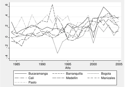
The analysis of the evolution of wage di¤erentials can be performed from di¤erent perspectives. To begin with, Figure 1 shows that during the …rst half of the sample period the public/private wage di¤erentials for male and female workers remain rel-atively stable. Then, during the second half of the sample period, these di¤erentials start to increase favouring the public sector. In addition, the public/private wage di¤erential for male workers does not appear to be statistically di¤erent from that of female workers. Notice that the previous analysis was undertaken at a very high level of aggregation, in the sense that we only looked at average wages in the public and private sectors by gender. However, the advantage of using survey data (as we do in this document) is that other additional dimensions can be exploited as well. In particular, we also calculate:

1. Average wage in the public and private sectors by city. Here we use the main seven metropolitan areas of the country that are available throughout the sample period; namely (in alphabetical order) Bucaramanga, Barranquilla, Bogotá, Cali, Medellín, Manizales and Pasto.

2. Average wage in the public and private sectors by gender and by city.

3. Average wage in the public and private sectors by occupational category. Here we consider the following four categories: managerial, professional, o¢ce and others.

4. Average wage in the public and private sectors by city and by occupational category.

appears to be closing. This …nding may be explained by the fact that Pasto exhibits a lower average wage in the private sector compared to other cities where smaller gaps are observed (as in the case of Bogotá). When one examines the gaps for male and female workers it is clear that the one for Pasto can be explained by the fact that the corresponding gap for men is wider than that observed for women; see Figures 3 and 4.

Figures 5 to 8 plot wage gaps by occupational position. These …gures illustrate an interesting …nding. While the public/private wage di¤erentials for managerial and professional employees (i.e. white collar employees) do not exhibit a signi…-cant variation, for the other two occupational positions (o¢ce and others) the wage di¤erentials show a slight increase.

Figures 9 to 22 summarise wage di¤erentials with respect to Bogotá. When using Bogotá as the category to which others are compared, the computed gaps do not show large changes over the sample period. Here there are two, somewhat expected, results that must be highlighted: (i.) wages in Bogotá are higher than in other cities; and (ii.) in the private sector the wage gaps with respect to Bogotá are much larger than those observed for the public sector.

Figure 23 compares the distribution of wages for the years 1985 and 2005. As can be seen from the …gure, the distribution of wages have not changed consider-able through time. An interesting …nding is that private sector wages appear more concentrated around the mean than public sector ones. When the data are further analysed by occupational categories, other interesting results emerge. The distrib-ution for managerial workers is very similar in the private and public sectors. For o¢ce workers the distribution of wages tends to be more concentrated, while for pro-fessionals and workers in managerial activities the wage distributions exhibit more variation around their respective means. On average, public sector wages tend to be higher than private sector ones.

also be observed when examining wage distributions across cities, perhaps with the exception of Pasto, where wages are found to be less concentrated. Medellín is the city with the largest concentration in wage distribution, and the largest mean in the private sector for 2005.

The previous results describe the behaviour of wages over time. However, for a better understanding of the size of wage di¤erentials is necessary to consider aspects such as human capital formation and demographic (market segmentation) factors. Thus, human capital formation appears in wage di¤erentials when looking at the occupational pro…le of an individual, while demographic factors appear when exam-ining di¤erences by gender or by city. In fact, interesting results are uncovered when one relates wage di¤erentials to age (as a proxy of an individual’s work experience), years of schooling, gender and occupational category.

In the case of the age, our results indicate that men have more experience for all occupational positions, although di¤erences in experience are smaller for blue collar employees. By sector, higher levels of experience are found in public sector workers, although in the case of white collar employees these di¤erences tend to be smaller. Important di¤erences in experience are also found within blue collar employees, which suggests that being an "o¢ce employee" or being another type of "blue collar employee" is determined by the educational level of the individual. The results just described provide the necessary justi…cation for studying the relationship between public and private wages at a more disaggregated level.

Thus far, the analysis of wage di¤erentials has been based on an informal vi-sual inspection of the resulting series. In the following section we provide a more formal statistical analysis to assess the time-series properties of the variables under consideration.

5

Empirical analysis

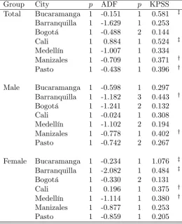
back-ground, an assessment of whether wages in these two sectors maintain a stable long-run equilibrium relationship can have implications for the necessity to adjust remuneration in the public sector. Hence, there is considerable value in understand-ing how public and private sector wages behave in relation to each other over time. Our analysis examines three di¤erent aspects of public/private sector wages. The …rst one is related to the time-series properties of the public/private wage di¤erential (Tables 1 and 2). The second one is concerned with the behaviour of public sector wages relative to that existing in Bogotá for an individual with similar character-istics (Tables 3 and 4). Lastly, the third one is related to the behaviour of private sector wages relative to that existing in Bogotá for an individual with similar char-acteristics (Tables 5 and 6). Thus, this sort of analysis allows us to examine wage di¤erentials existing between the public and private sectors, as well as those that arise within each of these two sectors.

the last autoregressive coe¢cient is statistically di¤erent from zero (say, at the 10% signi…cance level); if it is not statistically signi…cant, then the order of the autoregression is reduced by one until the last coe¢cient is statistically signi…cant. Then, we turn our attention to panel unit-root and panel stationarity tests. The main motivation for statistical testing using a panel of data instead of individual time series is that it has been noted that the power of the tests increases with the number of cross-sections in the panel. Thus, we …rst calculate the IPS test which tests the null hypothesis of a unit root in all individuals in the panel, and is based on the assumption of independence across individuals. Then, to allow for potential cross section dependence, we also calculate two additional tests: (i) the CIPS test for panel unit-root; and (ii.) the bootstrap Hadri panel stationarity test (the corresponding bootstrap p-values are based on 2,000 replications used to derive the empirical distributions of the test statistics). It should be recalled that failure to account for potential cross section dependence will result in severe size distortion of both the IPS and Hadri test statistics.

the 5% (but not at the 1%) signi…cance level; the resulting test statistics for all and female workers are 3.718 [p-value = 0.021] and 4.532 [p-value = 0.026], respectively. The reason why the CIPS and Hadri tests o¤er con‡icting results may be due to the fact that the wage di¤erentials are rather aggregate, as they do not discriminate by occupational category.

Table 2 reports the results for public/private wage di¤erential by occupational category and city. When the series are considered in isolation results tend to be con‡icting in the sense that both the ADF and KPSS tests either reject or fail to reject the null hypothesis. Panel tests, on the other hand, tell a completely di¤erent story. In this case, the CIPS test rejects the null hypothesis of joint non-stationarity for all occupational categories (i.e. managerial, professional, o¢ce and other), suggesting that at least one of the series in each panel is stationary. Stronger evidence in favour of stationarity is provided by the bootstrap Hadri test, as we fail to reject the null hypothesis of joint stationarity for any of the four occupational categories under consideration. These …ndings suggest that public and private sector wages maintain a long-run equilibrium relationship when analysed by occupational category, and after taking into account the presence of cross section dependence in the form of shocks (or innovations) that a¤ect all series simultaneously.

–2.210). Overall,the results support the view that wage di¤erentials are stationary. Table 4 presents the results for the case of the public sector wage di¤erential for the four occupational categories that are considered, with respect to the public sector wage of an individual in the same occupational category in Bogotá. As can be seen from the table, the results of the univariate unit-root and stationarity tests provide tend to favour the view that the wage di¤erentials are stationary, in particular when looking at the results of the KPSS test (where we fail to reject the null of stationarity in 20 out of 24 cases). Turning to the results of the panel tests, they also provide support that the public sector wage di¤erential with respect to Bogotá are stationary, with the exception of the CIPS test for individuals whose occupational category is "o¢ce".

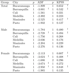
The last two tables relate to wage di¤erentials that involve the private sector. Table 5 shows the results when the tests are applied to private sector wages with respect to the wage of an individual with similar characteristics in the private sector in Bogotá. In this case the results of the univariate ADF and KPSS tests provide mixed evidence. However, the panel IPS, CIPS and Hadri tests provide support for the view that private sector wage di¤erentials with respect to Bogotá are stationary when considered as a panel of data. Indeed, while the IPS and CIPS reject the unit-root null hypothesis for the total population as well as for male and female workers, the Hadri tests fail to reject the null of stationarity.

6

Concluding remarks

In this document we have examined the time-series properties of the wage di¤eren-tials that arise between the public and private sector in Colombia. The analysis has been based on information taken from nationwide household surveys. The utilisation of survey data o¤ers the advantage that one can go beyond the typical calculation of the public/private sector wage di¤erential for male and female workers, as well as for all workers. Indeed, the data can be analysed at a very high level of disaggrega-tion. In particular, the dimensions that were studied in this document include: (i.) gender; (ii.) regional; and (iii.) occupational category.

Our …ndings indicate con‡icting results in the unit-root and stationarity tests when one focuses on wage di¤erentials at an aggregate level (such as for men, women and both). This is regardless of whether one is looking at each wage di¤erential in isolation of the others, or jointly as a panel of data.

Table 1. public/private wage di¤erential Univariate unit-root and stationarity tests

Group City p ADF p KPSS

Total Bucaramanga 1 -0.151 1 0.581 z

Barranquilla 1 -1.629 1 0.253

Bogotá 1 -0.488 2 0.144

Cali 1 0.884 1 0.524 z

Medellín 1 -1.007 1 0.334

Manizales 1 -0.709 1 0.371 y

Pasto 1 -0.438 1 0.396 y

Male Bucaramanga 1 -0.598 1 0.297

Barranquilla 1 -1.182 3 0.443 y

Bogotá 1 -1.241 2 0.132

Cali 1 -0.024 1 0.308

Medellín 1 -1.102 2 0.194

Manizales 1 -0.778 1 0.402 y

Pasto 1 -0.742 2 0.267

Female Bucaramanga 1 -0.234 1 1.076 z

Barranquilla 1 -2.082 1 0.484 z

Bogotá 1 -0.330 2 0.131

Cali 1 0.196 1 0.375 y

Medellín 1 -1.114 1 0.380 y

Manizales 1 -0.877 1 0.253

Pasto 1 -0.859 1 0.205

Panel unit-root and stationarity tests

Group IPS CIPS Hadri

Total 2.795 -3.040 z _3.718 z

Male 1.954 -3.490 z _2.218

Female 2.099 -2.930 z _4.532 z

Notes: _yand _zindicate 10 and 5% levels of signi…cance, respectively, based on critical

Table 2. public/private wage di¤erential by occupational category and city Univariate unit-root and stationarity tests

Occupational category City p ADF p KPSS

Managerial Bucaramanga 1 -2.389 3 0.159

Barranquilla 1 -1.407 1 0.330

Bogotá 1 -0.910 2 0.057

Cali 1 -3.356 z _{1 0.582} z

Medellín 1 -2.640 1 0.357 y

Manizales 1 -1.779 2 0.205

Pasto 1 -1.724 1 0.305

Professional Bucaramanga 1 -2.060 1 0.356

Barranquilla 1 -2.969 y _{1 0.256}

Bogotá 1 -1.964 1 0.314

Cali 1 -1.861 1 0.401 y

Medellín 1 -2.382 1 0.429 y

Manizales 1 -1.174 1 0.276

Pasto 1 -4.153 z _{1 0.415} y

O¢ce Bucaramanga 1 -0.812 2 0.156

Barranquilla 1 -0.572 2 0.193

Bogotá 1 -0.737 1 0.201

Cali 1 -0.244 1 0.197

Medellín 1 -1.587 1 0.328

Manizales 1 -0.475 1 0.216

Pasto 1 0.428 _y 0.254

Other Bucaramanga 1 -0.341 1 0.270

Barranquilla 1 -2.512 1 0.442 y

Bogotá 1 0.064 2 0.157

Cali 1 0.011 1 0.241

Medellín 1 -0.262 1 0.256

Manizales 1 -1.353 1 0.314

Pasto 1 -1.096 1 0.265

Panel unit-root and stationarity tests

Occupational category IPS CIPS Hadri

Managerial -1.421 y _-2.275 y _2.090

Professional -2.352 z _-3.015 z _3.298

O¢ce 2.613 -3.060 z _0.873

Table 3. Public wage relative to public wage in Bogotá Univariate unit-root and stationarity tests

Group City p ADF p KPSS

Total Bucaramanga 1 -3.741 z 1 0.223

Barranquilla 1 -3.048 z _{1 0.204}

Cali 1 -2.648 y _{1 0.223}

Medellín 1 -2.690 y _{1 0.118}

Manizales 1 -3.885 z _{1 0.157}

Pasto 1 -2.956 y _{1 0.155}

Male Bucaramanga 1 -4.441 z _{1 0.232}

Barranquilla 1 -2.968 y _{1 0.129}

Cali 1 -2.478 1 0.264

Medellín 1 -1.843 2 0.098

Manizales 1 -2.698 y _{1 0.158}

Pasto 1 -2.780 y _{1 0.237}

Female Bucaramanga 1 -3.046 z _{1 0.390} y

Barranquilla 1 -2.737 y 1 0.166

Cali 1 -3.012 y _{1 0.125}

Medellín 1 -3.356 z _{1 0.513} z

Manizales 1 -4.988 z _{1 0.813} z

Pasto 1 -3.051 z _{1 0.208}

Panel unit-root and stationarity tests

Group IPS CIPS Hadri

Total -4.214 z _{-2.082 0.100}

Male -3.462 z _{-2.035 0.211}

Female -4.735 z _{-2.149 3.397}

Table 4. Public wage relative to public wage in Bogotá by occupational category Univariate unit-root and stationarity tests

Occupational category City p ADF p KPSS

Managerial Bucaramanga 1 -3.238 z _{1 0.237}

Barranquilla 1 -2.281 1 0.347

Cali 1 -1.836 1 0.408 y

Medellín 1 -3.050 z _{1 0.350}

Manizales 1 -1.734 2 0.049

Pasto 1 -3.126 z _{1 0.310}

Professional Bucaramanga 1 -1.496 3 0.058

Barranquilla 1 -2.193 1 0.460 y

Cali 1 -3.265 z 1 0.214

Medellín 1 -2.294 1 0.101

Manizales 1 -3.415 z _{1 0.217}

Pasto 1 -2.080 1 0.372 y

O¢ce Bucaramanga 1 -4.421 z _{1 0.100}

Barranquilla 1 -1.918 1 0.058

Cali 1 -3.779 z _{1 0.177}

Medellín 1 -3.701 z _{1 0.118}

Manizales 1 -2.675 y 1 0.069

Pasto 1 -2.987 y _{1 0.090}

Other Bucaramanga 1 -2.865 y _{1 0.237}

Barranquilla 1 -4.222 z _{3 0.825} z

Cali 1 -1.634 1 0.081

Medellín 1 -1.527 1 0.172

Manizales 1 -1.840 1 0.271

Pasto 1 -1.904 1 0.249

Panel unit-root and stationarity tests

Occupational category IPS CIPS Hadri

Managerial -2.633 z _-2.592 z _1.906

Professional -2.410 z _{-1.946 1.093}

O¢ce -4.432 z _-2.324 z _-1.263

Other -2.090 z _-2.713 z _2.298

Table 5. Private wage relative to private wage in Bogotá Univariate unit-root and stationarity tests

Group City p ADF p KPSS

Total Bucaramanga 1 -1.809 1 0.652 z

Barranquilla 1 -3.001 y _{1 0.532} z

Cali 1 -1.561 1 0.331

Medellín 1 -2.392 1 0.223

Manizales 1 -2.525 1 0.417 y

Pasto 1 -1.932 1 0.127

Male Bucaramanga 1 -1.784 1 0.480 y

Barranquilla 1 -2.728 y _{1 0.494} z

Cali 1 -1.756 1 0.268

Medellín 1 -2.036 1 0.176

Manizales 1 -2.204 1 0.229

Pasto 1 -2.276 1 0.136

Female Bucaramanga 1 -2.113 1 0.607 z

Barranquilla 1 -3.624 z _{1 0.408} y

Cali 1 -1.686 2 0.296

Medellín 1 -3.674 z _{1 0.272}

Manizales 1 -2.950 y _{1 0.848} z

Pasto 1 -1.985 1 0.135

Panel unit-root and stationarity tests

Group IPS CIPS Hadri

Total -1.760 z -2.394 z 3.594

Male -1.574 y _-2.389 z _2.144

Female -2.961 z _-2.355 z _4.416

Table 6. Private wage relative to private wage in Bogotá by occupational category Univariate unit-root and stationarity tests

Occupational category City p ADF p KPSS

Managerial Bucaramanga 1 -1.793 1 0.227

Barranquilla 1 -0.946 2 0.093

Cali 1 -1.954 1 0.615 z

Medellín 1 -2.609 1 0.497 z

Manizales 1 -1.975 1 0.175

Pasto 1 -2.863 y _{1 0.284}

Professional Bucaramanga 1 -2.910 y _{1 0.134}

Barranquilla 1 -2.154 1 0.623 z

Cali 1 -2.212 1 0.503 z

Medellín 1 -2.426 1 0.297

Manizales 1 -2.330 1 0.649 z

Pasto 1 -2.203 2 0.127

O¢ce Bucaramanga 1 -2.929 y _{1 0.523} z

Barranquilla 1 -2.039 1 0.127

Cali 1 -1.718 1 0.428 y

Medellín 1 -3.286 z _{1 0.418} y

Manizales 1 -2.214 1 0.273

Pasto 1 -2.403 1 0.160

Other Bucaramanga 1 -1.956 1 0.126

Barranquilla 1 -2.516 1 0.119

Cali 1 -2.144 1 0.087

Medellín 1 -2.005 1 0.102

Manizales 1 -1.746 1 0.151

Pasto 1 -1.131 1 0.081

Panel unit-root and stationarity tests

Occupational category IPS CIPS Hadri

Managerial -1.299 y _-2.731 z _2.456

Professional -2.193 z _{-2.065 3.741}

O¢ce -2.345 z _-2.574 z _2.570

Other -1.025 -2.283 y _-1.103

Figure 1. Public/private sector wage di¤erential by gender

.4

.5

.6

.7

.8

.9

1985 1990 1995 2000 2005

Año

Male Female

Figure 2. Public/private sector wage di¤erential by city

.4

.6

.8

1

1.2

1985 1990 1995 2000 2005

Año

Bucaramanga Barranquilla Bogota

Cali Medellin Manizales

Figure 3. Male public/private sector wage di¤erential by city

.2

.4

.6

.8

1

1.2

1985 1990 1995 2000 2005

Año

Bucaramanga Barranquilla Bogota

Cali Medellin Manizales

Pasto

Figure 4. Female public/private sector wage di¤erential by city

.2

.4

.6

.8

1

1985 1990 1995 2000 2005

Año

Bucaramanga Barranquilla Bogota

Cali Medellin Manizales

Figure 5. O¢ce employees public/private sector wage di¤erential by city

.2

.4

.6

.8

1985 1990 1995 2000 2005

Año

Bucaramanga Barranquilla Bogota

Cali Medellin Manizales

Pasto

Figure 6. Other employees public/private sector wage di¤erential by city

0

.2

.4

.6

.8

1985 1990 1995 2000 2005

Año

Bucaramanga Barranquilla Bogota

Cali Medellin Manizales

Figure 7. Managerial employees public/private sector wage di¤erential by city

-.5

0

.5

1

1.5

1985 1990 1995 2000 2005

Año

Bucaramanga Barranquilla Bogota

Cali Medellin Manizales

Pasto

Figure 8. Professional employees public/private sector wage di¤erential by city

-.4

-.2

0

.2

.4

.6

1985 1990 1995 2000 2005

Año

Bucaramanga Barranquilla Bogota

Cali Medellin Manizales

Figure 9. Public sector wage di¤erential with respect to Bogotá

-.4

-.3

-.2

-.1

0

.1

1985 1990 1995 2000 2005

Año

Bucaramanga Barranquilla Cali

Figure 10. Public sector wage di¤erential with respect to Bogotá (male)

-.4

-.3

-.2

-.1

0

.1

1985 1990 1995 2000 2005

Año

Bucaramanga Barranquilla Cali

Medellin Manizales Pasto

Figure 11. Public sector wage di¤erential with respect to Bogotá (female)

-.4

-.2

0

.2

1985 1990 1995 2000 2005

Año

Bucaramanga Barranquilla Cali

Figure 12. O¢ce employees public sector wage di¤erential with respect to Bogotá

-.6

-.4

-.2

0

.2

1985 1990 1995 2000 2005 Año

Bucaramanga Barranquilla Cali Medellin Manizales Pasto

Figure 13. Other employees public sector wage di¤erential with respect to Bogotá

-.4

-.2

0

.2

.4

1985 1990 1995 2000 2005 Año

Figure 14. Managerial employees public sector wage di¤erential with respect to Bogotá

-1

-.5

0

.5

1

1985 1990 1995 2000 2005

Año

Bucaramanga Barranquilla Cali Medellin Manizales Pasto

Figure 15. Professional employees public sector wage di¤erential with respect to Bogotá

-.4

-.2

0

.2

.4

1985 1990 1995 2000 2005 Año

Figure 16. Private sector sector wage di¤erential with respect to Bogotá

-.8

-.6

-.4

-.2

0

1985 1990 1995 2000 2005 Año

Figure 17. Private sector wage di¤erential with respect to Bogotá (male)

-.8

-.6

-.4

-.2

0

1985 1990 1995 2000 2005 Año

Bucaramanga Barranquilla Cali Medellin Manizales Pasto

Figure 18. Private sector wage di¤erential with respect to Bogotá (female)

-.6

-.4

-.2

0

1985 1990 1995 2000 2005 Año

Figure 19. O¢ce employees private sector wage di¤erential with respect to Bogotá

-.6

-.4

-.2

0

.2

1985 1990 1995 2000 2005

Año

Bucaramanga Barranquilla Cali Medellin Manizales Pasto

Figure 20. Other employees private sector wage di¤erential with respect to Bogotá

-.8

-.6

-.4

-.2

0

1985 1990 1995 2000 2005

Año

Figure 21. Managerial employees private sector wage di¤erential with respect to Bogotá

-1

-.5

0

.5

1985 1990 1995 2000 2005 Año

Bucaramanga Barranquilla Cali Medellin Manizales Pasto

Figure 22. Professional employees private sector wage di¤erential with respect to Bogotá

-1

-.8

-.6

-.4

-.2

0

1985 1990 1995 2000 2005

Año

Bucaramanga Barranquilla Cali

Figure 23. Distribution of wages by occupational category

0

.5

1

1.5

2

0 5 10 15

Professional

0

.5

1

1.5

2

0 5 10 15

Managerial

0

.5

1

1.5

2

0 5 10 15

Office

0

.5

1

1.5

2

0 5 10 15

Other

Density

Private 1985

Public 1985

Private 2005

Public 2005

Figure 24. Distribution of wages by city

References

Adamchik, V. A. and A. S. Bedi (2000). Wage di¤erentials between the public and

the private sectors: Evidence from an economy in transition. Labour Economics 7,

203–224.

Alvarez, L. J., J. Jareño, and M. Sebastian (1993). Salarios públicos, salarios privados e in‡ación dual. Banco de España Working Papers from Banco de España No 9320.

Arango, L. E. and C. E. Posada (2002). Unemployment rate and the real wage behaviour:

A neoclassical hint for the Colombian labour market adjustment.Applied Economics

Letters 9, 425–428.

Arango, L. E. and C. E. Posada (2007). Los salarios de los funcionarios públicos en

colombia. Ensayos sobre Política Económica 55, 110–147.

Banerjee, A. and M. Wagner (2009). Panel methods to test for unit roots and

cointegra-tion. In T. C. Mills and K. Patterson (Eds.), Palgrave Handbook of Econometrics.

Volume 2: Applied Econometrics, pp. 632–726. Chippenham: Palgarve MacMillan.

Bender, K. A. (2002). The central government-private sector wage di¤erential. Journal

of Economic Surveys 12, 177–220.

Breitung, J. and M. H. Pesaran (2008). Unit roots and cointegration in panels. In

L. Mátyás and P. Sevestre (Eds.), The Econometrics of Panel Data, pp. 279–322.

Berlin: Springer-Verlag.

Campbell, J. Y. and P. Perron (1991). Pitfalls and opportunities: What

macroecono-mists should know about unit roots. NBER Macroeconomics Annual 6, 141–201.

Caner, M. and L. Kilian (2001). Size distortions of tests of the null hypothesis of

sta-tionarity: Evidence and implications for the PPP debate. Journal of International

Money and Finance 20, 639–657.

Carrión-i Silvestre, J. and A. Sansó (2006). A guide to the computation of stationarity

tests. Empirical Economics 31, 433–448.

Chang, Y. (2004). Bootstrap unit root tests in panels with cross-sectional dependency.

Journal of Econometrics 120, 263–293.

Dickey, D. A. and W. A. Fuller (1979). Distribution of the estimators for autoregressive

time series with a unit root. Journal of the American Statistical Association 74,

427–431.

Dickey, D. A. and W. A. Fuller (1981). Likelihood ratio statistics for autoregressive time

series with a unit root. Econometrica 49, 1057–1072.

Dustmann, C. and A. V. Soest (1998). Public and private sector wages of male workers

in germany. European Economic Review 42, 1417–1441.

Ehrenberg, R. G. and J. L. Schwarz (1986). Public sector labor markets. In O.

Ashenfel-ter and R. Layard (Eds.),Handbook of Labor Economics, Volume II, pp. 1219–1267.

Franses, P. H. (1998). Time Series Models for Business and Economic Forecasting. Cambridge: Cambridge University Press.

Fuller, W. (1976). Introduction to Statistical Time Series. New York, NY: Wiley.

Galvis, L. A. (2010). Comportamiento de los salarios reales en colombia: Un análisis de convergencia condicional, 1984-2009. Documentos de Trabajo sobre Economía Regional. Banco de la República. No 127.

Giulietti, M., J. Otero, and J. Smith (2009). Testing for stationarity in heterogeneous

panel data in the presence of cross section dependence. Journal of Statistical

Com-putational and Simulation 79, 195–203.

Granger, C. W. J. and P. Newbold (1974). Spurious regressions in econometrics.Journal

of Econometrics 2, 111–120.

Gregory, R. and J. Borland (1999). Recent development in public sector labor market.

In O. Ashenfelter and R. Layard (Eds.),Handbook of Labor Economics, Volume, pp.

3573–3630. Amsterdam: North Holland.

Hadri, K. (2000). Testing for stationarity in heterogeneous panels. The Econometrics

Journal 3, 148–161.

Hadri, K. and R. Larsson (2005). Testing for stationarity in heterogeneous panel data

where the time dimension is …nite. The Econometrics Journal 8, 55–69.

Hall, A. (1994). Testing for a unit root in time series with pretest data-based model

selection.Journal of Business and Economic Statistics 12, 461–470.

Hendry, D. F. (1980). Econometrics-alchemy or science? Economica 47, 387–406.

Hundley, G. (1991). Public- and private-sector occupational pay structures. Industrial

Relations: A Journal of Economy and Society 30, 417–434.

Im, K., M. H. Pesaran, and Y. Shin (2003). Testing for unit roots in heterogeneous

panels. Journal of Econometrics 115, 53–74.

Iregui, A. M. (2005). Decentralised provision of quasi-private goods: The case of colom-bia. Economic Modelling 22, 683–706.

Kwiatkowski, D., P. C. B. Phillips, P. Schmidt, and Y. Shin (1992). Testing the null

hypothesis of stationarity against the alternative of a unit root. Journal of

Econo-metrics 54, 159–178.

Lamo, A., J. Perez, and L. Schuknecht (2008). Public and private sector wages. co-movements and causality. European Central Bank. Working Paper Series. No 963.

Lora, E. and G. Márquez (1998). The employment problem in Latin America: Percep-tions and stylized facts. Inter- American Development Bank, Working Paper 371.

MacKinnon, J. G. (1991). Critical values for cointegration tests. In R. F. Engle and

C. W. J. Granger (Eds.), Long-Run Economic Relationships: Readings in

Cointe-gration, pp. 267–276. Oxford: Oxford University Press.