Revista Contaduría y Administración
Journal of Accounting and ManagementEditada por la División de Investigación de la Facultad de Contaduría y Administración de la UNAM
http:www.cya.unam.mx
Artículo original aceptado (en corrección)
Título: OLS Versus Quantile regression in extreme distributions
Autor: Moinak Maiti
Fecha de recepción: 29.09.2017
Fecha de aceptación: 16.05.2018
El presente artículo ha sido aceptado para su publicación en la revista Contaduría y Administración. Actualmente se encuentra en el proceso de revisión y corrección sintáctica, razón por la cual su versión final podría diferir sustancialmente de la presente. Una vez que el artículo se publica ya no aparecerá más en esta sección de artículos de próxima publicación, por lo que debe citarse de la siguiente manera:
OLS Versus Quantile regression in extreme distributions
Regresión OLS Versus Quantile en distribuciones extremas
Moinak Maiti1
Pondicherry University, India
Abstract
Financial data mostly have fat tail and an analyst is much concerned about the tail part. Most
of the study in finance extensible uses linear regression but when it comes to tail analysis it
becomes ineffective. So, the present study tries to address the same by using Quantile
regression in the tail analysis to study the value effect in 10 portfolios formed from BSE 500
stocks based on P/B ratio. The study result clearly indicates that Quantile regression estimates
give more comprehensive and vibrant picture of the unpredictable effect of the predictors on
the response variables.
Keywords: Quantile regression, decision making, factor models, Value effect
JEL Codes: C22, G11, G12
Resumen
OLS Versus Regresión cuantil en datos financieros extremos, en su mayoría tienen cola adiposa y un analista está muy preocupado por la parte de la cola. Más del estudio en finanzas extensible utiliza la regresión lineal, pero cuando se trata de análisis de la cola se vuelve ineficaz, Por lo tanto, el presente estudio trata de abordar el mismo mediante el uso de Quantile regresión en el análisis de cola para estudiar el efecto de valor en 10 carteras formadas a partir de BSE 500 acciones basadas en la relación P / B. El resultado del estudio indica claramente que las estimaciones de regresión de Quantile dar una imagen más completa y vibrante del efecto impredecible de los predictores en las variables de respuesta.
Palabras clave:Regresión cuantil; toma de decisions; modelos de factores y efecto Value
Codigos JEL: C22, G11, G12
1. Introduction
Most of the studies in finance has extensively used different factor model to understand the
risk return relationship. These factor models are generally linear in nature by linear it means
the dependent variable are linearly dependent on the independent variable. Financial data
generally have fat long tail and OLS regression at the end tails become ineffective. The
financial factor models are OLS regressions and OLS is based on the mean value of the
covariates and hence it is ineffective in the end distributions. Tail values are of more
significance to the analyst and risk managers as they have to make investment decision.
Decision based on OLS results mostly lead to wrong decision, to address the same Quantile
regression is used in evaluating these extremes of the distribution and compared with the OLS
results. In this paper 10 value sorted portfolios returns are analysed using the Fama-French
(1993) model using the OLS and Quantile regression methods exclusively to test value effect.
The paper is divided as follows section 2 of the paper deals with the review of literature
followed by the section 3 focus on the data & methodology that are used in the present study.
The empirical results and other calculations are shown in the Section 4 of the paper followed
by the discussion of the results in the section 5. Finally paper ends up with conclusions and its
implication to analyst for investment decision making.
2. Review of Literature
As earlier discussed most of the studies in finance extensively used OLS regression for
different factor models and none of the previous financial studies with factor models has
critically addressed whether the factor model is effective in capturing the tailed distribution
results or not? As in most cases the financial data consists of fat tails and in the tail part the
distribution generally do not follow normal curve distributions. Ordinary least square
regression follows the central tendency theorem and more effective at the median of the
distribution. Towards the extreme distributions it loses its effectiveness and due to which result
may not be correct. Embrechts, Kl¨uppelberg & Mikosch (1997) study used the extreme value
theory (EVT) and EVT then used for the extreme events analysis of floods, extreme
temperatures, winds and finance. Many researchers like Marinelli, D’Addona & Rachev
(2007), and Sheikh & Qiao (2009) have extensively used the extreme value theory to their
financial research to tackle the extreme events. For modelling two different methods namely
the block of maxima method and peaks over threshold method are used. Again there lies
some modelling technique to deal with this thick tails. Rachev (2003) in his book clearly
explains about the heavy tail distributions in finance and the difficulties associated with it. Then
it discussed about some probabilistic and statistical models like non-Gaussian to overcome
such problem. Recent study by David, Abhay and Robert (2011) and Dutta & Biswas (2017)
study confirms that financial tail data need special attention. It is clear that financial data do
have fat tails and over the period of time different researchers has followed different
methodology to overcome it but unable to capture as a whole.
Most of the studies in finance only use factor model or regression techniques. So, there are
possibilities that the study result has error especially at the end distributions. These are few of
the notable studies where the researchers have raised several questions regarding the factor
model usage in the financial studies. Fama-French results were tested by the Black (1993) and
the study finds that the size effect is due to the data mining effect rather than what is quoted in
the study. Kothari, Shanken and Sloan (1995) find that different frequency of data yield
different result for the beta effect and it is more prominent for the annual data. Similar result
also finds by the Levhari and Levy (1977) study that beta coefficients do differs for the annual
and monthly data. Kenz and Ready (1997) study find after trimming the 1 % tailed data using
the least trimmed squared techniques (LTS) the size effect greatly reduced. From all of the
above studies and several other studies that are not mentioned provides sufficient evidences
about the stocks returns move off from normality and shows fat tail distribution. The size effect
is also not constant for whole study period. For the present study uses the more vigorous
method of Chan and Lakonishok (1992).
3. Data and Methodology
Data
The present study uses monthly data of the BSE 500 stocks for the period from Jan 2003 to
April, 2015. Stock returns are calculated from the adjusted closing share prices of stocks.
Market capitalisation (MC) is used as the proxy for size and Price to book ratio (P/B) is used
as the proxy for value. BSE-200 index monthly excess return taken as the proxy for market
returns and all of the above mentioned data are collected from the Bloomberg database. 91day
T-bill returns are used as the proxy for the risk free rate of return (Rf) and it is collected from
the database of Reserve Bank of India (RBI).
10 weighted portfolios (each 10 %) are constructed by P/B ratio sort using the single sorting
techniques (Portfolios are named as Low, 2 to 9 and High). Mimi kicking portfolios are
constructed using the Fama-French (1993) methodology using both the single and double
sorting techniques as explained below. SMB2 and LMH3 (LMH used instead of HML in FFTF
regression, see Sehgal, S., Subramaniam, S., & De La Morandiere, L. P. (2012)) are mimicking
portfolio for size and value factors. By single sorting technique two value weighted market
capitalisation (MC) portfolio of ratio 90:10 are constructed. Then using the double sorting
techniques six portfolios are constructed from the cross of 2 size and 3 value sorted portfolios.
Portfolio S/L consists of small size and low P/B ratio companies; similarly Portfolio B/H
consists of big size and high P/B ratio companies; rest are named as S/M, S/H, B/L & B/M
based on acesending order of MC and P/B. Hence, every June moth of each year (t) portfolio
is ranked. Then each portfolios value weighted monthly excess return calculated for the period
of July, 2003 (t) to June, 2004 (t+1). In the similar process the next ranking done for the year
2004 and continues till 2015. Then for the whole period of 156 months from July, 2003 to
April, 2015, means excess returns on each portfolio are calculated. The formula for calculating
SMB and LMH are shown below:
SMB = (S/L + S/M + S/H)/3 − (B/L + B/M + B/H)/3 (1)
LMH = (S/L + B/L)/2 – (S/H + B/H)/2 (2)
Study uses Fama-French three factor models as discussed below:
RPt – RFt = a + b (RMt − RFt) + s SMBt + 𝑙 LMHt + et (3)
Where,
SMB mimics the risk factor in returns considering size
LMH mimics the risk factor in returns considering value
s and l are the portfolio’s responsiveness to (sensitivity coefficients) SMB and LMH factors
respectively.
Quantile regression
2 Small minus Big
Quantile regression is introduced by Koenker and Bassett (1978). It is based on the conditional
Quantile functions that estimate the conditional median or the conditional quartile of the
dependable variables for the given independent variables. It is quite similar to the OLS
regression as in OLS change in the coefficients of the independent variables denotes the change
from one unit change of the predatory variables associated with; in case of Quantile regression
it is the change of coefficients with changes in the specified Quantile from one unit change of
the predatory variables associated with it. Quantile divides the data into equal percentiles and
is more robust in capturing the outliers effectively. Quantile regression uses the median
estimator that reduces the sum of absolute errors to estimate the median function. Similarly for
other conditional Quantile function of interest (as in our case 0.05 and 0.95) is estimated by
reducing the asymmetric weight of absolute errors, where weights are function of the Quantile
for interest. In other words it can be said that Quantile are the optimization problem. Sample
mean can be defined as the solution to the problem of reducing the sum squares of residuals;
similarly the median can be defined as the solution to the problem of reducing the sum of
squares of absolute residuals with an aim to reduce the sum of square of residuals or absolute
errors. Sum of absolute residuals is said to be minimised when there is equal number of positive
and negative residuals lies above and below the median line. Similarly other quintile functions
can be obtained by giving different weights to the negative and positive residuals, i.e., by
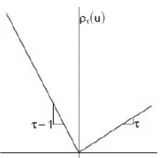
minimising the asymmetric weights of the residuals. In statistics or mathematical notations loss
function is defined as follows:
Ʈu if u > 0
ƍ
T=(Ʈ − 1)u if u ≤ 0
= u (Ʈ − I(u < 0)) (4)
The Ʈth quartile ξ minimises as shown in below equation (Univariate):
R (ξ) =∑𝑛𝑖=1ƍT(Yi − 𝜉) (5)
The above function has bidirectional derivatives and is not differentiable:
R’(ξ+) = Lim(h0+) (R(ξ + h)-R(ξ))/h
= Lim(h0+) ∑ ƍT(y−ξ−h)−ƍT(y−ξ)
h 𝑛
𝑖=1
= ∑𝑛𝑖=1(𝐼(𝑦𝑖 ≤ 𝜉) − Ʈ) (6)
Left derivative
R’(ξ-) = Lim(h0+) (R(ξ - h)- R(ξ))/h
= Lim(h0+) ∑ ƍT(y−ξ+h)−ƍT(y−ξ)
h 𝑛
𝑖=1
= ∑𝑛𝑖=1(Ʈ − 𝐼(𝑦𝑖 < 𝜉)) (7)
At point ξ minimises the objective function if R’(ξ+) ≥ 0 and R’(ξ-) ≥ 0
Figure No. 1: Quantile regression
The optimised problem defined the unconditional Quantile above in the similar way the
conditional Quantile can be defined analogously by OLS as explained below.
[Y1, Y2……….Yn] is a set of random variable from it, we get
Unconditional population mean is estimated from equation no. 8. Then the parametric function
µ (x, β) replaces the scalar µ in the above equation, we get equation 9
R (µ) =∑𝑛𝑖=1ƍT(Yi − 𝜇 (x, β))2 (9)
Similarly conditional median function can be obtained by replacing the scalar variable ξ by the
parametric function ξ (xt, β) and by setting the Ʈth quantile as 1/2. Other condition functions
values can be obtained on replacing absolute values by
ƍ
T(*), we get as follows:R (ξ) =∑𝑛𝑖=1ƍT(Yi − 𝜉 (x, β))2 (10)
Further using linear programming the minimising problem can easily be solved by formulating
ξ (x, β) as linear parameters.
In several areas of economics and other sciences this method has been used extensible in past.
Some of the notable studies are done to investigate the wage structure (Bunchinsky and Leslie
(1997)); educational attainment (Eide and Showalter (1998)); earnings mobility (Eide and
Showalter (1999), Buchinsky and Hahn (1998)). Similarly in finance several notable studies
are done related to VaR and options (Engle & Manganelli (1999) and Morillo (2000)); CAPM
(Barnes & Hughes (2002)); Fama-French three factor model (David, Abhay and Robert (2011))
etc., extensively using the same methodology.
4. Explanatory variables
The table No. 1 below shows the descriptive statistics of all the variables. Weak value effect is
observed in the portfolio returns as shown below in table No.1. Investor those who are investing
in the portfolios based on P/B is certainly not going get very less value premium. Hence,
investor shouldn’t consider P/B as the best indicator to construct the portfolios. For portfolio
construction other measures like size, investment, profitability, liquidity etc., or a mix of these
variables can be considered.
Portfolios Mean Median Max. Min. Std. Dev. Skewness Kurtosis
Low 0.025 0.023 0.438 -0.299 0.092 0.297 2.682
2 0.024 0.031 0.474 -0.308 0.093 0.665 3.846
3 0.026 0.024 0.473 -0.279 0.097 0.385 2.522
4 0.024 0.025 0.427 -0.309 0.096 0.261 2.524
5 0.028 0.029 0.444 -0.290 0.095 0.337 2.459
6 0.027 0.024 0.425 -0.303 0.091 0.177 2.644
7 0.022 0.023 0.420 -0.276 0.087 0.176 2.797
8 0.026 0.028 0.467 -0.297 0.096 0.310 2.879
9 0.023 0.025 0.457 -0.301 0.096 0.274 2.581
High 0.026 0.032 0.488 -0.286 0.094 0.525 2.877
Rm 0.006 0.004 0.318 -0.276 0.075 -0.093 3.680
SMB 0.025 0.016 0.221 -0.177 0.064 0.334 3.078
LMH -0.007 -0.009 0.262 -0.403 0.061 -1.243 3.461
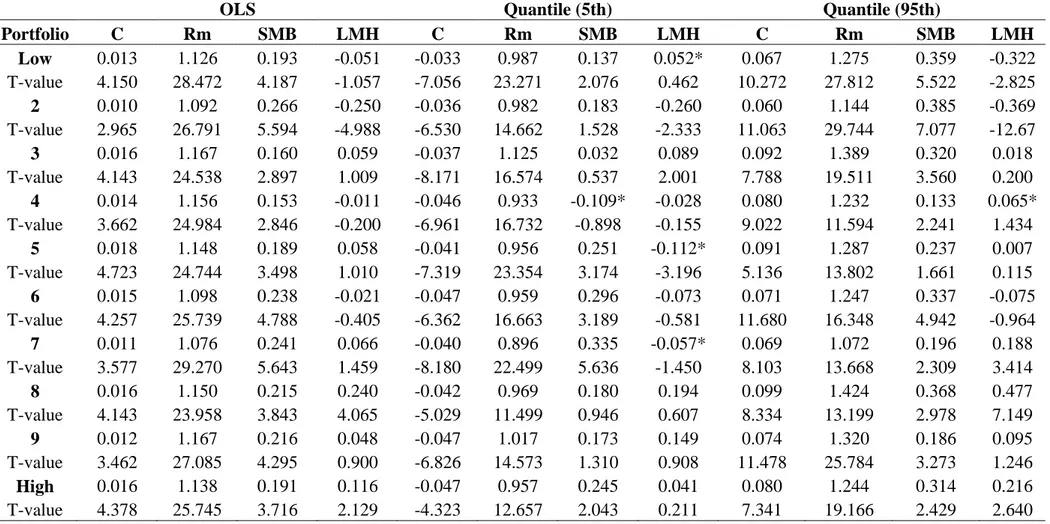
5. Empirical results
Below in table No.2 shows Fama-French Three factor coefficients obtained from both OLS
and Quantile regression (5th Quantile & 95th Quantile). OLS result shows all SMB coefficient positive whereas the coefficient obtained from Quantile regression at 0.05 Quantile shows
negative coefficient for portfolio number 4. That implies that at the lower quartiles relationship
between size and return is negative but it becomes positive in the higher quartiles. Hence, one
will make wrong decision if the decision is based on OLS regression only. Similar result
observed for portfolio number 4 in case of LMH coefficient where OLS result shows negative
coefficient for LMH but LMH coefficient obtained from Quantile regression at 0.95 Quantile
is positive. Here it implies that at the lower quartiles relationship between value and return is
positive but it becomes negative in the higher quartiles. Further the study result find similar
such observations and that are shown by * in the table No. 2. This clearly evidences the fallacy
OLS Quantile (5th) Quantile (95th)
Portfolio C Rm SMB LMH C Rm SMB LMH C Rm SMB LMH
Low 0.013 1.126 0.193 -0.051 -0.033 0.987 0.137 0.052* 0.067 1.275 0.359 -0.322
T-value 4.150 28.472 4.187 -1.057 -7.056 23.271 2.076 0.462 10.272 27.812 5.522 -2.825
2 0.010 1.092 0.266 -0.250 -0.036 0.982 0.183 -0.260 0.060 1.144 0.385 -0.369
T-value 2.965 26.791 5.594 -4.988 -6.530 14.662 1.528 -2.333 11.063 29.744 7.077 -12.67
3 0.016 1.167 0.160 0.059 -0.037 1.125 0.032 0.089 0.092 1.389 0.320 0.018
T-value 4.143 24.538 2.897 1.009 -8.171 16.574 0.537 2.001 7.788 19.511 3.560 0.200
4 0.014 1.156 0.153 -0.011 -0.046 0.933 -0.109* -0.028 0.080 1.232 0.133 0.065*
T-value 3.662 24.984 2.846 -0.200 -6.961 16.732 -0.898 -0.155 9.022 11.594 2.241 1.434
5 0.018 1.148 0.189 0.058 -0.041 0.956 0.251 -0.112* 0.091 1.287 0.237 0.007
T-value 4.723 24.744 3.498 1.010 -7.319 23.354 3.174 -3.196 5.136 13.802 1.661 0.115
6 0.015 1.098 0.238 -0.021 -0.047 0.959 0.296 -0.073 0.071 1.247 0.337 -0.075
T-value 4.257 25.739 4.788 -0.405 -6.362 16.663 3.189 -0.581 11.680 16.348 4.942 -0.964
7 0.011 1.076 0.241 0.066 -0.040 0.896 0.335 -0.057* 0.069 1.072 0.196 0.188
T-value 3.577 29.270 5.643 1.459 -8.180 22.499 5.636 -1.450 8.103 13.668 2.309 3.414
8 0.016 1.150 0.215 0.240 -0.042 0.969 0.180 0.194 0.099 1.424 0.368 0.477
T-value 4.143 23.958 3.843 4.065 -5.029 11.499 0.946 0.607 8.334 13.199 2.978 7.149
9 0.012 1.167 0.216 0.048 -0.047 1.017 0.173 0.149 0.074 1.320 0.186 0.095
T-value 3.462 27.085 4.295 0.900 -6.826 14.573 1.310 0.908 11.478 25.784 3.273 1.246
High 0.016 1.138 0.191 0.116 -0.047 0.957 0.245 0.041 0.080 1.244 0.314 0.216
T-value 4.378 25.745 3.716 2.129 -4.323 12.657 2.043 0.211 7.341 19.166 2.429 2.640
Table No. 2: Fama-French Three factor coefficients obtained from OLS and Quantile regression (5th Quantile & 95th Quantile)
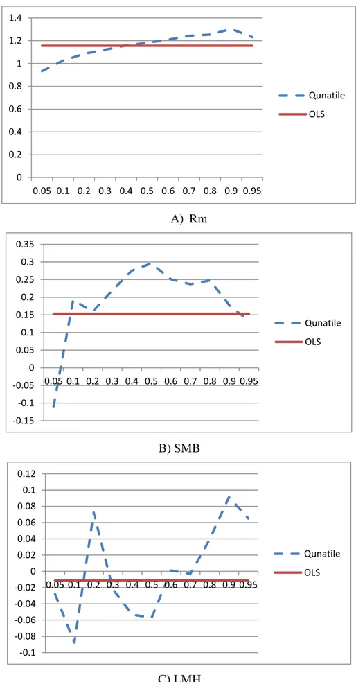
A) Rm
B) SMB
C) LMH
Figure No.2: Coefficient obtained from OLS and Quantile regression for Rm, SMB and
LMH for Portfolio 4. 0 0.2 0.4 0.6 0.8 1 1.2 1.4
0.05 0.1 0.2 0.3 0.4 0.5 0.6 0.7 0.8 0.9 0.95
Qunatile OLS -0.15 -0.1 -0.05 0 0.05 0.1 0.15 0.2 0.25 0.3 0.35
0.05 0.1 0.2 0.3 0.4 0.5 0.6 0.7 0.8 0.9 0.95
Qunatile OLS -0.1 -0.08 -0.06 -0.04 -0.02 0 0.02 0.04 0.06 0.08 0.1 0.12
0.05 0.1 0.2 0.3 0.4 0.5 0.6 0.7 0.8 0.9 0.95
Qunatile
Study result application and implications
From the above figure No. 2 it is clear that the value of the coefficient changes across the
Quantile. The value of the coefficient changes rapidly in between the quartiles and with
different frequency. For Rm the value of the coefficient increases with the higher Quantile. In
case of SMB the coefficient value is negative in the lower Quantile and it becomes positive at
the higher Quantile with difference in the frequencies across the Quantile. LMH coefficient
value changes much more frequently across the quartile and is much more complicated. So,
from the above graph it is clear that the OLS coefficient estimates only shows the average
relationship between the portfolio returns and the risk variables. OLS analysis implies that the
value of the coefficients is constant across the quintile which is really not the case as confirmed
from the figure No. 2. Further OLS coefficient estimates can only suggest the importance of
the anomalies but unable to predict “Does LMH (value) influences portfolio returns differently
for portfolios with low LMH than for average LMH?” Or “Does LMH (value) influences
portfolio returns differently for portfolios with average LMH than for high LMH”? But on the
other hand Quantile regression will state more comprehensive and clear picture of the effect of
the predictors on the response variables as clearly shown in the above figure No.2. Hence,
similar techniques can be replicated in other financial and economic studies where extensible
factor model or OLS is used to reduce the error in study results.
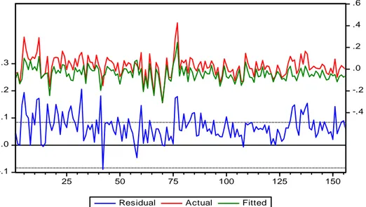
Model Prediction Performance test
The study uses residual graphs for model performance test as shown in the figure No. 3 below.
A) Residual graph obtained from OLS regression
-.2 -.1 .0 .1 .2
-.4 -.2 .0 .2 .4 .6
25 50 75 100 125 150
B) Residual graph obtained from Quantile Regression at 5th Quantile
C) Residual graph obtained from Quantile Regression at 95th Quantile
Figure No.3: Residual graphs obtained from the OLS and Quantile regression (0.05 & 0.95)
for portfolio 4
The residual graph shows the difference between the actual and fitted observation, value of
zero or closer to zero is better. From above figure No. 3 (A) residual graph of OLS regression
high peaks are observed hence OLS unable to capture all the values effectively. From figure
No. 3 (B) & (C) Quantile regression both at 0.05 & 0.95 Quantile able to capture all the values
as no peaks are observed. That justifies the supremacy of the Quantile regression over the OLS
particularly in the end distributions.
-.1 .0 .1 .2 .3
-.4 -.2 .0 .2 .4 .6
25 50 75 100 125 150
Residual Actual Fitted
-.3 -.2 -.1 .0 .1
-.4 -.2 .0 .2 .4 .6
25 50 75 100 125 150
Conclusion
The study starts with finding whether the 10 portfolios constructed from BSE 500 stocks based
on P/B shows any value effect in return patterns. The study find there exist a very weak value
effect in the return pattern of the P/B based portfolios. Further the study finds that the result
estimated by Quantile regression is more comprehensive and robust as compared to OLS result.
In many cases OLS shows positive/negative relationship between risk variables (Rm, SMB and
LMH) and returns but the Quartile regression estimators shows it is not consistent across the
Quantile. Hence, analyst or investment decision maker will get clearer picture about the risk
return relationship and can avoid heavy loss. Residual graph confirms the best fit for Quantile
regression result at the end tails. Hence, the study concludes that the Quantile regressions
estimates are better and more comprehensive than the OLS estimates at the end distributions.
The limitation of the study is that it is done in Indian context and hence in future one can test
the same using global data with more factors.
References:
Allen, D. E., & Powell, S. R. (2011). Asset Pricing, the Fama—French Factor Model and the
Implications of Quantile-Regression Analysis. In Financial Econometrics Modeling:
Market Microstructure, Factor Models and Financial Risk Measures (pp. 176-193).
Palgrave Macmillan UK.
Barnes, Michelle and Hughes, Anthony (Tony) W.,A Quantile Regression Analysis of the Cross
Section of Stock Market Returns(November 2002). Available at
SSRN:http://ssrn.com/abstract=458522
Black, Fischer, (1993)"Beta and Return," Journal of Portfolio Management 20 pp: 8-18.
Buchinsky, M., Hahn, J., (1998), “An alternative estimator for the censored quantile regression model”, Econometrica 66, 653-671.
Buchinsky, M., Leslie, P., (1997), Educational attainment and the changing U.S. wagestructure:
Some dynamic implications.Working Paper no. 97-13, Department 36 of Economics,
Brown University.
Chan, L.K. C. and J. Lakonishok, (1992) "Robust Measurement of Beta Risk", The Journalof
Financial and Quantitative Analysis, 27, 2, pp:265-282
Dutta, S., & Biswas, S. (2017). Extreme quantile estimation based on financial time
Eide, E. R., & Showalter, M. H. (1999). Factors affecting the transmission of earnings across
generations: A quantile regression approach. Journal of Human Resources, 253-267.
Eide, Eric and Showalter, Mark H., (1998), "The effect of school quality on student performance:
A quantile regression approach," Economics Letters, Elsevier, vol.58(3), pp:345-350,
Embrechts, P., C. Kl¨uppelberg and T. Mikosch (1997), Modeling extremal events for insurance
and finance, Springer.
Engle, R. F., & Manganelli, S. (1999). CAViaR: conditional value at risk by quantile
regression (No. w7341). National bureau of economic research.
Fama, E.F. and K.R. French (1993) Common Risk Factors in the Returns on Stocks and Bonds,
Journal of Financial Economics, 33, 3-56.
Kenz, P. J. and M. J. Ready, 1997, ‘On the robustness of size and book-to-market in cross-sectional regression’, Journal of Finance, 52, 1355-1382
Koenker, Roger W and Bassett, Gilbert, Jr, (1978), "Regression Quantiles," Econometrica,
Econometric Society, vol. 46(1), pages 33-50,
Kothari, S.P., Jay Shanken, and Richard G. Sloan, (1995), "Another Look at the Cross-Section of
Expected Returns," Journal of Finance, 50 (1995): 185-224.
Levhari, David, and Haim Levy, "The Capital Asset Pricing Model and the Investment Horizon,"
Review of Economics and Statistics, 59 (1977): 92-104.
Marinelli, C., S. D’Addona and S. Rachev (2007), ‘A comparison of some univariate models for
value-at-risk and expected shortfall’, International Journal of Theoretical and Applied
Finance 10(6), 1043–1075.
Morillo, Daniel. 2000. “Income Mobility with Nonparametric Quantiles: A Comparison of the U.S.
and Germany.”
Rachev, S.T. (editor) Handbook of Heavy Tailed Distributions in Finance. Elsevier, 2003
Sehgal, S., Subramaniam, S., & De La Morandiere, L. P. (2012). A search for rational sources of
stock return anomalies: evidence from India. International Journal of Economics and
Finance, 4 (4), 121-134.
Sheikh, A. Z. and H. Qiao (2009), ‘Non-normality of market returns: A framework for asset
allocation decision making’, Whitepaper, J.P. Morgan Asset Management, JPMorgan
Chase & Co .
Zumbach, G. (2006), ‘A gentle introduction to the RM2006 methodology’, RiskMetrics