C
C
|
E
E
|
D
D
|
L
L
|
A
A
|
S
S
Centro de Estudios
Distributivos, Laborales y Sociales
Maestría en Economía Universidad Nacional de La Plata
Estimating Income Poverty and Inequality from the
Gallup World Poll: The Case of Latin America and
the Caribbean
Leonardo Gasparini y Pablo Gluzmann
Estimating Income Poverty and Inequality
from the Gallup World Poll
The case of Latin America and the Caribbean
#Leonardo Gasparini * CEDLAS - UNLP
Pablo Gluzmann
CEDLAS – UNLP & CONICET
C | E | D | L | A | S **
Universidad Nacional de La Plata
This version: March 23, 2009
Abstract
This paper takes advantage of a new source of information – the Gallup World Poll 2006 – to estimate and characterize income poverty and inequality in Latin America and the Caribbean (LAC) at the country level, and to compare LAC statistics to those in other regions of the world. The Gallup survey has the advantage of being conducted in over 130 nations with almost the same questionnaire in all countries, and then it stands as a complement to national household surveys for international comparison purposes.
Keywords: povery, inequality, incomes, Latin America, Caribbean, Gallup
#
This study is a follow up of a large project commissioned by the IDB´s Latin American Research Network on Quality of Life in Latin America and the Caribbean, and carried out at CEDLAS with Mariana Marchionni, Sergio Olivieri and Walter Sosa Escudero. Gallup has generously provided the microdata of the Gallup World Poll 2006. We are grateful to Ravi Kanbur, Jere Berhman, Eduardo Lora, Carlos Vélez, Marcelo Neri, Carol Graham, Mauricio Cárdenas, Mariano Rojas, and seminar participants at the IDB (Washington D.C.), UNLP (La Plata), NIP (Córdoba) and LACEA (Rio de Janeiro) for helpful comments and suggestions. The usual disclaimer applies.
*
Corresponding author, leonardo@depeco.econo.unlp.edu.ar.
**
1. Introduction
The international comparison of income distributions has always been a central issue in Economics. Pareto (1897) produced one the first contributions in this field by comparing income distributions across European cities and states. Kuznets (1955) wrote a seminal paper comparing inequality across countries at different development levels. More recently, the international database of Gini coefficients of Deinenger and Squire (1996) and the World Development Indicators revitalized the empirical growth literature by adding inequality and poverty variables into the analysis.
Income poverty and inequality comparisons across countries and regions are usually carried out from household survey data. A first strand of the literature is based on aggregate distributional data (Gini coefficients, quintile shares) from secondary sources. This information is usually enriched with assumptions that allow estimating the shape of the whole distribution, and National Accounts GDP data to adjust the means. Bourguignon and Morrisson (2002), Bhalla (2002), Karshenas (2003) and Sala-i-Martin (2006) are examples of this literature. These contributions, although certainly very relevant, are naturally plagued by methodological problems, starting by the fact that the secondary distributional data comes from studies that use different well-being variables (income or consumption, net or gross income), have different coverage, have different units of analysis (individual or household) and are based on a very large number of methodological decisions that are not even documented in most papers (e.g. treatment of zero income, misreporting, outliers, regional prices, implicit rent from own housing, and so on).
A second strand of the literature makes comparisons based on household survey microdata, taking care of many of the problems mentioned above by applying a consistent methodology across surveys. This could be done at the regional level (see Gasparini, Gutiérrez and Tornarolli, 2007 for LAC), or with much effort at the world level. Ravallion and Chen (2008) is the last contribution of a series of papers from a World Bank project, in which income poverty around the world is computed from household survey microdata. Although they are careful in processing surveys in the same way, they allow different well-being variables in the dataset, and they recognize that “…there are problems that we cannot deal with. For example, it is known that differences in survey methods (such as questionnaire design) can create non-negligible
differences in the estimates obtained for consumption or income”. In a recent survey of
global income inequality Anand and Segal (2008) reach similar conclusions.
opportunity to compute alternative poverty and inequality statistics, and compare them with those obtained from household surveys.
This paper uses the Gallup World Poll to compute and characterize income poverty and inequality in Latin America and the Caribbean (LAC), and compare global statistics in that region with those in other regions of the world. The paper provides new results regarding poverty and inequality at the country level, and the position of LAC in the world ranking of these variables.
The rest of the paper is organized as follows. In section 2 we briefly describe the main sources of information for the study: the Gallup World Poll and the LAC national household surveys. Section 3 is aimed at discussing income measurement in the Gallup Poll. In section 4 we estimate levels and patterns of income poverty for all countries in the region based on Gallup data, and compare the results with those from household surveys. In section 5 we turn to income inequality, compute country and regional income disparities, and carry out some within-between decompositions. Section 6 closes with some concluding remarks.
2. The data
The main source of information for this study is the Gallup World Poll. During 2006, the Gallup Organization collected World Poll data using an identical questionnaire from national samples of adults from 132 countries, 23 of them from LAC. Sample sizes of 1,000 households per country were designed to assure national representativity. Because the survey has the same questionnaire in all the countries, it provides a unique opportunity to perform cross-country comparisons.1 The Gallup Poll includes basic questions on demographics, education, and employment, and a question on household income. The survey is answered only by an adult (15 or older) chosen randomly within the household.
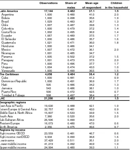
Table 2.1 shows some basic demographic statistics drawn from the 2006 Gallup survey, using population weights. The dataset includes the answers of 141,739 persons. 21,200 of them are inhabitants of LAC: 17,144 in Latin America and 4,056 in the Caribbean. The survey has full coverage in Latin America in terms of countries, and comprises the main nations in the Caribbean according to their population: Cuba, Dominican Republic, Haiti, Jamaica, Puerto Rico and Trinidad & Tobago. The country samples have around 1,000 observations, except in Haiti, Jamaica, Puerto Rico and Trinidad & Tobago, where around 500 observations were collected.
In some sections of this document we exploit the world coverage of the survey. In principle, this dataset provides a unique opportunity to study a wide range of issues with a true international perspective, since the samples are representative at the country level,
1
and the questionnaires are identical in all the countries. The last two panels in table 2.1 show some basic regional statistics, using two alternative standard classifications. Table 2.1 indicates that the share of males is lower but close to 50%, which is consistent with Census and household survey data. Naturally, mean age in the Gallup Poll is higher than in other sources, since respondents are older than 15. Although the correlation between mean age in the Gallup survey and in the household surveys is high (correlation coefficient=0.9), figure 2.1 shows some worrying differences for some countries (e.g. Guatemala and Paraguay). The mean number of children under 15 in the household reported in the Gallup Poll is somewhat higher than in household surveys: the LAC means are 1.5 and 1.34, respectively. The cross-country association in the number of children between Gallup 2006 and the national household surveys is statistically significant but not too tight (correlation coefficient=0.56).
Both Gallup and the LAC National Statistical Offices that conduct household surveys claim to work with samples that are representative at the national level. However, in reality the samples may well differ in their geographical coverage. In particular, the share of rural population may be different in the two sources, a fact that surely translates into differences in national statistics. We implement two definitions of urban from the Gallup data by alternatively classifying those who report living in a small town or village as urban (definition 1) or rural (definition 2) (see table 2.2). In some countries (e.g. Brazil) the (weighted) shares of urban observations in Gallup are similar to those reported in Census/surveys when using definition 1, while in others they seem to match official figures when using definition 2 (e.g. Chile, Costa Rica, El Salvador, Peru). In some other countries (e.g. Bolivia, Colombia, Paraguay) the “true” urban share (from surveys or Census) lies between the two alternative Gallup figures. In most cases where the household survey allows reclassifying observations and modifying the official definition of urban-rural, we can reasonably replicate the two alternative figures for the 2006 Gallup.2
In summary, a preliminary analysis suggests that basic statistics from the Gallup Poll are roughly consistent with those from household surveys in most LAC countries, but not in all, a fact that casts some doubts on the national representativity of the Poll in those countries. We return to this point in the next sections.
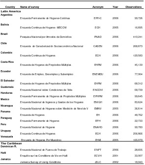
In addition to the Gallup Poll we use the national household surveys collected by the National Statistical Offices (NSO) of the LAC countries around 2006. Table 2.3 lists the surveys considered in this study. We use the datasets processed at CEDLAS as part of the SEDLAC project (Socio-Economic Database for Latin America and the Caribbean) carried out by CEDLAS and the World Bank's LAC Poverty Group (LCSPP), with the help of the MECOVI Program. The original microdata is processed using homogeneous definitions of variables, subject to the limitations imposed by the questionnaires.3
2
The exemptions are Jamaica and Venezuela. 3
see www.cedlas.org for details. Gasparini, Gutiérrez and Tornarolli (2007) use and discuss that data to
3. Income in the Gallup Poll
In spite of its drawbacks and limitations income adjusted by demographics is widely used as a proxy for individual well-being.4 In most countries poverty and inequality are officially measured over the distribution of income. This is certainly the case in LAC, where consumption data is seldom available in household surveys.
The Gallup survey includes a single question on monthly total household income before taxes. The question is clear, but it is too simple and reported in brackets, leading to just a rough measure of income. The question is placed almost at the end of the questionnaire, which may imply a higher rate of non response, and a lower quality of information. Additionally, the survey is conducted to a randomly selected member of the household (older than 15), not necessarily the person who knows the incomes of the household better.
The brackets of each question are expressed in local currency units (LCU), and hence they differ across countries, even when expressed in US$ adjusted for PPP. In fact, the number of brackets is different in each country. In the 2006 round in LAC, that number ranges from 4 in Colombia to 20 in Bolivia. In most countries (all in LAC) the question refers to monthly household income.
In all LAC countries we compute for each respondent an homogeneous monthly household income variable in US dollars by (i) randomly assigning a value in the corresponding bracket of the original question in LCU, and (ii) translating this value to US$ using country exchange rates adjusted for purchasing power parity (PPP). The assignment in step (i) is carried out by assuming that the shape of the income distribution in a given bracket of the Gallup Poll is similar to that of the national household survey, after adjusting for scale differences by multiplying Gallup figures for the ratio of median values of the two data sources. We apply this procedure only for LAC countries. When comparing this region with the rest of the world, we use an annual income variable standardized by Gallup, constructed by taking just the midpoints in each bracket (variable wp4898). For that reason, our statistics may differ when working either with LAC alone, or in comparison with the rest of the world.
Most welfare analysis are carried out in terms of household income adjusted for the demographic composition of the household. The Gallup Poll includes questions for the number of adults and children. However, unfortunately, the 2006 dataset includes the answers to the number of adults in only three LAC countries.5 In addition, the number of children is not recorded in Honduras and Nicaragua, and valid answers are less than 70% in Argentina and Mexico.
4
We estimate the number of members in each household by adding the number of children under 15 reported in the Gallup Poll to the average number of adults (above 15) computed from the national household surveys. For each country we take this average for four groups according to the area of residence (urban or rural), and the type of household (with or without children), and apply these means to the corresponding households in the Gallup survey. In addition, we estimate the number of children in households with missing information in Honduras, Nicaragua, Argentina and Mexico using data for the Gallup 2007 round.
Table 3.1 shows the mean, median and share of valid answers of total household monthly income, and per capita income for all LAC countries. The rate of income non-response is 14%, with maximum values in Trinidad and Tobago (39%) and Honduras (33%). On average (weighted by population) per capita income is 8% higher in the Caribbean. The unweighted average in the Caribbean is 59% higher: the main reason behind this difference is the relative low income in the highly-populated countries of Cuba and Haiti. The income dispersion in the Caribbean is very high. While mean monthly per capita income declared to Gallup is US$ 578 in Puerto Rico, it is just US$73 in Haiti. In Latin America the dispersion is lower: per capita income ranges from US$81 in Bolivia to US$321 in Chile.6
A likely measurement error in the Gallup Poll comes from the fact that the respondent is not necessarily the household head or spouse. Unfortunately, the 2006 dataset does not allow identifying the role of the respondent within the household. Therefore, in order to check for robustness of some results we compute statistics by dropping the answers of those respondents younger than a certain (variable) threshold. Results are robust to this change: for instance the linear correlation coefficient of per capita income for the whole sample and a sample where respondents younger than 30 are dropped is 0.99. Poverty and inequality changes do not significantly change either.
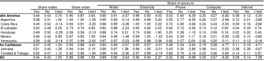
In table 3.2 the population is divided into those who answer the income question (column “yes”) and those who do not (column “no”), and compute several statistics for these groups separately. The analysis is restricted to those countries where income non-response is higher than 15%. If income non-non-response were random, the t-test of mean differences in the third column of each panel would be small. In most LAC countries that is in fact the case for the share of males and the urbanization rate. In contrast, in some countries (e.g. Argentina, Costa Rica) non-response seems to be concentrated in the well-off, as the access to phone, computer and Internet is significantly higher among those who refuse answering the income question. That is also true for the aggregate (Latin America, Caribbean and LAC). However, notice than in most countries the differences between the two groups are not statistically significant. Although there is certainly non-random income non-response in the Gallup Poll, at least in some
6
countries, the magnitude and the bias appear not to be very different from what is observed in household surveys (Gasparini et al., 2007).
Incomes in Gallup and household surveys
The national household surveys are the main sources of information on household incomes. These surveys usually include a relatively large number of questions aimed at capturing all sources of income. However, while household surveys are surely a better source for national income data than the Gallup Poll, the latter has the big advantage of a similar questionnaire across countries in the world, and hence it might compete with national surveys as a data source for international comparisons. In this section we compare the national income distributions drawn from the Gallup Poll to those obtained from the household surveys conducted by the National Statistical Offices of the LAC countries.
While the Gallup Poll was carried out in 2006, not all national surveys in our database correspond to that year (15 out of 20). To make the two information sources more comparable we take all incomes from the national household surveys to year 2006 by adjusting for the nominal income growth rate of each country (and thus implicitly assuming no distributional changes between the year of the survey and 2006).
We compute for each country non parametric estimates of the density function of the log per capita income in LCU from both sources of information.7 In general, incomes in Gallup are lower than in household surveys. When adjusting incomes for the difference in means the distributions are reasonably close in several countries. Figure 3.1 shows the comparisons between Gallup and household surveys for the whole region. Both distributions seem to match reasonably well in the case of Latin America, but not in the case of the Caribbean, where the Gallup distribution seems more egalitarian.
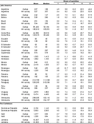
Table 3.3 adds to the analysis the estimates of mean and median per capita income in LCU in each country, along with the income shares by quintile. On average mean (median) income in Gallup is 57% (63%) of the value in national household surveys. Only in Jamaica and Venezuela incomes in Gallup are higher than in the household surveys. In most countries the shares of both the poorest and the richest quintiles are somewhat smaller than in household surveys.
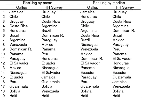
The linear correlation across countries between per capita income in Gallup and the national household surveys is positive, significant, not too high with the whole sample (0.61) but substantially high (0.95) when deleting the main deviants –Jamaica, Honduras and Venezuela- (see figure 3.2). When taking the medians the correlation coefficient are 0.58, and 0.93, respectively. The ranking across countries between the two information sources is similar (table 3.4). The Spearman rank correlation is 0.94 for the means and 0.88 for the medians when deleting the main deviants (panel B in table 3.4).
7
Incomes in Gallup and National Accounts
There are a host of reasons why mean income may differ between National Accounts (NA) and household surveys.8 Surveys record disposable incomes mostly from labor sources and transfers, while NA usually provide statistics on per capita GDP or consumption. Although the big facts (ranking of countries, growth rates) should in principle be similar regardless of the information source, that is not always the case: Gasparini, Gutiérrez and Tornarolli (2007) document significant differences in growth rates in LAC countries depending on the information source.
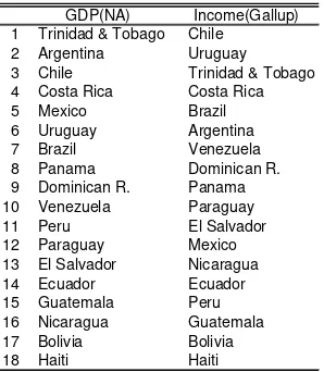
Figure 3.3 shows a reasonable degree of matching between mean income in Gallup and per capita GDP for the LAC countries. The linear correlation is 0.55 for the full sample, and raises to 0.83 when deleting the main outliers (Honduras and Jamaica). Table 3.5 shows the ranking of LAC countries according to both variables. Most nations are located in similar steps in the income ladder. Argentina and Mexico have mean incomes in the Gallup survey too low compared to their NA figures. The Spearman rank correlation coefficient is positive and significant (0.86).
Comparisons with the world
The Gallup survey allows comparisons across different regions in the world. According to Gallup microdata, income in LAC is higher than in sub-Saharan Africa, similar to South Asia, and lower than in the rest of the regions (see table 3.6).9 LAC mean per capita income is 13% of the value in North America, 21% in Western Europe, and 65% in Eastern Europe and Central Asia.10 These values imply some discrepancies with National Accounts figures, for which the income gaps between LAC and those regions are smaller.11 The main inconsistency arises in the comparison LAC-Asia: while according to Gallup data mean income is higher in East Asia and Pacific than in LAC, and it is just 12% higher in LAC than in South Asia, results drawn from other sources reveal substantial income gaps in favor of LAC.12
It is interesting to extend these comparisons to the whole income distribution. Figure 3.4 compares a non-parametric (kernel) estimation of the density function of the log per capita income in Latin America to that function in other regions of the world. Even after
8
See Deaton (2005). 9
Table 3.3 records annual income, not monthly income, as in previous tables. In addition, as our dataset includes incomes in LCU only for LAC countries, for world comparisons we use the rougher
standardization of income carried out by Gallup described above. 10
The rate of non-response for Middle East and North Africa is too high (89%), and the resulting mean income seems too high. Number of familiy members in Sub-Saharan Africa is not available in the dataset, so we cannot compute per capita income.
11
Per capita GDP (PPP) for 2006 in LAC was 22% of the value in North America, 30% in Western Europe, and 87% in Eastern Europe and Central Asia.
12
considering its drawbacks and limitations, the power of the Gallup survey is evident from graphs like 3.4. Several authors have tried to come up with comparable income distributions across regions. To that aim they use data from very different sources, and make a lot of assumptions. The Gallup data has the advantage of providing the necessary data for these estimations from the same question across more than a hundred countries.
The income distribution in Latin America seems close to that of the Caribbean. The Latin American distribution is located to the left of the distributions of both East Asia and Pacific, and Eastern Europe and Central Asia. The differences become more dramatic in the comparison with Western Europe and North America. In the next section we extend the analysis to some of the most socially relevant characteristics of the income distributions: poverty and inequality.
4. Income poverty
While the previous section deals with the whole income distribution, in this section we focus on measures of income poverty, i.e. the mass of the income distribution below certain threshold. There is a long-standing literature on the measurement of poverty. Even restricting the analysis to income poverty, the literature remains huge. The most widespread way of measuring poverty in an international context is by using the poverty lines set at US$1 or US$2 a day adjusted for PPP (Ravallion et al., 1991). Although these lines have been criticized, their simplicity and the lack of reasonable and easy-to-implement alternatives have made them the standard for international poverty comparisons.
The standard practice to get the international poverty lines in LCU is taking the equivalent to US$1.0763 in domestic currency using a large international study on prices carried out in 1993, and taking that value to the date of a given survey using the national consumer price index (Deaton, 2003; WDI, 2004). Table 4.1 shows several poverty measures obtained by applying the US$1 and US$2 lines to the distribution of household per capita income from the Gallup poll. Poverty statistics are shown for all countries for which we could compute poverty lines. According to these estimates the headcount poverty ratio in the region is 39.7% when using the US$2 line, and 18% when using the US$1 line. Poverty is higher in the Caribbean due to the presence of Haiti. Poverty ranges from 5.4% in Puerto Rico to 84.9% in Haiti (poverty line of US$2). In Latin America poverty ranges from 22.1% in Chile to 67.4% in El Salvador. Figure 4.1 shows the ranking of income deprivation: Puerto Rico, Trinidad & Tobago, the Southern Cone and Costa Rica have economies with relatively low income poverty levels, while some Andean and Central American countries are in the other extreme of the ranking.13 Haiti stands up as the country with the highest incidence of poverty in the region.
13
The main results do not change as we consider alternatively the US$ 1 or the US$ 2 lines, or the three poverty indicators -headcount ratio, poverty gap and FGT(2). In fact all the linear and rank correlation coefficients of the six columns in table 4.1 are statistically significant and high (higher than 0.95 in most cases).
Comparison Gallup and household surveys
The main sources for poverty estimates in LAC are the national household surveys. In this study we take the estimates of income poverty using the US$ 2 lines from our database at CEDLAS.14 For most countries we have poverty estimates based on microdata for 2006. For the rest we follow a procedure similar to the one described above: we assume neutral growth in per capita income (at the same rate as per capita GDP growth) from the year of the latest household survey available until 2006.
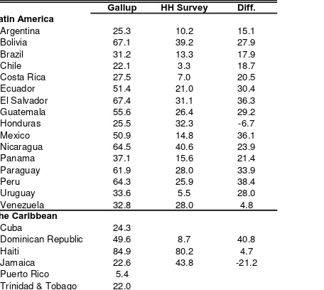
On average, poverty in the Gallup Poll is 16 points higher than in national household surveys when using the US$2 line. This gap is naturally linked to the differences in incomes between the two sources discussed in section 3. More than being concerned about the specific poverty levels that arise from the Gallup Poll, we care about the rankings and comparisons across countries, and across population groups within countries. Figure 4.2 shows a positive significant correlation between poverty estimates using the Gallup survey and those computed at CEDLAS with national household survey microdata. The linear correlation coefficient is 0.62 for LAC, 0.71 for Latin America, and 0.92 without the main income deviants identified in the previous section. The poverty ranking that arises from the two alternative data sources turns out to be similar (see table 4.3). The Spearman rank correlation coefficient is 0.93. Chile, Argentina, Costa Rica and Uruguay are the countries where income poverty is less serious, while Bolivia, Nicaragua and El Salvador are located in the other extreme.15 Haiti ranks as the country with the highest income deprivation level in the region. In summary, despite a much rougher approximation to per capita income, the picture of poverty in Latin America and the Caribbean viewed through the Gallup lens is not very different from the one obtained with household survey microdata. Poverty levels are highly correlated across both information sources and the poverty rankings are roughly consistent. However, there seems to be problems either with the national representativity of the survey or with the income variable in a few countries that should be revised and corrected in the next rounds of the Poll to increase the reliability and usefulness of the data.
Comparisons with the world
14
See www.depeco.econo.unlp.edu.ar/cedlas/sedlac for results and methodological details. 15
As commented above, there is a large and growing literature on international poverty comparison plagued by data comparability problems. The Gallup Poll provides an opportunity to alleviate some of these problems, since survey design and questionnaires are identical across countries.
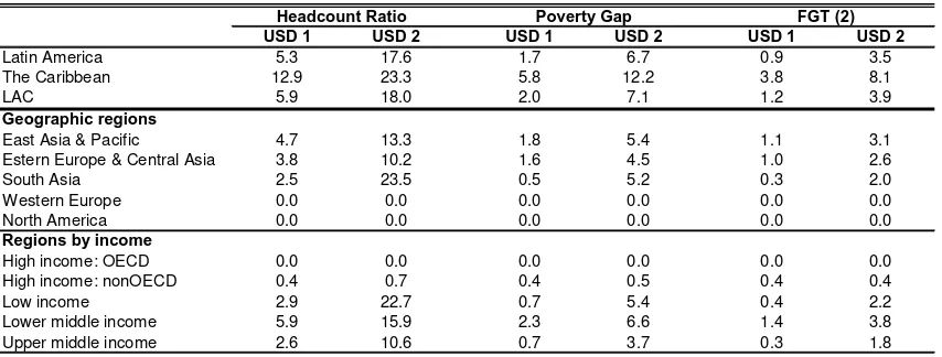
It is well known that poverty comparisons are sensible to the choice of the poverty line. Atkinson (1987) proposes checking for first-order stochastic dominance in order to assess the robustness of the results. In figure 4.3 we show the cumulated density functions for the income distribution in each region. Poverty in Latin America is lower than in the Caribbean, and higher than in East Asia and Pacific, and Eastern Europe and Central Asia.16 These results are confirmed in table 4.4.17 Poverty is almost inexistent in Western Europe and North America when measured with the US$1 or even the US$2 lines. As suggested by the overlapping distribution functions, the comparison LAC-South Asia is ambiguous. As mentioned above, this result seems unreliable according to other data sources.
5. Income inequality
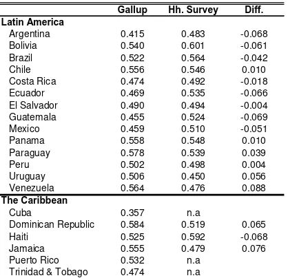
Latin America and the Caribbean has always been identified as a region with high levels of inequality. In this section we provide evidence on country and regional inequality with data from the Gallup Poll. We start by showing estimates of the most widespread indicator of inequality: the Gini coefficient for the distribution of household per capita income. In most countries income inequality is lower in the Gallup data than in the national household surveys (table 5.1), a fact that could be the consequence of a weaker income questionnaire in Gallup that misses some relevant income sources for the non-poor.18 More worrying are the differences in the inequality ranking among LAC countries (figure 5.1). Some countries which are consistently assessed as relatively egalitarian for the LAC standard look pretty unequal with the Gallup data (e.g. Uruguay, Venezuela). On the other hand, countries traditionally considered as very unequal are not ranked as so with the Gallup data (e.g. Haiti). The Spearman rank correlation coefficient of the Gini between estimates from Gallup and national household surveys is positive (0.354) but not statistically significant at 10%. The linear correlation is also positive (0.359) but weak (see figure 5.2).
There is a long standing debate on the economic performance of Cuba. Unfortunately, the government of that country has impeded the use of national statistics at the micro level, needed to make reliable international comparisons. Figure 5.1 is one of the few pieces of evidence of the presumably low level of income inequality in Cuba. Although
16
Ravallion and Chen (2008) find that poverty in LAC is higher than in Eastern Europe & Central Asia but lower than in East Asia & Pacific. Sala-i-Martin (2006) reports a ranking similar to that obtained with Gallup data.
17
For these comparisons we estimate incomes based on midpoints of the brackets in PPP US$ provided by Gallup. For that reasons estimates in tables 4.1 and 4.4 differ.
18
it is likely that the rank of Cuba in this graph reflects the true, the result should be still taken with prudence, given the discussions above and the concerns on the reliability of surveys in that country.
It has long been stated that Latin America is the most unequal region in the world. This proposition has been based on household survey microdata that differs in several dimensions across countries in different parts of the world. Although certainly plausible, the statement will remain debatable without comparable microdata. The Gallup Poll makes a contribution to this issue by providing income data using the same question in all the countries in the world.
There are two possibilities when analyzing inequality across regions in the world. The first one is to consider each region as a unit and compute inequality among all individuals in the region, translating their incomes to a common currency. In that alternative the division in countries of each region is completely ignored. The second alternative is to compute inequality in each region by taking an average of the inequality levels over the countries that form the region.
An assessment of inequality in the first sense (“within region inequality”) is presented in figure 5.3. The Lorenz curve of Latin America is clearly below those of Western Europe, North America, and Eastern Europe, but lies above those of East Asia and Pacific, and the Caribbean. The Gini coefficient of Latin America is 0.525 (see table 5.2), which is much higher than in Western Europe (0.402), North America (0.438) and Eastern Europe and Central Asia (0.497); but lower than in South Asia (0.534), the Caribbean (0.591), and Eastern Asia and Pacific (0.594). Table 5.3 shows that most results are robust to the choice of the inequality index. The exception is the comparison between LAC and South Asia, a fact that comes as no surprise, given the crossing of the Lorenz curves in figure 5.3.
Some of the results change when taking the second alternative to measure regional inequality; i.e. averages across countries (second column in table 5.2 and figure 5.4). Now, Latin America ranks as the most unequal region in the world, and the Caribbean looks less unequal. The cross-country Gini in Latin America (0.499) is only comparable to that of South Asia (0.489), and much higher than that of the Caribbean (0.456). To understand the difference in the results, notice that the dispersion in mean income is smaller in Latin America than in other regions like Eastern Asia and the Pacific, and the Caribbean. The Gini coefficient of the distribution of mean income across countries is 0.271 in Latin America, 0.401 in the Caribbean and 0.338 in East Asia and Pacific. While countries in Latin America are relatively similar in their stages of development, that is not true in the Caribbean or East Asia. In the Gallup Poll the income ratio between the poorest and the richest country is less than 5 in Latin America (Bolivia and Chile); more than 8 in East Asia and Pacific (Cambodia and Hong Kong), and more than 10 in the Caribbean (Haiti and Puerto Rico).
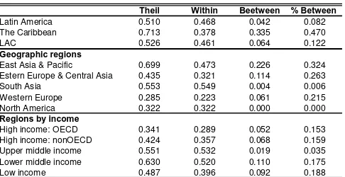
component in Latin America is relatively small compared to other regions in the world. Instead, in the Caribbean, one of the most diverse regions in the world, between inequality accounts for almost a half of total regional inequality.
Table 5.6 takes a brief look at world inequality by decomposing the global Theil, equal to 0.769, into a between and within components. It is interesting to note that almost half of the world income disparities can be accounted by differences across countries. This share is somewhat lower than the value estimated by Sala-i-Martin (2006), 64%, but still significantly large.
In a seminal paper Kuznets (1955) found evidence, and proposed an explanation, for an inverse-U relationship between inequality and development. Figure 5.6 makes a small contribution to the large and rich literature generated by that paper by showing a scatterplot of Gini coefficients drawn from the Gallup Poll and per capita GDP (in panel A) and per capita income (panel B). The relationship Gini-GDP seems to be decreasing. If we consider that the low-income African countries are not in the sample, the figure may not be inconsistent with the existence of a Kuznets curve. Panel B also shows a decreasing relationship between inequality and income per capita both measured with Gallup data.
It is interesting to note, in particular in panel A, that almost all the observations in Latin America lie above the curve. This is evidence in favor of the “Latin America´s excess inequality” documented in Londoño and Székely (2000), Gasparini, Cruces and Tornarolli (2009) and others: Latin American countries have high levels of income inequality, even after considering their levels of economic development.19
6. Concluding remarks
The Gallup World Poll constitutes a powerful instrument for international comparison of socio-economic variables. This paper exploits this dataset to study poverty and inequality in Latin America and the Caribbean, and to compare this region with the rest of the world.
We do not propose the use of the Gallup Poll as a subsitute for household surveys in distributional analysis, as the national surveys are substantially larger and richer. In fact, in the paper we point out some drawbacks and inconsistencies in the Gallup data that limit its use. However, at the same time, we highlight the enormous potential of the Gallup World Poll (or other similar surveys) for international comparisons of social statistics, if these drawbacks are overcame in the following rounds of the survey.
19
References
Anand, S. and Segal P. (2008). What do we know about global income inequality?
Journal of Economic Literature XLVI (1).
Bhalla, S. (2002). Imagine there’s no country: poverty, inequality and growth in the era
of globalization. Institute for International Economics, Washington DC.
Bourguignon, F. and Morrisson, C. (2002). Inequality among world citizens: 1820-1992
American Economic Review, 92(4): 727-744.
CEDLAS (2007). A Guide to SEDLAC. www.depeco.econo.unlp.edu.ar/cedlas/sedlac
Deaton, A. (1997). The analysis of household surveys. Microeconomic analysis for
development policy. Washington D.C.: The World Bank.
Deaton, A. (2005). Measuring poverty in a growing world (or measuring growth in a poor world). The Review of Economics and Statistics LXXXVII (1) February. Deininger, K. and Squire, L. (1998). New ways of looking at old issues: inequality and
growth. Journal of Development Economics 57(2), 257-285.
Gasparini, L., Gutiérrez, F. and Tornarolli, L. (2007). Growth and income poverty in Latin America and the Caribbean: evidence from household surveys. Review of
Income and Wealth, 53 (2), June.
Gasparini, L., Cruces, G. and Tornarolli, L. (2009). A turning point? Recent developments on inequality in Latin America and the Caribbean. Working paper UNDP and CEDLAS.
Gasparini, L., Marchionni, M., Olivieri, S. and Sosa Escudero, W. (2009). Multidimensional poverty in Latin America and the Caribbean. Manuscript, CEDLAS.
Karshenas, M. (2003). Global poverty: National Accounts based versus survey based estimates. Development and Change 34(4).
Kuznets, S. (1955). Economic growth and income inequality. American Economic
Review 45, 1-28.
Londoño, J. and Székely, M. (2000). Persistent poverty and excess inequality: Latin America, 1970-1995. Journal of Applied Economics 3 (1). 93-134.
Pareto, V. (1897). Cours d´èconomie politique. Pichon, Paris.
Ravallion, M., Datt, G. and van de Walle, D. (1991). Quantifying Absolute Poverty in the Developing World. Review of Income and Wealth 37.
Ravallion, M. and Chen, S. (2008). The Developing World Is Poorer Than We
Thought, But No Less Successful in the Fight against Poverty. Policy Research
Working Paper 4703. The World Bank.
Table 2.1
Basic demographic statistics Gallup World Poll 2006
Observations Share of Mean age Children males of respondent in the household Latin America 17,144 0.482 37.1 1.5
Argentina 1,000 0.480 41.0 2.0
Bolivia 1,000 0.498 35.6 1.9
Brazil 1,029 0.483 36.7 1.3
Chile 1,007 0.487 39.8 1.3
Colombia 1,000 0.479 37.2 1.4
Costa Rica 1,002 0.495 36.9 1.4
Ecuador 1,067 0.489 37.5 1.7
El Salvador 1,000 0.486 35.7 1.6
Guatemala 1,021 0.471 36.0 1.8
Honduras 1,000 0.486 34.1
Mexico 1,007 0.472 36.1 2.0
Nicaragua 1,001 0.485 34.7
Panama 1,005 0.502 37.2 1.5
Paraguay 1,001 0.473 37.5 2.0
Peru 1,000 0.496 37.7 1.7
Uruguay 1,004 0.474 43.3 1.0
Venezuela 1,000 0.490 36.5 1.5
The Caribbean 4,056 0.484 38.4 1.2
Cuba 1,000 0.481 41.3 0.9
Dominican Republic 1,000 0.491 36.9 1.7
Haiti 505 0.486 34.2 1.3
Jamaica 543 0.486 38.1 1.0
Puerto Rico 500 0.472 42.5 0.7
Trinidad & Tobago 508 0.497 38.4 0.7
LAC 21,200 0.482 37.2 1.5 Geographic regions
East Asia & Pacific 19,630 0.488 42.1 1.0 Estern Europe & Central Asia 32,757 0.481 42.0 0.9 Middle East & North Africa 15,837 0.533 33.9 1.5
South Asia 7,380 0.520 35.6 2.0
Sub-Saharan Africa 26,506 0.490 34.3
Western Europe 16,073 0.480 47.0 0.6
North America 2,356 0.475 46.6 0.7
Regions by income
High income: OECD 23,559 0.481 46.7 0.6 High income: nonOECD 9,934 0.490 36.8 1.6
Low income 37,429 0.511 35.1 2.0
Lower middle income 41,219 0.492 40.9 1.0 Upper middle income 24,994 0.480 39.3 1.1
Source: own estimates based on microdata from Gallup World Poll 2006.
Table 2.2
Share of urban observations Gallup World Poll 2006
Gallup Household
Def. 1 Def. 2 surveys Census Latin America
Argentina 99.9 85.9 Only urban 88.5 Bolivia 95.8 54.3 62.5 63.4 Brazil 81.8 72.8 82.8 82.2 Chile 99.0 84.3 86.6 86.3 Colombia 99.9 50.7 73.5 76.0 Costa Rica 84.1 55.5 59.0 60.0 Ecuador 97.6 60.0 66.3 63.9 El Salvador 72.0 53.7 59.7 62.4 Guatemala 94.8 36.1 45.5 40.3 Honduras 56.8 42.1 45.6 54.5 Mexico 83.6 67.3 76.6 74.8 Nicaragua 81.1 51.8 55.8 56.9 Panama 93.3 55.6 63.1 56.9 Paraguay 69.9 37.7 56.9 57.3 Peru 98.7 64.3 65.1 73.5 Uruguay 99.5 89.3 92.4 92.3 Venezuela 97.5 68.3 87.4
The Caribbean
Cuba 100 100 75.7 Dominican Republic 75.7 62.5 64.6 66.5 Haiti 70.7 50.4 40.6 37.0 Jamaica 94.8 37.8 44.1 57.1 Puerto Rico 54.2 40.6 75.9 Trinidad & Tobago 93.1 11.6 74.9
Source: own estimates based on microdata from Gallup World Poll 2006 and Census data.
[image:16.595.86.312.492.710.2]
Table 2.3
LAC household surveys used for this study
Country Name of survey Acronym Year Observations
Latin America
Argentina
Encuesta Permanente de Hogares-Continua EPH-C 2006 99,726
Bolivia
Encuesta Continua de Hogares- MECOVI ECH 2005 16,895
Brazil
Pesquisa Nacional por Amostra de Domicilios PNAD 2006 410,241
Chile
Encuesta de Caracterización Socioeconómica Nacional CASEN 2006 268,873
Colombia
Encuesta Continua de Hogares ECH 2006 120,583
Costa Rica
Encuesta de Hogares de Propósitos Múltiples EHPM 2006 45,139
Ecuador
Encuesta de Empleo, Desempleo y Subempleo ENEMDU 2006 77,964
El Salvador
Encuesta de Hogares de Propósitos Múltiples EHPM 2006 68,312 Guatemala
Encuesta Nacional sobre Condiciones de Vida ENCOVI 2006 68,739 Honduras
Encuesta Permanente de Hogares de Propósitos Múltiples EPHPM 2006 99,645 Mexico
Encuesta Nacional de Ingresos y Gastos de los Hogares ENIGH 2006 83,624 Nicaragua
Encuesta Nacional de Hogares sobre Medición de Nivel de Vi EMNV 2005 36,614 Panama
Encuesta de Hogares EH 2006 48,762 Paraguay
Encuesta Permanente de Hogares EPH 2006 22,733 Peru
Encuesta Nacional de Hogares ENAHO 2006 90,783 Uruguay
Encuesta Continua de Hogares ECH 2006 256,866 Venezuela
Encuesta de Hogares Por Muestreo EHM 2005 165,079
The Caribbean
Dominican R.
Encuesta Nacional de Fuerza de Trabajo ENFT 2006 28,655 Haiti
Enquête sur les Conditions de Vie en Haïti ECVH 2001 33,007 Jamaica
Jamaica Survey of Living Conditions JSLC 2002 18,943
Table 3.1
Monthly incomes in the Gallup survey Latin America and the Caribbean, 2006
Own estimates in US$ PPP from original questions
Total household income Per capita income
Mean Median % responses Mean Median % responses Latin America 703 487 0.86 174 109 0.85
Argentina 904 720 0.80 208 171 0.80
Bolivia 365 239 0.90 81 49 0.89
Brazil 754 524 0.96 209 130 0.96
Chile 1,333 733 0.87 321 176 0.85
Costa Rica 972 779 0.80 229 170 0.80
Ecuador 519 386 0.98 112 75 0.98
El Salvador 550 416 0.83 123 84 0.83
Guatemala 406 319 0.86 86 62 0.85
Honduras 1,029 976 0.67 213 200 0.67
Mexico 548 427 0.78 117 86 0.75
Nicaragua 647 537 0.81 113 95 0.79
Panama 588 397 0.97 138 82 0.97
Paraguay 657 423 0.96 135 71 0.90
Peru 478 360 0.87 101 69 0.87
Uruguay 918 661 0.93 275 178 0.93
Venezuela 738 468 0.82 166 91 0.81
The Caribbean 706 400 0.83 187 97 0.82
Cuba 463 442 0.93 124 114 0.93
Dominican Republic 693 401 0.85 162 86 0.83
Haiti 301 212 0.93 73 47 0.93
Jamaica 1,278 828 0.64 359 205 0.64
Puerto Rico 2,020 1,204 0.91 578 346 0.91 Trinidad & Tobago 962 735 0.61 273 190 0.59
LAC 703 477 0.86 175 108 0.85
Source: own estimates based on microdata from Gallup World Poll 2006.
Table 3.2
Variables by category of response to income question
Yes No t-test Yes No t-test Yes No t-test Yes No t-test Yes No t-test Yes No t-test Yes No t-test
Latin America 0.44 0.43 0.70 0.90 0.87 3.65 0.90 0.91 -0.57 0.96 0.93 4.03 0.53 0.60 -6.39 0.20 0.27 -6.82 0.08 0.12 -5.34 Argentina 0.38 0.31 1.92 1.00 1.00 -1.00 0.95 0.95 -0.14 0.99 0.99 0.20 0.55 0.77 -6.35 0.26 0.37 -2.99 0.12 0.21 -2.89 Costa Rica 0.49 0.50 -0.14 0.83 0.91 -3.20 0.96 0.99 -3.28 1.00 1.00 0.22 0.72 0.83 -3.65 0.24 0.43 -5.03 0.09 0.16 -2.69 El salvador 0.50 0.49 0.25 0.73 0.70 0.83 0.82 0.88 -2.23 0.93 0.92 0.42 0.60 0.72 -2.92 0.13 0.12 0.55 0.04 0.03 0.74 Honduras 0.49 0.50 -0.29 0.59 0.59 -0.10 0.88 0.74 5.31 0.74 0.69 1.90 0.25 0.28 -1.10 0.10 0.09 0.18 0.02 0.02 0.45 Mexico 0.46 0.42 0.90 0.87 0.83 1.59 0.94 0.96 -1.48 0.99 1.00 -1.33 0.54 0.50 1.17 0.18 0.21 -0.92 0.08 0.10 -0.89 Venezuela 0.39 0.40 -0.14 0.97 0.99 -2.62 0.97 0.97 -0.23 0.98 0.98 0.06 0.65 0.57 2.09 0.30 0.30 -0.11 0.11 0.12 -0.18
The Caribbean 0.47 0.45 1.24 0.83 0.88 -3.61 0.83 0.90 -5.07 0.95 0.97 -4.01 0.46 0.54 -3.64 0.19 0.28 -4.77 0.11 0.19 -4.71 Jamaica 0.51 0.45 1.28 0.94 0.94 0.19 0.99 0.97 1.38 0.99 1.00 -2.01 0.43 0.55 -2.86 0.38 0.41 -0.52 0.38 0.38 -0.07 Trinidad & Tobago 0.52 0.47 1.10 0.92 0.96 -1.94 0.89 0.94 -2.36 0.97 0.99 -2.19 0.69 0.70 -0.16 0.23 0.26 -0.80 0.14 0.11 0.97
LAC 0.44 0.43 1.05 0.89 0.88 1.93 0.89 0.90 -2.54 0.95 0.94 2.37 0.52 0.59 -6.99 0.20 0.27 -8.25 0.09 0.14 -7.28 Share males Share urban Water Electricity
Share of acces to
Internet Computer
Phone
Note: Column “yes” reports variables for those who respond the income question. Column “no” reports variables for those who do not answer the income question. The t-test assesses whether the difference between the two columns is statistically significant.
Only countries with rates of non response higher than 15%
[image:18.595.90.512.373.471.2]Table 3.3
Per capita incomes in PPP US$ Mean, median and share of quintiles
Estimates from Gallup and national household surveys
Share of quintiles
Mean Median 1 2 3 4 5
Latin America
Argentina Gallup 227 188 4.9 9.8 16.2 22.5 46.6 Argentina HH survey 527 357 3.4 8.2 13.6 22.0 52.8 Bolivia Gallup 242 147 2.5 7.3 12.1 20.2 57.9 Bolivia HH survey 539 286 1.8 6.2 10.9 19.6 61.6 Brazil Gallup 251 156 3.0 7.4 12.4 21.1 56.1 Brazil HH survey 534 295 2.6 6.6 11.2 18.7 60.9 Chile Gallup 95,426 52,184 3.0 6.6 10.9 18.9 60.5 Chile HH survey 180,810 105,851 4.2 7.8 11.8 18.7 57.5 Costa Rica Gallup 44,586 33,010 2.6 8.6 14.8 23.7 50.4 Costa Rica HH survey 103,015 65,462 3.9 8.4 12.8 20.1 54.8 Ecuador Gallup 60 40 4.2 9.1 13.5 21.0 52.2 Ecuador HH survey 138 82 3.6 7.6 11.9 19.1 57.8 El Salvador Gallup 63 43 3.5 8.3 13.7 21.0 53.5 El Salvador HH survey 121 83 4.6 9.2 13.8 20.7 51.7 Guatemala Gallup 395 287 3.9 9.3 14.8 21.9 50.1 Guatemala HH survey 974 579 3.5 7.3 12.0 19.2 58.1 Honduras Gallup 1,505 1,413 1.3 11.1 18.6 27.1 41.9 Honduras HH survey 1,862 1,100 2.3 6.7 12.0 20.0 59.0 Mexico Gallup 840 615 3.2 9.0 15.0 23.5 49.4 Mexico HH survey 2,418 1,520 3.7 8.2 12.7 19.7 55.6 Nicaragua Gallup 540 455 4.8 10.7 16.5 24.9 43.1 Nicaragua HH survey 1,220 743 3.8 7.7 12.2 19.2 57.0 Panama Gallup 89 53 1.7 6.3 11.9 21.4 58.6 Panama HH survey 182 105 2.5 6.8 11.7 20.1 58.9 Paraguay Gallup 213,709 111,538 2.0 5.5 10.7 20.9 60.9 Paraguay HH survey 539,205 315,036 3.0 7.1 11.8 19.1 59.0 Peru Gallup 139 96 2.8 7.8 13.8 22.0 53.6 Peru HH survey 366 237 4.0 8.0 13.0 20.7 54.3 Uruguay Gallup 2,879 1,860 3.3 7.4 13.0 21.6 54.7 Uruguay HH survey 6,474 4,406 4.6 8.8 13.7 21.4 51.6 Venezuela Gallup 298,695 163,116 2.0 7.0 11.2 19.5 60.2 Venezuela HH survey 280,529 194,157 2.8 8.6 13.9 21.8 52.9
The Caribbean
Dominican Republic Gallup 2,156 1,143 2.3 6.1 10.6 18.8 62.1 Dominican Republic HH survey 5,903 3,505 4.0 7.7 12.0 19.4 56.9 Haiti Gallup 1,077 692 2.7 7.8 13.2 20.3 56.0 Haiti HH survey 1,326 684 2.4 6.2 10.4 17.6 63.4 Jamaica Gallup 16,007 9,123 2.8 6.3 11.9 19.7 59.4 Jamaica HH survey 10,302 5,198 0.1 3.2 10.1 20.1 66.5
Table 3.4
Ranking of LAC countries
By mean and median values of household per capita income (US$ PPP)
A. All countries
Gallup HH Survey Gallup HH Survey
1 Jamaica Uruguay Jamaica Uruguay
2 Chile Chile Honduras Chile
3 Uruguay Costa Rica Uruguay Costa Rica
4 Costa Rica Argentina Chile Argentina
5 Honduras Brazil Argentina Dominican R.
6 Brazil Dominican R. Costa Rica Brazil
7 Argentina Paraguay Brazil Mexico
8 Venezuela Mexico Nicaragua Paraguay
9 Dominican R. Panama Venezuela Peru
10 Panama Peru Mexico Panama
11 Paraguay Honduras Dominican R. El Salvador
12 El Salvador Ecuador El Salvador Honduras
13 Mexico Nicaragua Panama Nicaragua
14 Nicaragua El Salvador Ecuador Ecuador
15 Ecuador Jamaica Paraguay Guatemala
16 Peru Guatemala Peru Jamaica
17 Guatemala Bolivia Guatemala Venezuela
18 Bolivia Venezuela Bolivia Bolivia
19 Haiti Haiti Haiti Haiti
B. Without main deviants
Ranking by mean Ranking by median
Gallup HH Survey Gallup HH Survey
1 Chile Uruguay Uruguay Uruguay
2 Uruguay Chile Chile Chile
3 Costa Rica Costa Rica Argentina Costa Rica
4 Brazil Argentina Costa Rica Argentina
5 Argentina Brazil Brazil Dominican R.
6 Dominican R. Dominican R. Nicaragua Brazil
7 Panama Paraguay Mexico Mexico
8 Paraguay Mexico Dominican R. Paraguay
9 El Salvador Panama El Salvador Peru
10 Mexico Peru Panama Panama
11 Nicaragua Ecuador Ecuador El Salvador
12 Ecuador Nicaragua Paraguay Nicaragua
13 Peru El Salvador Peru Ecuador
14 Guatemala Guatemala Guatemala Guatemala
15 Bolivia Bolivia Bolivia Bolivia
16 Haiti Haiti Haiti Haiti
Ranking by mean Ranking by median
Table 3.5
Ranking of LAC countries
By per capita GDP and per capita income from Gallup
GDP(NA) Income(Gallup) 1 Trinidad & Tobago Chile
2 Argentina Uruguay 3 Chile Trinidad & Tobago 4 Costa Rica Costa Rica 5 Mexico Brazil 6 Uruguay Argentina 7 Brazil Venezuela 8 Panama Dominican R. 9 Dominican R. Panama 10 Venezuela Paraguay 11 Peru El Salvador 12 Paraguay Mexico 13 El Salvador Nicaragua 14 Ecuador Ecuador 15 Guatemala Peru 16 Nicaragua Guatemala 17 Bolivia Bolivia 18 Haiti Haiti
Source: own estimates based on IMF and microdata from Gallup World Poll 2006.
Table 3.6
Annual incomes in the 2006 Gallup survey
Estimates in US$ PPP from Gallup standardized categorical variable
Total household income Per capita income
Mean Median % responses Mean Median % responses
Latin America 8,573 5,018 0.87 2,870 1,621 0.87
The Caribbean 8,136 4,615 0.83 2,999 1,558 0.83
LAC 8,542 4,979 0.87 2,879 1,617 0.86
Geographic regions
East Asia & Pacific 12,039 6,209 0.85 4,632 2,190 0.84
Estern Europe & Central Asia 11,509 7,586 0.83 4,461 2,827 0.79
Middle East & North Africa 35,728 30,770 0.11 13,623 12,008 0.11
South Asia 8,061 3,361 0.83 2,557 1,385 0.79
Sub-Saharan Africa 5,773 2,464 0.88
Western Europe 32,392 28,009 0.75 13,466 10,631 0.75
North America 55,820 42,526 0.91 21,932 15,744 0.91
Regions by income
High income: OECD 41,796 30,818 0.79 16,824 11,907 0.79
High income: nonOECD 31,683 21,229 0.55 12,444 8,127 0.55
Low income 7,575 3,336 0.86 2,666 1,430 0.32
Lower middle income 9,223 5,751 0.70 3,523 1,957 0.64
Upper middle income 11,178 7,110 0.75 3,957 2,333 0.68
[image:21.595.86.512.375.559.2]Table 4.1
Poverty in LAC from the 2006 Gallup survey
Poverty lines=US$1 and 2 a day
USD 1 USD 2 USD 1 USD 2 USD 1 USD 2
Latin America 18.0 39.7 8.6 18.7 5.8 12.1
Argentina 6.5 25.3 3.1 9.1 2.0 5.1 Bolivia 37.4 67.1 18.5 36.6 12.2 24.7 Brazil 12.1 31.2 5.7 13.6 4.0 8.4 Chile 7.0 22.1 2.1 8.4 1.0 4.3 Costa Rica 12.8 27.5 8.1 14.1 6.6 10.2 Ecuador 18.5 51.4 7.9 21.8 4.8 12.7 El Salvador 35.2 67.4 15.5 33.7 9.4 21.7 Guatemala 25.1 55.6 10.9 25.8 6.5 16.0 Honduras 18.0 25.5 13.9 18.0 12.7 15.3 Mexico 25.8 50.9 12.0 25.2 8.3 16.6 Nicaragua 31.2 64.5 12.8 31.2 7.7 19.3 Panama 18.5 37.1 11.1 19.3 8.8 13.8 Paraguay 40.5 61.9 21.0 36.9 13.9 26.4 Peru 35.7 64.3 17.5 34.2 11.1 23.1 Uruguay 13.0 33.6 4.7 14.4 2.4 8.1 Venezuela 16.5 32.8 9.7 16.7 7.3 11.9
The Caribbean 24.2 42.8 12.6 23.4 8.7 16.2
Cuba 10.9 24.3 6.7 11.6 5.3 8.2 Dominican Republic 26.4 49.6 11.8 25.0 7.2 16.2 Haiti 55.1 84.9 28.5 51.2 18.9 36.2 Jamaica 5.7 22.6 4.6 8.8 4.2 5.8 Puerto Rico 3.7 5.4 3.0 3.6 2.8 3.2 Trinidad & Tobago 7.4 22.0 3.5 9.8 2.6 5.9
LAC 18.4 39.9 8.9 19.0 6.0 12.4
FGT (2) Poverty Gap
Headcount Ratio
Source: own estimates based on microdata from Gallup World Poll 2006.
Table 4.2
Poverty in LAC from the Gallup survey and household surveys
Gallup HH Survey Diff. Latin America
Argentina 25.3 10.2 15.1 Bolivia 67.1 39.2 27.9 Brazil 31.2 13.3 17.9 Chile 22.1 3.3 18.7 Costa Rica 27.5 7.0 20.5 Ecuador 51.4 21.0 30.4 El Salvador 67.4 31.1 36.3 Guatemala 55.6 26.4 29.2 Honduras 25.5 32.3 -6.7 Mexico 50.9 14.8 36.1 Nicaragua 64.5 40.6 23.9 Panama 37.1 15.6 21.4 Paraguay 61.9 28.0 33.9 Peru 64.3 25.9 38.4 Uruguay 33.6 5.5 28.0 Venezuela 32.8 28.0 4.8
The Caribbean
Cuba 24.3
Dominican Republic 49.6 8.7 40.8 Haiti 84.9 80.2 4.7 Jamaica 22.6 43.8 -21.2 Puerto Rico 5.4
Trinidad & Tobago 22.0
[image:22.595.92.320.383.587.2]Table 4.3
Ranking of LAC countries by poverty Gallup and national household surveys
Gallup HH Survey
1 Haiti Haiti
2 El Salvador Nicaragua
3 Bolivia Bolivia
4 Nicaragua El Salvador
5 Peru Paraguay
6 Paraguay Guatemala
7 Guatemala Peru
8 Ecuador Ecuador
9 Mexico Panama
10 Dominican R Mexico
11 Panama Brazil
12 Uruguay Argentina
13 Brazil Dominican R.
14 Costa Rica Costa Rica
15 Argentina Uruguay
16 Chile Chile
Source: own estimates based on microdata from
[image:23.595.86.513.359.521.2]Gallup World Poll 2006 and national household surveys.
Table 4.4
Poverty in the regions of the world
USD 1 USD 2 USD 1 USD 2 USD 1 USD 2
Latin America 5.3 17.6 1.7 6.7 0.9 3.5
The Caribbean 12.9 23.3 5.8 12.2 3.8 8.1
LAC 5.9 18.0 2.0 7.1 1.2 3.9
Geographic regions
East Asia & Pacific 4.7 13.3 1.8 5.4 1.1 3.1
Estern Europe & Central Asia 3.8 10.2 1.6 4.5 1.0 2.6
South Asia 2.5 23.5 0.5 5.2 0.3 2.0
Western Europe 0.0 0.0 0.0 0.0 0.0 0.0
North America 0.0 0.0 0.0 0.0 0.0 0.0
Regions by income
High income: OECD 0.0 0.0 0.0 0.0 0.0 0.0
High income: nonOECD 0.4 0.7 0.4 0.5 0.4 0.4
Low income 2.9 22.7 0.7 5.4 0.4 2.2
Lower middle income 5.9 15.9 2.3 6.6 1.4 3.8
Upper middle income 2.6 10.6 0.7 3.7 0.3 1.8
Headcount Ratio Poverty Gap FGT (2)
Table 5.1
Inequality in Latin America and the Caribbean Gini coefficients, 2006
Gallup Hh. Survey Diff. Latin America
Argentina 0.415 0.483 -0.068 Bolivia 0.540 0.601 -0.061 Brazil 0.522 0.564 -0.042
Chile 0.556 0.546 0.010
Costa Rica 0.474 0.492 -0.018 Ecuador 0.469 0.535 -0.066 El Salvador 0.490 0.494 -0.004 Guatemala 0.455 0.524 -0.069 Mexico 0.459 0.510 -0.051
Panama 0.558 0.548 0.010
Paraguay 0.578 0.539 0.039
Peru 0.502 0.498 0.004
Uruguay 0.506 0.450 0.056 Venezuela 0.564 0.476 0.088 The Caribbean
Cuba 0.357 n.a
Dominican Republic 0.584 0.519 0.065
Haiti 0.525 0.592 -0.068
Jamaica 0.555 0.479 0.076 Puerto Rico 0.532 n.a
Trinidad & Tobago 0.474 n.a
Source: own estimates based on microdata from Gallup World Poll 2006 and national household surveys
Table 5.2
Inequality in the world
Regional Gini coefficients, within region and across countries
Within regions
Across countries
Latin America 0.525 0.499 The Caribbean 0.591 0.456 LAC 0.530 0.486
Geographic regions
East Asia & Pacific 0.594 0.471 Estern Europe & Central Asia 0.497 0.418 South Asia 0.534 0.489 Western Europe 0.402 0.340 North America 0.438 0.392
Regions by income
High income: OECD 0.448 0.358 High income: nonOECD 0.484 0.417 Low income 0.536 0.511 Lower middle income 0.558 0.464 Upper middle income 0.521 0.431
[image:24.595.87.304.400.573.2]Table 5.3
Inequality in the world By region
Gini CV Theil Decil 10/Decil 1 ATK e=0.5 ATK e=1 ATK e=2 GE(0) GE(2)
Latin America 0.525 1.316 0.510 34.2 0.225 0.390 0.614 29.316 0.866 The Caribbean 0.591 1.792 0.713 85.5 0.299 0.469 0.708 196.938 1.606
LAC 0.530 1.360 0.526 36.7 0.231 0.396 0.622 41.572 0.924
Geographic regions
East Asia & Pacific 0.594 1.685 0.699 61.5 0.292 0.494 0.819 0.726 1.420 Estern Europe & Central Asia 0.497 1.120 0.435 38.6 0.205 0.381 0.702 22.298 0.628 South Asia 0.534 1.551 0.553 22.4 0.233 0.391 0.572 17.107 1.203 Western Europe 0.402 0.886 0.285 14.9 0.133 0.250 0.449 0.288 0.393 North America 0.438 0.885 0.322 18.1 0.157 0.301 0.525 0.358 0.391
Regions by income
High income: OECD 0.448 0.946 0.341 18.8 0.161 0.301 0.511 0.358 0.448 High income: nonOECD 0.484 1.135 0.424 27.7 0.192 0.337 0.556 44.133 0.644 Low income 0.536 1.523 0.551 24.8 0.234 0.396 0.588 16.336 1.160 Lower middle income 0.558 1.700 0.630 49.6 0.261 0.448 0.790 9.422 1.445 Upper middle income 0.521 1.235 0.487 32.6 0.220 0.391 0.625 6.482 0.763
Source: own estimates based on microdata from Gallup World Poll 2006.
[image:25.595.85.512.117.239.2]CV=coefficient of variation. ATK (e) refers to the Atkinson index with a CES function with parameter e. GE(e) refers to the generalized entropy index with parameter e. GE(1)=Theil.
Table 5.4
Inequality by regions
Theil decomposition by country
Theil Within Beetween % Between
Latin America 0.510 0.468 0.042 0.082 The Caribbean 0.713 0.378 0.335 0.470 LAC 0.526 0.461 0.064 0.122
Geographic regions
East Asia & Pacific 0.699 0.473 0.226 0.324 Estern Europe & Central Asia 0.435 0.321 0.114 0.263 South Asia 0.553 0.549 0.004 0.006 Western Europe 0.285 0.223 0.061 0.215 North America 0.322 0.322 0.000 0.000
Regions by income
High income: OECD 0.341 0.289 0.052 0.153 High income: nonOECD 0.424 0.357 0.068 0.159 Upper middle income 0.551 0.532 0.019 0.035 Lower middle income 0.630 0.520 0.110 0.175 Low income 0.487 0.396 0.092 0.188
Source: own estimates based on microdata from Gallup World Poll 2006.
Table 5.5
Inequality in the world
Theil between-within decomposition
Within Beetween % Between
By Geographic regions 0.485 0.285 0.370 By Income Regions 0.449 0.315 0.412 By Countries 0.390 0.380 0.494
[image:25.595.87.330.330.455.2]Figure 2.1 Mean age
Gallup World Poll 2006 and household surveys
23 25 27 29 31 33 35 37
34 35 36 37 38 39 40 41 42 43 44
Mean age - Gallup
M
e
a
n
a
g
e
h
h
s
u
rv
e
ys
Paraguay
Guatemala
Figure 3.1
Density function of log per capita income Gallup and national household surveys Non parametric estimates
Not adjusting for scale differences Adjusting for scale differences
Latin America Latin America
The Caribbean The Caribbean
LAC LAC
0
.1
.2
.3
.4
-5 0 5 10
log pc income HHS Gallup Density of log p/c income
0
.1
.2
.3
.4
-5 0 5 10
log pc income HHS Gallup Density of log p/c income
0
.1
.2
.3
.4
-5 0 5 10
log pc income HHS Gallup Density of log p/c income
0
.1
.2
.3
.4
-5 0 5 10
log pc income HHS Gallup Density of log p/c income
0
.1
.2
.3
.4
-5 0 5 10
log pc income HHS Gallup Density of log p/c income
0
.1
.2
.3
.4
-5 0 5 10
log pc income HHS Gallup Density of log p/c income
Figure 3.2
Scatterplot mean and median of the distribution of per capita income (in US$ PPP) Gallup and national household surveys
Mean Median 0 100 200 300 400 500 600 700
0 50 100 150 200 250 300 350 400
Income - Gallup
In c o m e n a ti o n a l s u rv e y s 0 100 200 300 400
0 100 200 30
Income - Gallup
In c o m e n a ti o n a l s u rv e y s Venezuela Honduras Honduras Venezuela Jamaica Jamaica
[image:28.595.96.334.318.450.2]Source: own estimates based on microdata from Gallup World Poll 2006 and national household surveys.
Figure 3.3
Per capita GDP (PPP) - per capita income from Gallup
0 50 100 150 200 250 300 350 400
0 2000 4000 6000 8000 10000 12000 14000 16000 18000
GDP per capita (NA)
M e a n i n c o m e ( G a ll u p ) Jamaica Honduras
Source: own estimates based on IMF and Gallup World Poll 2006.
Figure 3.4
Density function of log per capita income Non parametric estimates
The Caribbean East Asia and Pacific Eastern Europe and Central Asia
South Asia Western Europe North America
0
.1
.2
.3
.4
2 4 6 8 10 12 log pc income
lat noa Density of log p/c income
0 .1 .2 .3 .4 .5
2 4 6 8 10 12 log pc income
lat weu Density of log p/c income
0 .1 .2 .3 .4 .5
2 4 6 8 10 12 log pc income
lat sas Density of log p/c income
0
.1
.2
.3
.4
2 4 6 8 10 12 log pc income
lat eca Density of log p/c income
0
.1
.2
.3
.4
2 4 6 8 10 12 log pc income
lat eap Density of log p/c income
0
.1
.2
.3
.4
2 4 6 8 10 12 log pc income
lat car Density of log p/c income
[image:28.595.91.509.511.731.2]Figure 4.1
Poverty headcount ratio Gallup Poll 2006
Poverty line=US$2 a day
0 10 20 30 40 50 60 70 80 90 P u e rt o R ic o T ri n id a d & T . C h ile C u b a A rg e n ti n a C o s ta R ic a B ra z il U ru g u a y P a n a m a D o m in ic a n R . M e x ic o E c u a d o r G u a te m a la P a ra g u a y P e ru N ic a ra g u a B o liv ia E l S a lv a d o r H a it i
Source: own estimates based on microdata from Gallup World Poll 2006.
Figure 4.2
Poverty headcount ratio
Line=US$2 a day
0 10 20 30 40 50 60 70 80 90
0 10 20 30 40 50 60 70 80 90 Gallup H o u s e h o ld s u rv e y s Honduras Jamaica Venezuela
[image:29.595.93.339.392.563.2]Figure 4.3
Distribution functions
Comparison Latin America with other regions in the world
The Caribbean East Asia and Pacific Eastern Europe and Central Asia
South Asia Western Europe North America
0
.2
5
.5
.7
5
1
0 10000 20000 30000 Household per capita income, US$ PPP
lat noa
0
.2
5
.5
.7
5
1
0 10000 20000 30000 Household per capita income, US$ PPP
lat weu
0
.2
5
.5
.7
5
1
0 10000 20000 30000 Household per capita income, US$ PPP
lat sas
0
.2
5
.5
.7
5
1
0 10000 20000 30000 Household per capita income, US$ PPP
lat eca
0
.2
5
.5
.7
5
1
0 10000 20000 30000 Household per capita income, US$ PPP
lat eap
0
.2
5
.5
.7
5
1
0 10000 20000 30000 Household per capita income, US$ PPP
lat car
Figure 5.1
The ranking of inequality in LAC Gini coefficient Gallup Household surveys 0.30 0.35 0.40 0.45 0.50 0.55 0.60 0.65 U ru g u a y V e n e z u e la A rg e n ti n a C o s ta R ic a E l S a lv a d o r P e ru M e x ic o D o m in ic a n R . N ic a ra g u a G u a te m a la E c u a d o r P a ra g u a y C h ile P a n a m a H o n d u ra s C o lo m b ia B ra z il H a it i B o liv ia 0.30 0.35 0.40 0.45 0.50 0.55 0.60 0.65 C u b a A rg e n ti n a M e x ic o E c u a d o r C o s ta R ic a T ri n id a d & T o b a g o E l S a lv a d o r P e ru U ru g u a y B ra z il H a it i P u e rt o R ic o B o liv ia J a m a ic a C h ile P a n a m a V e n e z u e la P a ra g u a y D o m in ic a n R .
Source: own estimates based on microdata from Gallup World Poll and national household surveys .
Figure 5.2
The Gini coefficient in Gallup and household surveys
0.40 0.42 0.44 0.46 0.48 0.50 0.52 0.54 0.56 0.58 0.60
0.40 0.42 0.44 0.46 0.48 0.50 0.52 0.54 0.56 0.58 0.60
Gallup H o u s e h o ld s u rv e y s
[image:31.595.91.353.554.701.2]