Unit roots and cycles in the main macroeconomic variables for Argentina

(1)

Raíces unitarias y ciclos en las principales variables

macroeconómicas de argentina

Jorge Eduardo Carrera

1

_{, Mariano Féliz}

2

_{y Demian Tupac Panigo}

3

Documento de Trabajo Nro. 20

Febrero 2000

1

CACES-UBA, UNLP 2

CACES-UBA, PIETTE-CONICET, UNLP 3

(2)

R

RA

A

Í

C

E

S

U

N

I

T

A

R

I

A

S

Y

C

I

C

L

O

S

E

N

L

A

S

P

R

I

N

C

I

P

A

L

E

S

V

A

R

I

A

B

L

E

S

M

A

C

R

O

E

C

O

N

Ó

M

I

C

A

S

D

E

AR

A

R

G

E

N

T

I

N

A

Jorge Eduardo Carrera1 (CACES-UBA, UNLP) Mariano Féliz2 (CACES-UBA, PIETTE-CONICET, UNLP) Demian Tupac Panigo3 (CACES-UBA, PIETTE-CONICET, UNLP)

First draft: August 1999. This version: January 2000.

Resumen

En este trabajo estudiamos las propiedades de integración de algunas de las principales variables macroeconómicas de Argentina. Presentamos una metodología robusta para el análisis de persistencia frente a los shocks que afectan a las variables macroeconómicas y sus consecuencias sobre la estimación del componente cíclico y del componente tendencial. Nuestra estrategia consisten en testear la estacionariedad de las series utilizando una secuencia de indicadores de forma de analizar el problema desde tres puntos de vista convergentes: Persistencia de las series, Raíz Unitaria y Raíz Unitaria con Quiebre Estructural, buscando obtener resultados robustos respecto a las propiedades de integración de 14 de las principales variables macroeconómicas argentinas.

De esta manera logramos clasificar a las series en cuatro grupos homogéneos de acuerdo con su orden de integración. Esto nos permite determinar la mejor estrategia a seguir para la estimación del componente cíclico de cada variable. Por ejemplo, encontramos que el PBI puede ser robustamente considerado como integrado de primer orden, I(1).

Keywords: Unit Root, Persistence, Cycles, Structural breaks, Argentinean

Macroeconomic variables

JEL Classification Numbers: C3, C5, E3

1_{jcarrera@isis.unlp.edu.ar} 2

mfeliz@inifta.unlp.edu.ar

3

(3)

U

UN

N

I

T

R

O

T

S

A

N

D

C

Y

C

L

E

S

I

N

T

H

E

M

A

I

N

M

A

C

R

O

E

C

O

N

O

M

I

C

V

A

R

I

A

B

L

E

S

F

O

R

AR

A

R

G

E

N

T

I

N

A

Abstract

In this paper we study the integration properties of some of the main macroeconomic series of Argentina. We present a robust methodology for the analysis of persistence of shocks affecting macroeconomic series and its consequences on the modeling of the cyclical and permanent components.

Our strategy consists on testing the stationarity of the series by using a sequence of indicators in such a way that we can analyze the problem from three converging points of view: Persistence of the series, Unit Root (UR) and UR with a Structural Breaks, thus reaching robust results regarding the integration properties of the main 14 Argentinean macroeconomic time series.

We are able to classify them in four homogenous groups according to its order of integration. This allows us to determine the best strategy for modeling the cyclical component of each variable. For example, we found that the GDP can be robustly considered integrated of order one, I (1).

Keywords: Unit Root, Persistence, Cycles, Structural breaks, Argentinean

Macroeconomic variables

JEL Classification Numbers: C3, C5, E3

6

(4)

U

UN

N

I

T

R

O

T

S

A

N

D

C

Y

C

L

E

S

I

N

T

H

E

M

A

I

N

M

A

C

R

O

E

C

O

N

O

M

I

C

V

A

R

I

A

B

L

E

S

F

O

R

AR

A

R

G

E

N

T

I

N

A

I. CYCLE, TREND AND THE DATA GENERATING PROCESS ... 1

I.A. DGP AND THE ORDER OF INTEGRATION... 2

I.B. SIMPLE MEASURES OF PERSISTENCE... 3

I.B.1. First order autocorrelation coefficient (FOAC). A recursive and rolling approach. ... 3

I.B.2. Relative persistence measure (RPM) ... 3

I.C. TEST OF UNIT ROOTS... 4

I.D. ROLLING AND RECURSIVE ADF TEST FOR UNIT ROOT... 5

I.E. VARIANCE RATIO MEASUREMENT (VR) ... 5

I.F. UNIT ROOT UNDER THE HYPOTHESIS OF A STRUCTURAL BREAK... 6

I.G. A SYNTHESIS OF THE DIFFERENT VIEWS... 8

I.H. THE METHODOLOGY... 9

I.I. THE DATA... 10

II. MEASURES OF THE PERSISTENCE OF THE MACROECONOMIC SERIES IN ARGENTINA ... 10

II.A. THE CYCLE... 10

II.B. WHAT CYCLE? ... 11

II.C. SIMPLE MEASURES OF PERSISTENCE... 11

II.C.1. First order correlation coefficients (FOAC)... 11

II.C.2. Relative persistence measure (RPM) ... 12

II.D. UNIT ROOT TESTS... 12

II.D.1. Augmented Dickey-Fuller (ADF) and Phillips-Perron (PP) ... 12

II.D.2. Recursive and Rolling Augmented Dickey-Fuller... 13

II.E. VARIANCE RATIO TEST (VR) ... 14

II.F. UNIT ROOT TESTS UNDER STRUCTURAL BREAK... 14

II.F.1. Perron unit root test with exogenous structural break... 14

II.F.2. Perron unit root test with endogenous structural break ... 15

III. A COMPARATIVE ANALISYS ... 16

IV. CONCLUSIONS ... 17

V. REFERENCES... 18

VI. FIGURES AND TABLES... 20

3

(5)

U

UN

N

I

T

R

O

T

S

A

N

D

C

Y

C

L

E

S

I

N

T

H

E

M

A

I

N

M

A

C

R

O

E

C

O

N

O

M

I

C

V

A

R

I

A

B

L

E

S

F

O

R

AR

A

R

G

E

N

T

I

N

A

I. C

YCLE

,

TREND AND THE DATA GENERATING PROCESS

The cycle is very important for macroeconomic theory and for economic policy. Since the 80s there has existed strong controversy as to whether the Real Business Cycle models are the most appropriate framework to explain the evolution of the economies. Thus there’s been dispute as to the role of real and monetary (nominal) shocks in the short and long run economic performance.

This relates to the fact that if shocks are mainly transitory then stabilization policies have a reason to be while if shocks are persistent the most appropriate policies are structural ones. The questions we consider relevant in this context and that we will try to answer (albeit partially) in this work centering our attention on the Argentinean economy are:

a) What is the importance and size of the cycle in Argentina for the most relevant series? b) What is the structure of shocks hitting the economy like? Are shocks transitory or

permanent? How persistent are they?

c) What is the best strategy to model the cycle in terms of the de-trending method to be used?

d) What is the effectiveness of stabilization policies?

e) Was the convertibility a structural change that modified the behavior of the series? f) How much does shock persistence matter to forecast the future behavior of a series? For any discussion on the cycle it is central to be able to measure it. That is, it is of great importance to define what is the actual object being studied. Different ways of measuring the cycle will give us very different estimations as regards its importance. As a matter of fact, it is possible that the cycle doesn’t exists at all (Cribari-Netto, 1996).

When we extract the cycle from a time series (yt) a first step is to determine which is the

permanent component (ypt) of the series and which is the cyclical one (Ct). The permanent

component is associated with the trend that the series is supposed to follow in the long run and the cycle with the stationary deviations. Thus the cycle is constructed as follows:

Ct = yt - ypt (1)

The fundamental problem appears when we need to establish the characteristics of the permanent component.

Till the appearance of Box and Jenkins (1970) methodology, stationary serially correlated deviations around a deterministic trend where the paradigm. Since then, attention has moved toward ARIMA4 models that allow working flexibly with any kind of series, being them stationary or not.

1

jcarrera@isis.unlp.edu.ar

2_{mfeliz@inifta.unlp.edu.ar} 3

dpanigo@bigfoot.com

4

(6)

This changed the way of determining and measuring the cycle since it meant moving from the generalized use of deterministic trends (in particular linear trends where the most common assumption when calculating the cycle) to stochastic trend specifications.

To be able to know what the most appropriate trend is, the first thing to do is to go back to the Data Generating Process (DGP). According to the structure of the DGP that best fits each series we’ll establish the kind of trend that should be used for each one. The DGP is thus crucial for the decomposition between trend and cycle and thus for the determination of the duration and amplitude of the cyclical fluctuations in each macroeconomic variable.

I.A. DGP and the order of integration

A series that needs to be differentiated k times to acquire stationarity is considered to be integrated of order k: I (k)

For example, a series as follows:

yt = α +ρyt-1 + εt (2)

given that ε is i.i.d., when ρ = 1 is non-stationary. This is known as a Random Walk with drift process5.

The series turns into a stationary one when it is differentiated (in the case of equation 2 only once), so the data generating process of this series is said to be a difference-stationary process (DSP).

This kind of series is also said to present stochastic non-stationarity (Charenza, 1997) and can be adequately modeled as a Unit Root process (URP) in the autoregressive terms. Nelson and Plosser (1982) in their pioneering work for the United States show that 13 of the 14 macroeconomic series they studied present stochastic non-stationarity, specifically that they are I (1), that is they have a stochastic trend and thus are to be modeled as Unit Root processes.

However, when the series is of the kind: yt = α + δt + εt with εi i.i.d.~N(0,σ

2

) (3)

yt is a stationary series around a deterministic trend. Stationarity is achieved when by

subtracting the deterministic component (in equation 3, α + δt) from yt. The process behind

this kind of series is called a trend-stationary process (TSP). This is an I (0) series, so it doesn’t need to be differentiated to make it stationary. This was the traditional way of treating series till Nelson and Plosser’s work came around. Maddala and Kim (1998) state that from the numerous empirical works in existence it is evident that the deterministic trend is most common amongst real rather than nominal variables.

In a TSP the effect of shocks vanishes in the long run when t moves farther away from the moment of the shock. With DSP the effect of the shock remains. This is what’s behind the idea of persistence of innovations.

A stochastic trend implies that each shock is permanent and changes the long run trend. Since the variance grows without limit, forecasting is made difficult in this kind of series, in comparison with trend-deterministic series where the variance is limited by the variance of errors and thus forecasting can be based on the trend.

A similar shock has different effects depending on whether the process is stationary or not; simplifying, I (0) or I (1). Then for a process where ρ= 1in period t we have:

yt = yt-1 + εt (4)

in t+1

yt+1 = yt + εt+1, substituting, we have: yt+1 = yt-1 + εt + εt+1 (5)

The effect of the shock in εt transports and persists in the following sub-periods indefinitely.

5

It should be noted that when yt is a RW with drift contains a deterministic trend. In (2) the constant α can be

interpreted as the deterministic trend. Suppose the value yt= y0 en t = 0; substituting repeatedly:

∑

=

+ +

= t

i i

t t y

y

1 0 ε

α with εi i.i.d.~N(0,σ 2

)

(7)

If the series is stationary I (0) with |ρ| < 1 in period t, we have:

yt = ρyt-1 + εt (6)

in t+1

yt+1 = ρyt + εt+1, substituting, we get: yt+1 = ρ 2

yt-1 + ρεt + εt+1 (7)

The effect of the shock slowly disappears, with greater velocity the lower the value of ρ. Then, shocks have no persistence so they can be considered transitory.

Another way of expressing the same is to state that the central distinction to determine whether the trend is stochastic or deterministic is to verify if the series returns to its deterministic trend (or mean in the case there is no trend), at least in a reasonable period of time. This, of course, relates to the persistence of innovations. An I (1) series is equivalent to the accumulation of shocks and no underlying force exists in the behavior of the series that will make it return to its mean systematically.

Making a mistake in the determination of the DGP could take to important errors. If the series is a TSP and we differentiate we are over-differentiating the series, and if the original series is a DSP and we treat it as a TSP when running the regression against time we are under-differentiating.

However, Plosser and Schwert (1978) state that the risk of over-differentiating is not as great if we analyze carefully the properties of the residuals of the regression. A central point, made by Nelson and Kang (1981), is that if the true data generating process is a DSP and we extract the trend treating it as a series with a TSP, then the cycle will exhibit spurious periodicity.

I.B. Simple measures of persistence

I.B.1. First order autocorrelation coefficient (FOAC). A recursive and rolling approach. The recursive methodology derived from Brown, Durbin and Evans (1975) consists in

estimating a parameter using sub-samples t = 1,....,k, for k = k0 ,...,T, where k0 is the start–up

value and T is the full sample size. Unlike recursive estimation, rolling parameters are computed using sub-samples that are a constant fraction δ0 of the full sample. In this way we

can keep constant the marginal weight of each observation.

Using this methodology we can obtain rolling and recursive estimations of the FOAC for each series yt which is calculated with the following expression:

T

y

k

T

y

r

_T t t T k t k t k t t k

∑

= + = − −

−

=

1 2 1

)

(

)

(

)

)(

(

(8)

where T is the rolling or recursive sample size, k is the number of lags (in this case equal to

1), and

(

)

1

k

T

y

T k t k t k

t

=

∑

−

+ = − −

In this way we can analyze the evolution of this simple measure both to build an ordinal classification of shocks persistence among the series and to evaluate its stability along time for the different cycle calculation methodologies.

I.B.2. Relative persistence measure (RPM)

This measure of persistence results from comparing the sum of the first six autocorrelation coefficient of the series with the ones of a series obtained as the average of 2000 Monte Carlo Simulation of random walk series without drift.

(8)

whereRW is an artificial random walk series,Xi_{is the i}th_{series (in log., stochastic cycle and}

deterministic cycle),

r

kRWand Xi k

r

are the k order autocorrelation coefficient for the RW and Xi

respectively.

If RPM indicator for a selected series are close to unity, no significant difference between this series and an I (1) variable exists.

When RPM>1, the series presents bigger shock’s persistence than a unit root process, so it is possible that it is an I (2) variable.

On the other hand, a RPM significatively lower than one is usually found in stationary variables.

I.C. Test of Unit Roots

Nelson and Plosser (1982) demonstrated that a time series has a stochastic trend if and only if it has a Unit Rood (UR) in the autoregressive component. In such a way, testing for the number of UR is equivalent to testing the existence of a stochastic trend.

Based on the fact that the parameter d in an ARIMA (p,d,q) 6 representation is equal to the number of Unit Roots, Dickey and Fuller constructed a test on the null hypothesis of UR. This is the so-called Dickey-Fuller (DF) test. Since it is based on the restrictive assumption of independent and identically distributed (i.i.d.) errors, several modifications of the test where developed allowing for some heterogeneity and serial correlation in errors. The most known and used are the Augmented Dickey-Fuller (ADF) test and the semi-parametric alternative of the (Modified) Phillips-Perron test (Phillips and Perron, 1988, for the original test and Perron and Ng, 1996, for the modified version of the test).

Nelson and Plosser used these tests, in the line of the original DF test. Sargan and Bhargava (1983) postulate a different approach presenting their test in a Durbin-Watson framework. Basically, the idea of the DF test is to check the null hypothesis of ρ = 1 in the following equation:

yt = α + ρyt-1 + εt (10)

The mechanism consists on testing the null of ξ=0 in the Ordinary Least Squares (OLS) regression in the following equation, which is equivalent to (10):

∆yt = α + ξyt-1 + εt (11)

where ξ= ρ - 1.

Rejection of the hypothesis ξ= 0 in favor of the alternative ξ< 0 implies that ρ < 1 and that yt

is integrated of order zero (0).

If we cannot reject ξ= 0, then we should repeat the test using ∆yt in place of yt. The

Dickey-Fuller equation changes to:

∆∆yt = ξ∆yt-1 + εt (12)

The tests based on the DF have different distributions for the null and alternative hypothesis. If yt is I (1), as indicated by the null hypothesis, then equation (11) represents a regression of

an I (0) variable on an I (1) one. In this case there is no limiting normal distribution. The distribution used is known as the Dickey-Fuller t distribution. Fuller (1976) tabulated the original critical values. MacKinnon (1991) and Cheung and Lai (1995) modified the critical values to take into account the effect of different sample sizes and number of lags.

For an acute critic on some of the problems of the tests based on the DF methodology see Maddala and Kim (1998).

One weakness of the DF test is that it doesn’t take into account the possible autocorrelation between errors εt. If this was the case, the OLS estimations in equation (11) or its substitutes

would not be efficient. The solution, implemented by Dickey and Fuller (1981), was to include as explanatory variable de lagged dependent variable. This solution is known as the Augmented Dickey-Fuller test (ADF).

Then, an equivalent equation to equation (11) is:

6

(9)

t t i k i t

t

y

=

ξ

+

Σ

ξ

∆

+

ε

∆

₋

=

− 1

1

1 (13)

The testing procedure is the same one as before and it is based on the t corresponding to the

ξ. The critical values are the same ones as those for the DF test.

Phillips (1987) and Phillips and Perron (1988) proposed a new test using a non-parametric correction for the presence of serial correlation. The objective was to eliminate the nuisance parameters on the asymptotic distribution caused by the presence of serial correlation in the errors εt.

This statistics are known as Zρ and Zt. For the case of an AR (1) without drift 7 : 2 1 1 2 2 2

)

(

2

1 )

1 ˆ

(

− −

_Σ

−

=

t T e

y

T

s

T

Z

_ρ

ρ

(14)

2 / 1 2 1 1 2 2 2 ˆ

)

(

)

(

2

1

− −

_Σ

−

=

t T e e t

y

T

s

t

s

S

Z

_ρ (15)

Cochrane (1991) remarked the low power of the Unit Root tests as well as of any other test where a null hypothesis of ρ=ρ0against the alternativeρ0-κwithκsmall for reduced samples.

Although the difference between ρ0 y ρ0-κ could be reduced and even insignificant from the

economic point of view, this is especially problematic in the case of Unit Root tests for there exists a discontinuity in the theory of distribution in vicinity of the unit root. Thus, in such cases, these tests would not answer the question of which is the most appropriate distribution for small samples.

I.D. Rolling and Recursive ADF test for Unit Root

Another alternative to test unit root consists in evaluating the shifting root hypothesis. For this purpose the recursive and rolling developed by Banerjee, Lumsdaine and Stock (1992) provides a complete set of analysis.

Applied to the Unit Root Hypothesis, the procedure consists in estimating rolling and recursively8 the maximum and minimum ADF t statistics and comparing them with the 5% asymptotic critical values. In addition, we analyze the difference between the maximum and minimum ADF statistics, which can be associated with a measure of shifting root or root volatility.

I.E. Variance ratio measurement (VR)

An alternative non-parametric instrument to evaluate the presence of a unit root is to measure the degree of persistence. Cochrane (1988) proposed such alternative.

Using Beveridge and Nelson’s (1981) decomposition we can see that each series can be modeled as a combination of a non-stationary random walk (RW) and a stationary component. However, the RW can have an arbitrarily low variance, so that the power of the UR tests is arbitrarily low for small samples.

Cochrane (1991) highlights the importance of measuring the size of the RW component through the degree of persistence of the shocks in the levels of the series.

The measurement presented by Cochrane (1988) is as follows:

)

var(

.

)

var(

1 1 − −

−

=

t t k t t k k

y

k

y

V

VR

(16)

If yt is stationary, then lim k_!∞ VRk=0 and if yt is a RW, VRk=1 for any lag size.

A direct estimation for VR is the following:

7

For the cases of an AR (1) with a drift, and with a drift and a linear trend see Maddala and Kim (1998).

8

(10)

∧

∧ ∧

=

t k k

VR

σ

2

(17)

In practice, several values for VRk are considered and the null is rejected if at least one of the

VRk generates evidence against it (Maddala and Kim, 1998).

I.F. Unit Root under the hypothesis of a Structural Break

The idea of a structural break is associated with changes in the parameters in a regression. Discussions on the constancy of parameters have been very rich in econometrics, with a great number of test developed with respect to the matter (for a review and classification see Maddala and Kim, 1998).

The point that we are interested in focusing on for this study is how structural changes can affect the results for the Unit Root tests.

A pioneering article on the subject was one by Perron (1989) where he argues that, in general, shocks are transitory and the series are sporadically hit by extraordinary (not regular) events. Since its probability distribution is different to that of other regular shocks, he proposes changing them from the noise component to the deterministic trend of the series. In other words, innovations are transitory (and so stationary) around a deterministic trend that can sporadically suffer changes of different kind (in the constant, in the slope, or both). Perron’s proposal is very strong and puts back into discussion what had consolidated as the dominant framework in the 80s on the existence of a stochastic trend in the majority of the economic time series. That is, that they were generated by a DSP.

For example, the existence of a structural break represented by a change in the value of the mean in a series could make the conventional analysis conclude that there exists a unit root when in reality none exists. It is just that the series was and is still stationary, but now around a new mean. Charenza and Deadman (1997) indicates that the most simple case of a stationary series I (0) that suffers a jump (structural break) in the mean in the middle of the sample could be described by a random walk with drift of the kind:

yt = α + ρyt-1 + εt (18)

with ρ = 19.

The conclusion is that the autoregressive equation could bias ρtowards 1. In this case, in the presence of a structural break, the tests of the Dickey-Fuller kind tend to accept the null hypothesis of a Unit Root when actually the process is stationary to both sides of the structural break.

Perron applies the test to Nelson and Plosser’s series and find that the hypothesis of Unit Root must be rejected in all of the series with the exception of the Consumer Price Index, the velocity of money and the nominal interest rate. For that reason, he considers that the majority of the series have a segmented linear trend.

From Perron’s work on, there has been a long sequence of tests that gained in complexity. In Perron (1989) he proposes a modified DF test for Unit Root in the noise function with three different alternatives for the deterministic trend function of the series (DTt).

In the first one he allows for a structural change reflected in the intercept (crash model).

Model A: DTt = α + βDUt + δt (19)

where a) DUt= 1 if t> Tb; 0 otherwise.

The second model only allows for a change in the slope (changing growth model).

Model B: DTt = α + δ0t + δ1DT*t (20)

where b) DT*t= t-Tb if t> Tb; 0 otherwise.

The third model gives place to changes both in the intercept and the slope.

Model C: DTt = α + βDUt + δ0t + δ1DT*t (21)

9

(11)

The strategy followed by Perron is to first de-trend the series and then analyze the behavior of the residuals. Perron then obtains the limit distribution with the Ordinary Least Squares of the normalized estimators of

ρ

ˆ

and the corresponding t-statistics of the following regression:

yt i

= ρiyt-1 + εt (22)

where: yt i

with i = A, B, C being the residuals of the regression of yt corresponding to each of

the models.

The test by Perron is a conditional test for a given structural break point, which is defined ex-ante. For this reason, it is criticized for the possibility of pre-testing bias.

Since this proposal, there have been several attempts to give endogeneity to the structural breaks by using recursive, rolling and sequential tests. The first two take sub-samples, from the general sample, that may grow or remain fixed (with a constant marginal weight for the new data points); meanwhile, the sequential test progressively increase the date of the hypothetical break by using different dummy variables.

The endogeneization of the structural break generated several papers that reverted previous Perron results, but when the existence of more than one endogenous structural break is allowed, the number of rejections of the UR hypothesis once again increases.

Perron (1993, 1994a, 1994b) and Volgelsang and Perron (1994) propose two models to allow for endogenous structural changes: Additive outliers (AO) model and Innovational outliers (IO) model.

The difference between the two models is in the way they understand the change. In the AO model the change is abrupt while in the IO change is gradual and is affected by the behavior of the noise function since it moves in a similar way as the shocks that affect this function (Cati, 1997).

For AO models the three kinds of structural changes seen before (A, B and C) are applicable while for the IO modes only A and C are. The B version in the IO models is not often used in empirical application because it is not easy to apply when using linear estimation methods. The AO model is performed using a two step regression procedure, for the case of change in the slope of the trend function when the segments are joined at the time break. The point is to test the t-statistics of ρ =1. Let DTt = t – Tb if t>Tb; and 0 otherwise with Tb the time of break.

The first step consists on estimating the following regression:

t t

t

DT

y

=

µ

+

β

+

γ

+

~

(23)

Later, the error term (

y

~

_t) is modeled as follows:

t j t j k

j t

t

y

c

y

=

ρ

+

Σ

∆

₋

+

ε

=

−

~

1

1 (24)

We can obtain the IO models analyzing them separately under the null and the alternative hypotheses.

In the first case (under the null), using Perron’s (1994) notation, we can describe model A as follows:

IO1, Model A1:

y

t

=

y

t−1

+

b

+

ψ

(

L

)(

e

t

+

δ

D

(

T

b

)

t

)

(25)

Similarly, the expression for Model C is:

IO2, Model C1:

y

t

=

y

t−1

+

b

+

ψ

(

L

)(

e

t

+

δ

D

(

T

b

)

t

+

η

DU

t

)

(26)

where

b

is the drift component,

ψ

(

L

)

is the lag polynomial or moving average

representation of the first difference of

y

_t,

D

(

T

_b

)

_t is a pulse dummy variable (the change in

the intercept of the trend function of

y

_t, observed from the first difference of

y

_t) equal to 1 if t

= Tb+1 and 0 otherwise, and

DU

t is another dummy variable, but in this case it is equal to 1

if t >Tb and 0 otherwise (representing the change in the slope of the trend function observed

(12)

According to these representations the immediate impact of the change in the intercept is

δ

, while the long run impact is

ψ

(

1 ).

δ

. In the same way the immediate and the long run impact

of the change in the slope are

η

and

ψ

(

1 ).

η

, respectively.

In the second case (under the alternative hypothesis) Models A and C are:

IO1, Model A2:

y

t

=

µ

+

β

t

+

Φ

(

L

)(

e

t

+

θ

DU

t

)

(27)

IO2, Model C2:

(

)(

)

* t t

t

L

e

DU

DT

y

=

µ

+

β

+

Φ

+

θ

+

γ

(28)

where

µ

is the intercept of the trend function,

β

is the slope of the trend function,

Φ

(

L

)

is

the lag polynomial or moving average representation of

y

_t,

DU

_t is a dummy variable equal

to 1 if t >Tb and 0 otherwise. In these models

DU

t represents the change in the intercept of

the trend function since it is observed from the level of

y

_t, and

DT

_t* is another dummy variable equal to t - Tb if t >Tb and 0 otherwise. This variable represents the change in the

slope of the trend function.

For these equations, the immediate impact of the change in the intercept is

θ

, and the long run impact is

Φ

(

1 ).

θ

. For the change in the slope, the immediate and the long run impact of

are

γ

and

Φ

(

1 ).

γ

, respectively.

To test for the presence of a unit root we can nest the null and the alternative hypothesis in both models (A and C) in the following way:

IO1, Model A3:

∑

= − −

+

∆

+

=

k i t i t i t t b t

t

DU

t

D

T

y

c

y

e

y

1 1

)

(

ρ

δ

β

θ

µ

(29)

IO2, Model C3:

∑

= − −

+

∆

+

=

k i t i t i t t b t t

t

DU

t

DT

D

T

y

c

y

e

y

1 1 *

δ

₍

₎

ρ

γ

β

θ

µ

(30)

where the coefficient

c

_i is the autoregressive representation of the moving average

polynomial

ψ

(

L

)

−1.

The statistic of interest is the t-statistic for testing that

ρ

=

1

. Together with the other coefficients,

ρ

determines the specific form of the Data Generation Process.

I.G. A synthesis of the different views

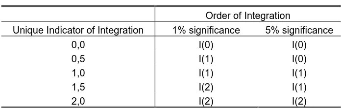
Table 1a presents a synthesis of the existing views with respect to the trend that is characteristic of a series, its relationship with the shocks and its effect on the cycles.

[Table 1 about here]

A stochastic trend implies that each shock is permanent and for that reason is usually called a real shock. In this case, the series present high persistence coefficients.

A deterministic trend, on the other hand, implies that shocks that hit the economy do not deviate it permanently from its long run path. Thus, every shock is transitory.

Assuming a segmented trend implies that the majority of the shocks are transitory and that only one (or a few) is permanent. These are the structural breaks that hit the economy very sporadically. For the case of Argentina, this could be associated with events such as the debt crisis, the convertibility, the Mercosur, the return of democracy or the hyperinflation.

(13)

Clearly, these improvements in the analysis of the data generating process (DGP) should allow for greater precision in the search for the cycle and its features.

I.H. The

methodology

The objective of this paper is to combine a battery of complementary tools to determine the best approximation to the cycle of some of the most relevant macroeconomic time series for Argentina.

Here we present a procedure (that we will follow in the rest of paper) to check for the existence of stationarity or not in the series (and the influence of this fact in the cycle of the variables), as well as for comparing the differences between the cycle assuming a linear trend and a purely stochastic trend (first differences).

Our methodology consists on the following steps:

1. Analyze the first order autocorrelation coefficient of the series (of the cycle of those series) including a recursive and rolling version. The goal is to obtain a first vision of the level of persistence of the series and of the possible changes in the intra-sample behavior.

2. Compare the persistence of the series with respect to that of an artificial series constructed as the average of 2000 Monte Carlo simulations of RW processes. This will allow us to build a Relative Persistence Measure (RPM).

3. Analyze for the hypothesis of Unit Root for the sample as a whole with the Augmented Dickey-Fuller (ADF).

4. Perform the analysis of the hypothesis of Unit Root for the whole sample with the Phillips-Perron (PP) test.

5. Analyze of the hypothesis of Unit Root for the sub-samples with a recursive ADF, obtaining the maximum and minimum.

6. Evaluate the hypothesis of Unit Root for the sub-samples with a rolling ADF, obtaining the maximum and minimum.

7. Perform of the Variance Ratio (VR) for a sequence of k that is sufficiently long.

8. Analyze of the hypothesis of Unit Rood in the presence of structural break: Perron’s test with exogenous selection of the break date.

9. Check the hypothesis of Unit Root in the presence of structural break: Perron’s test with endogenous selection of the break date: additive outliers (AO).

10. Analyze the hypothesis of Unit Root in the presence of structural break: Perron’s test with endogenous selection of the break date: innovation outliers (IO).

11. Evaluate of the information from the tests on the characteristics of the DGP and thus the best specification for the permanent component of the series.

Following this sequence of growing complexity we begin with the eye inspection of the correlograms, then move to the traditional Unit Root tests, double checking with the indicators of persistence and analyzing if there are changes in the order of integration of the series under the hypothesis of structural break and eventually determine when they occurred. We believe that this is an important contribution since as far as we know such an integral analysis does not exist. We’ve found as an immediate antecedent, though partially related to our work, the important paper by Sosa-Escudero (1997). However, the interest there falls exclusively on the GDP. Additionally the series only reaches the year 1992. Another work, also partially related to ours, is that of Ahumada (1992) on cointegration in nominal variables. Sturzenegger (1989) analyzes the kind of shocks affecting Argentina’s GDP using Blanchard and Quah (1989) decomposition. For more recent sources that include most of the convertibility period (which begun in 91:2) Carrera, Féliz and Panigo (1998a, b) present the results for the GDP and inflation in the first paper and on the real exchange rate in the second one10.

10

(14)

I.I. The

data

For this paper we use the data provided by the Argentinean Government’s Statistical Office (INDEC), the Ministry of the Economy and Public Works, the Central Bank and the Economic Commission for Latin America and the Caribbean (ECLAC).

The data was provided by its source in quarterly periodicity (for the period 1980:1 - 1998:4) in every case with the exception of the unemployment rate, the participation rate and employment rate which are of semi-annual periodicity (for the period 1974:1 - 1998:2).

The GDP, Investment and trade balance were provided by the Ministry of the Economy and Publics Works, while wages, CPI, Participation rate, Unemployment rate and Employment rate where provided by the INDEC. We used the passive nominal annual interest rate as the proxy for the interest rate with information provided by ECLAC. Finally, data on M1 and the nominal exchange rate (used to calculate the real exchange rate) were provided by the Central Bank of Argentina (BCRA). The trade balance is presented as a percentage of GDP. The data was transformed by seasonally adjusting it using the X-11 ARIMA methodology, except for the semi-annual variables. We then applied the logarithm function to the series, with the exceptions of the nominal interest rate, the trade balance, M1 growth, inflation and the semi-annual variables which were left untouched because they are all expressed in percentages. We use the software package RATS 4.2.

The real exchange rate was calculated from the nominal exchange rate of the Peso to the American dollar, correcting it by the evolution of Argentina’s and American’s consumer price index (CPI).

We analyze separately M1 and M1 growth, the CPI and inflation (CPI growth) because the log approximation of growth for these series is not applicable due they present strong oscillation in this sample period.

The identification codes of each series are presented in Table 2 in the Appendix at the end of the paper.

II. M

EASURES OF THE PERSISTENCE OF THE MACROECONOMIC

SERIES IN

A

RGENTINA

II.A. The cycle

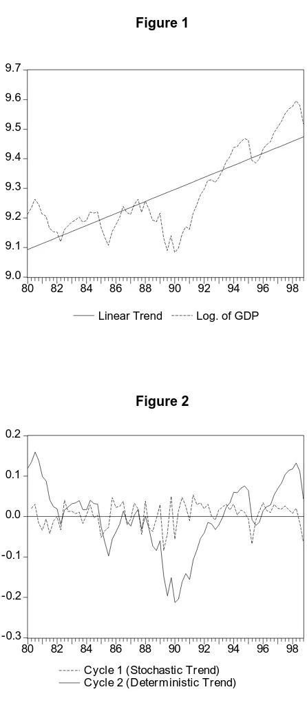
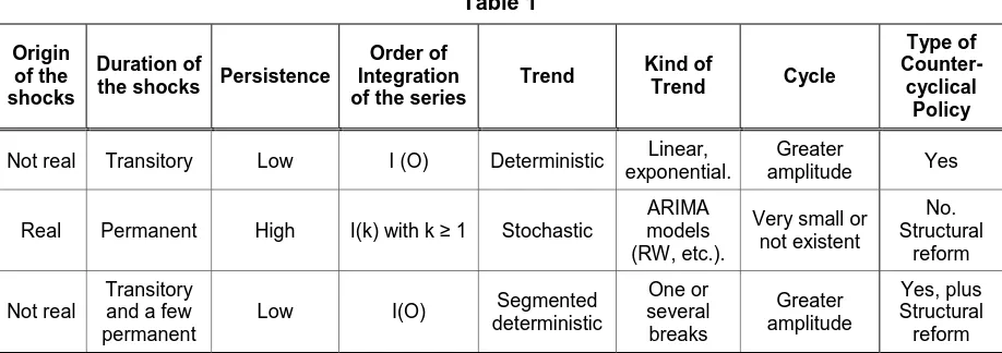
The most traditional (and most often used) way of extracting the cycle relies in a linear deterministic trend such as the one presented in Figure 1. The result is what’s called a deterministic cycle indicated by the thick trace in Figure 2. There we can identify 5 cycles that allow us to interpret the most relevant moments for the macro-economy in Argentina since the 80s.

[Figure 1 and 2 about here]

The first one, ending in 1982, shows the end of the military government. It is dominated mainly by the surge and decadence of the monetarist stabilization plan (which begun in 1978) based on a pre-announced rate of devaluation that resulted to the unsustainable appreciation of the currency (the Peso) and later in a huge financial crisis.

The 1982-85 cycle is the result of the shutting down of the international financial markets after the Mexican default, the change in the political mood with the reinstitution of democratic rule, the statization of the private external debt and several intents of wages and salaries recomposition in the transition to democracy.

(15)

fixation with almost no international reserves. This led the economy to its lowest level in the period in the first quarter of 1990. To grasp the depth of this recession, see, for example, that the GDP at that time was 10% lower in real terms than it was in 1980 (and more than 20% below its long-run deterministic trend).

The fourth cycle starts with a new program based in a floating exchange rate. One of the most drastic credibility measures was taken: to change all of the State’s short term debt and people’s bank deposits, that generated the Central Bank’s huge deficit, into long run debt (nominated in dollars). The program couldn’t avoid a new hyperinflationary shock but it help recover much of the Central Bank’s foreign reserves. This would be key for the move to a new exchange rate fixation where full convertibility of local currency is assumed and the Central Bank’s reserves covered the full monetary base (currency board regime). Known as the Convertibility Plan, this has been the most successful experience as regards a stabilization plan. Together with the effectiveness of the instruments used, the program took advantage of the newly re-opened international financial markets and the important reduction in the international interest rate. In fact, this phase of the cycle with strong growth was interrupted by the recessive crisis resulting from Mexico’s devaluation in 1994 (known as the Tequila effect).

The last cycle identifies with the expansion that begun in 1996, resulting from the reduction in the international interest rate and the fact that the convertibility resisted the previous negative external shock. The new turning point is associated with the international crisis following the crisis in South East Asia.

II.B. What cycle?

When we use a deterministic linear trend such as that in Figure 1, the cycle we obtain is much wider than the one we could get from a stochastic trend. There exist multiple possible stochastic trends. Following the criterion of using the simplest model, we calculated the stochastic cycle as first differences of the logarithm of the series (which for small changes approximate the rates of growth of GDP). In Figure 2 we see the different behavior of the two cycles. In what follows we’ll call Cycle 1 to the one coming from the stochastic trend and Cycle 2 to the other one, resulting from the deterministic trend.

From the comparison, it is evident the different variance in both cycles. Cycle 1 is more homogeneous than Cycle 2 (which shows a behavior with the shape of a V resulting from the deep recession of 1988-89 and the two expansions of the nineties. Defining which kind of cycle is the relevant one has important implications as regards associating economic policies to objectives. Intuitively, we could think that such a point is showing a very strong structural break, especially when from the analysis of the facts it appears as a point of economic change due to the hyperinflationary shock and the change of government. We’ll leave for the end of this paper the formal test for this possibility in an ad-hoc manner as well as endogenously to the data generating process.

The problem that appears with the GDP is common with the rest of the variables so we’ll follow our sequential methodology to try to establish what is the most appropriate DGP for each one.

II.C. Simple measures of persistence

II.C.1. First order correlation coefficients (FOAC)

Following the methodology described in section 1, we obtain the first order autocorrelation coefficients (FOAC), recursive and rolling, for each variable which are presented in figure 3 in the appendix. We find as a common fact that the recursive coefficient in almost all variables grows towards the end of the sample. Amongst the nominal variables such as nominal interest rate (TN), M1 growth (DM) and inflation there’s an abrupt fall in the levels of autocorrelation when we include to the sub-sample the data for the year 1988. In the labor market series it stands out the increasing autocorrelation of the unemployment series.

(16)

For the cycles, the results indicate a highly uniform behavior between the series. Cycle 1 (Stochastic trend) has low autocorrelation, rapidly reverting to its mean, while cycle 2 (Deterministic trend) presents autocorrelation coefficients of around 0.9 for the majority of the series. For the case of the GDP, and complementing what has already been seen in Figure 2, the FOAC of cycle 1 is zero while for cycle 2 is 0.9.

In the nominal variables its important to highlight the structural change that is apparent with the inclusion of the year 1988 (the last stabilization plan of the Radical government) The nominal interest rate, M1 growth and inflation show coefficients that fall to half its value, in cycle 2, or even become negative, in cycle 1 (Stochastic trend).

II.C.2. Relative persistence measure (RPM)

From Table 3 we find patterns of behavior that can be divided into 3 different groups and which are highly stable when we evaluate the series in levels as well as when we evaluate the cycles.

Nominal wages, M1 and the Consumer Price Index (CPI) all show the highest coefficients, them being potentially I (1) and even maybe I (2) series.

In the other extreme, there’s the group of the least persistent series: the nominal interest rate, the growth in M1, inflation and employment. This group even shows negative coefficients for the stochastic trend process. For the stochastic cycle we should also include in the lowest persistence group the real wages, unemployment and the participation rate.

Finally, in the intermediate group we have the GDP, investment, the trade balance and the real exchange rate and, except for the stochastic cycle, the real wages, unemployment and the participation rate.

As we can see from this indicator there is a remarkable stability in the composition of the groups across the different specifications (levels, cycle 1 and cycle 2). However, we should highlight the fact that the value of this indicator (like the FOAC) is strongly affected by the de-trending methodology. For example, the GDP shows values of 0.91, 0.02 and 0.73 for levels, cycle 1 and cycle 2, respectively.

The different de-trending methodologies show strongly contradictory results and for this reason it is necessary to search deeper into the structure of the data generating process (DGP) for each series. In the following section we’ll check for the existence of Unit Root in the autoregressive component of the series using the conventional tests.

II.D. Unit root tests

II.D.1. Augmented Dickey-Fuller (ADF) and Phillips-Perron (PP)

These are the most often used tests in international papers on Unit Root, and thus most useful for international comparisons, even though several criticisms could be expressed about them as we’ve seen in section 1.

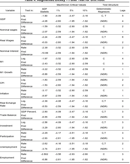
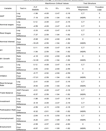
For choosing the number of lags in the ADF test we followed the “General to Specific” methodology. Beginning with 6 lags we established for each series the adequate number of lags for the logarithms of the levels as well as for the first differences of the series. The greatest number of lags was used for the GDP and the real wages and the lowest for the real exchange rate.

For the Phillips-Perron test (PP) we established a uniform number of lags following the Newey-West (1994) criterion that suggests three lags for quarterly series.

With respect the structure of the test as regards what kind of deterministic regressors to use we checked in each case the significativity of using a constant (C), a constant and a trend (C, T) or none of them (NDR). In almost all cases for the first differences we used no deterministic regressors.

The critical values used are those from MacKinnon (1991). The results of the tests are shown in Tables 4 and 5.

With respect to the results of the tests, we found that almost all the series are I (1) under both tests with a conservative hypothesis of 5% significativity.

(17)

One of them is the nominal interest rate for the PP test which results I (0) for any alternative critical value while it appears to be I (1) for the ADF test, also under any critical value. It is interesting to note that this difference appears even though the deterministic regressors are the identical in both cases.

The growth in M1 (dM1) results consistently stationary I (0) in both tests for almost every critical values. Only for the ADF test at 1% the series appears to be I (1). Inflation is another series considered I (0) for both tests at 5%.

M1 (the log level) is an I (2) series for both tests, something which is consistent with the fact that at 1% dM1 was I (1). Only at 10% does M1 appear to be I (1) in the PP test.

The consumer price level (CPI) is another series that shows strong discrepancies between the tests. For the ADF test it is I (2) while for the PP test it is an I (1) series. In the case of the ADF the result is consistent with the fact that inflation is I (1) at 1%, while the result for the CPI with the PP test is consistent with inflation being I (0) in that test. It is probable that the tests are capturing the problems of the hyperinflationary shocks to the economy in different ways.

With respect to I (1) series it is striking the number of them that fall in this category: not only the GDP and investment, but also variables such as the real exchange rate and the trade balance. The indicators from the labor market are also I (1) without exception, from wages (nominal and real) to variables such us the unemployment, employment and the participation rate.

With such strong results we should begin questioning whether this characteristic is caused by the existence of a Unit Root or is just the result of a structural shock that biased the ρ coefficient towards 1. This problem will be looked at more deeply in the following steps of the paper.

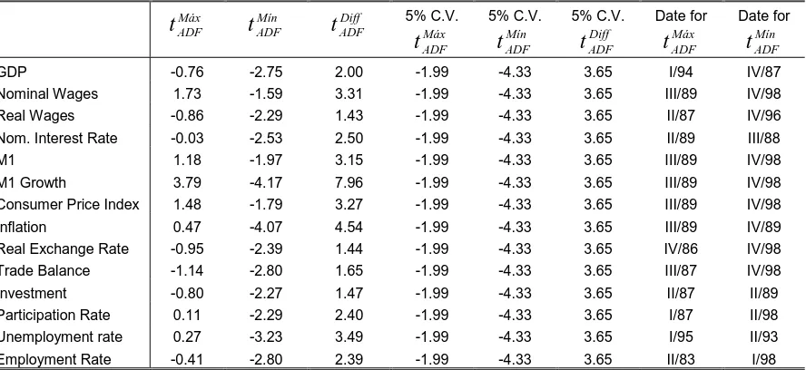
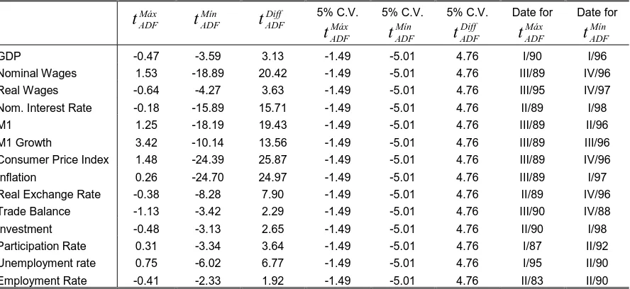
II.D.2. Recursive and Rolling Augmented Dickey-Fuller

Recursive and rolling estimation of ADF t statistics was developed taking k0 = δ0 = 28

observations for quarterly data and k0=δ0 = 20 observations for semiannual data.

The stochastic and deterministic regressors for the rolling and recursive equation are taken from ADF test for the entire sample. The estimated statistics are presented in the Tables 6 to 7 and in the Figure 4 of the appendix. The tabulated 5% critical values are taken form Banerjee et al (1992). In the Figure 4 we present both the Banerjee et al (1992) and the Cheung and Lai (1995) 5% critical values for the minimum ADF t statistic.

We can summarize these results as follows:

The null hypothesis of unit root can not be rejected for any of the variables when recursive methodology and Banerjee’s 5% critical values are used.

If we take the Cheung and Lai’s 5% critical values for the minimum recursive ADF t statistic, M1 growth and inflation become I (0) in the nineties (the only roots that shift with this methodology).

In the rolling estimation the main result is the strong root volatility. For more than 50% of the variables the difference between the maximum and minimum rolling ADF t statistic is bigger than the tabulated critical value. This can be taken as a partial evidence of the existence of structural breaks.

Except for real wages, all prices and monetary variables present a stationary period at the end of the sample (of variable duration11). However this result might be a consequence of the disappearance of the effects of hyperinflation since at the end of the sample, the rolling methodology does not take into account the observations of that period. The question is if the I (0) behavior is the consequence of ouliers from the hyperinflation period or the result of the change of regime with the convertibility.

Finally, there exists strong stability in the results for the National Accounts (GDP, investment and trade balance) and labor market variables (with the exception of nominal wages and unemployment rate). All of them have been I (1) for each sub-sample with the recursive as well as with the rolling estimation methodology.

11

(18)

II.E. Variance ratio test (VR)

While the ADF is a parametric measure of the persistence of the shocks in a series, the one presented by Cochrane (1988) is a non-parametric measure in as much as it does not depend on the selection of the model. In this sense it is a complementary measure to the conventional Unit Root tests.

In Table 8 we present the Variance Ratio Test (VR) for each series in the period 1980-98 following the methodology describe in section 1.

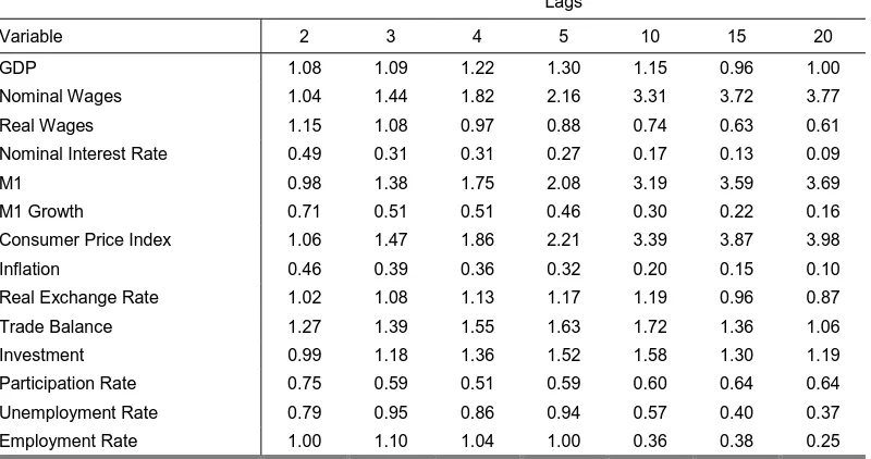
If we take as a reference the VR value after 20 quarters we are able to classify the series in four groups.

The first one includes those variables whose variance grows explosively and have values that tend to 4. Here we find the nominal wages, the CPI and M1. Not only do they show a big number but they also show a trend in that value to grow. This seems to indicate that the series could be I (2) as it was the case for these variables in the previous section (the ADF showed that, at 1% significance, the nominal wages were I (2) too).

Amongst the variables that after 20 quarters still have a persistence of close to 1 we find the GDP (1.0), the real exchange rate (0.87), the trade balance (1.06) and investment (1.16). These series are those best associated with the idea of I (1) series.

The nominal interest rate, growth in M1 and inflation show values of VR!0 when k!∞. This is a strong indication of a stationary series.

The variables of the labor market (with the exception of the nominal wages) conform an independent group with intermediate persistence between 0.25 and 0.64. This could be an indication of the existence of fractional integration (Sowel, 1990) or a structural break.

II.F. Unit root tests under structural break

The possibility that a structural break is the cause why many series that are trend stationary (TSP) appear to be I (1) has been the greatest challenge put forward by Perron to the results accumulated since Nelson and Plosser’s original paper in 1981.

In a great number of papers from this author, his methodology has been consolidating in response to the much of the initial criticism.

Perron’s first test is a conditional test where the date of the structural break is established exogenously by the analyst. One of the most important criticisms resulted from the fact that this produced a pre-testing bias in favor of the non-rejection of the null hypothesis of structural break. The condition of independence in the distribution with respect to the data was not satisfied. For that reason, Perron (1994) and Volgelsang and Perron (1994) developed a testing methodology that allowed for the endogenous detection of the break date. With respect to the use of a priori information, Maddala and Kim (1998) state that this criticisms is partially unjustified since it would not make sense to look for a structural break in the whole sample when we know that there is a significant event. According to the authors, the search should be performed around this event. In this paper, we do exactly that with the change of government in 1989:II and the convertibility in 1991:I.

Following the steps in our methodology from section 1, we’ll analyze the minimum t statistic for ρ=1 in order to detect the structural break in the endogenous alternative, selecting it a priori in the exogenous one.

II.F.1. Perron unit root test with exogenous structural break

In Table 9 we present the results for Perron’s Unit Root test with exogenous structural break for every variable analyzed in this paper. In each one we tested the three alternative models presented in section 1: A) Crash model, that allows for a change in the constant, B) Changing Growth model, that allows for a change in the rate of grow or slope, and model C) that allows for a simultaneous change in both constant and slope.

(19)

For the nominal variables, on the other hand, the most relevant structural change seems to have been dated in the second quarter of 1991 (91:II), with the beginning of the Convertibility Plan (currency board) that, as we’ve already seen, dramatically reduced to international standards the rates of change and the volatility of these variables.

With respect to the real wages we chose as a structural break the third quarter of 1984 (the last “Keynesian” attempt to increase real wages) since from that date on the variable changed its growing trend and begun to fall.

In general terms, the test changed only partially the results of the conventional tests of Unit Root (ADF and PP) or those of the persistence measures (VR).

The GDP, the nominal wages, the trade balance, investment, unemployment and employment are I (1) series even though we allow for the exogenously set structural change.

In the case of the nominal interest rate, in any of the specifications (A, B or C) it appears to be I (0), in contrast with the results for the ADF test and confirming the result of the PP test and the VR that showed a value of 0.09.

In the case of M1, the series appears to be I (1) for every model, contradicting the ADF and PP tests, as well as the VR which showed a value of 3.69. Consistently, dM1 is I (0), confirming the results of the three conventional tests.

In the case of the CPI, the variable is I (1) for every model and this contradicts the ADF and VR results but confirms the PP test.

In the case of the real wages and the real exchange rate if we allow for a break in the slope and in the constant respectively, both show the series to be I (0) at 5%, contradicting the previous results from the ADF and PP tests. However, anticipating this result the VR showed an intermediate value for both series (0.64 and 0.87).

Lastly, the rate of participation turns I (0) when we allow for a change in the slope or in the slope and the constant simultaneously.

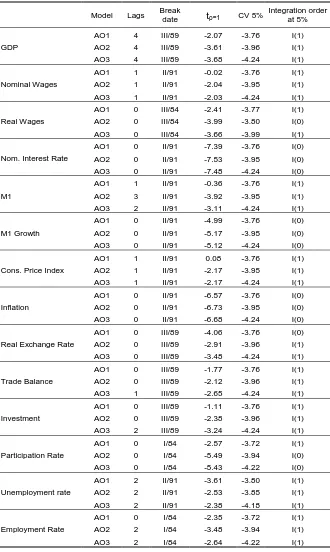
II.F.2. Perron unit root test with endogenous structural break

Of the five possible models, as we’ve seen in section 1, in Table 10 we present the three most relevant, that cover the widest number of results.

The model IO1 allows for a gradual change in the intercept only, the model IO2 allows for the gradual change in the intercept and the slope together and the AO2 allows for a change in the slope.

With respect to an important byproduct such as the date of the structural break, endogenously selected by each model, we observe great dispersion. Model IO2 is the one that most concentrates the breaks around 1988-1989. On the contrary, model IO1 presents the most dispersion in the break dates.

The real wages and the participation rate present the oldest structural breaks, at the beginning of the eighties (approximately 20 quarters before any other variable).

Comparing between models, IO1 model presents 4 variables which are I (0) at 5%, the IO2 model 8 variable I (0) while in the AO2 model only 2 variables appear to be I (0). Only dM1 is considered stationary by all three models. Meanwhile, the nominal interest rate, inflation, unemployment and participation rate are found stationary by at least two models. Undoubtedly, there exists a direct relationship between the number of series that change to being stationary and the flexibility to admit structural changes since IO2 is the model that admits the most shifting coefficients.

As a first result, we highlight the confirmation of the existence of a Unit Root even under the hypothesis of an endogenous structural break (in any of its alternatives) in 5 of the 14 series: the GDP, the real wages, the trade balance, investment and employment.

(20)

With respect to the nominal interest rate, in both IO1 and IO2 models it appears to be a stationary series, coherently with the PP test and VR but in contradiction with the ADF for the complete sample. However, this result is consistent with the rolling ADF that showed stationarity of nominal interest rates in the last period of the sample (the convertibility).

In the labor market, the participation rate is stationary under two alternatives, the same happening with the unemployment rate. This contradicts the ADF and PP results. With respect to the measure of persistence, we observe that both series had intermediate values, especially the participation rate (0.64). These results also contradict those coming from the Rolling ADF where only the unemployment appears stationary during a brief period of time. All other labor market variable are I (1).

III. A

COMPARATIVE ANALISYS

In Table 11 we present a comparative analysis for each variable using every test (eleven) proposed in the methodology.

To build a unique indicator of integration, we took the order of integration suggested by each test for each variable and calculated the average order of integration for every series (Table 2).

[Table 2 about here]

Number 0.5 indicates that the series is I (0) at 5% but I (1) at 1%, a value of 1 states the series is I (1) under both critical values, 1.5 means the series is I (2) at 1% but I (1) at 5%, while a value of 2 indicates the value is I (2) at both 5% and 1%.

In the case of the rolling or recursive ADF tests, a 0.5 value indicates that in an important part of the sample the test shows a change from I (1) for the ADF to I (0) for the complete sample. The analysis of these values should be performed together with the analysis of the dispersion of the results amongst the tests (measured by the variation coefficient) to check for the robustness of the conclusions.

A series with coefficients equal to 1 and small percentage of dispersion in the results can be considered robustly as I (1).

As the coefficients get closer to zero, there is greater possibility that the tests considered the series as I (0).

With values between 0 and 1 we require a detailed analysis of the structure of the results of the different tests. If the rolling ADF and one or several UR tests under the structural break hypothesis signal an I (0) series, then we are in the presence of a variable where the non-stationarity given by the tests for the complete sample (ADF, PP, VR) is an error induced by an extraordinary event. For that reason, the series should be considered stationary. Another possibility is that the series presents fractional integration.

Values higher than 1 are an indication of I (2) series, although we must be cautious with regards to the robustness of this result, since we could find too much dispersion when working with sub-samples due to the possibility of structural breaks.

From the result we can see that the GDP, investment and the trade balance are the only three series that pass all the tests, so we can consider them as robustly I (1). The assumption of a stochastic trend when proceeding to extract the cycle seems to be the best strategy to accurately model the series. In the case of GDP, our results are similar to those of Sosa-Escudero (1997) for the period 1970-92.

The real exchange rate is a non-stationary variable in the sample as a whole. Only for models AO1 and IO2 the variable is considered stationary at 5%. However, with respect to the date of the structural break the majority of the tests indicate that it occurred in the third quarter of 1989 (89:III).