Stand structure and recent climate change constrain stand basal area change in European forests: a comparison across boreal, temperate and Mediterranean biomes

Texto completo

(1)BIBLIOTECA. Document downloaded from the institutional repository of the University of Alcala: http://dspace.uah.es/dspace/. This is a postprint version of the following published document: Ruiz-Benito, P. et al., 2014. Stand Structure and Recent Climate Change Constrain Stand Basal Area Change in European Forests: A Comparison Across Boreal, Temperate, and Mediterranean Biomes. Ecosystems, 17(8), pp.1439–1454. Available at http://dx.doi.org/10.1007/s10021-014-9806-0 © 2014 Springer Verlag. (Article begins on next page). This work is licensed under a Creative Commons Attribution-NonCommercial-NoDerivatives 4.0 International License..

(2) See discussions, stats, and author profiles for this publication at: https://www.researchgate.net/publication/265473376. Stand Structure and Recent Climate Change Constrain Stand Basal Area Change in European Forests: A Comparison Across Boreal, Temperate, and Mediterranean Biomes Article in Ecosystems · August 2014 DOI: 10.1007/s10021-014-9806-0. CITATIONS. READS. 24. 252. 8 authors, including: Paloma Ruiz-Benito. Jaime Madrigal-González. University of Acalá. Institute for Environmental Sciences, University of Geneva. 72 PUBLICATIONS 1,054 CITATIONS. 52 PUBLICATIONS 369 CITATIONS. SEE PROFILE. SEE PROFILE. Sophia Ratcliffe. David Coomes. National Bioversity Network Trust. University of Cambridge. 34 PUBLICATIONS 488 CITATIONS. 267 PUBLICATIONS 13,668 CITATIONS. SEE PROFILE. SEE PROFILE. Some of the authors of this publication are also working on these related projects:. The role of tree species composition and forest structure on cooling as forest ecosystem service provision View project. PN-II-ID-PCE-2011-3-0781 Forest GHG Management View project. All content following this page was uploaded by Paloma Ruiz-Benito on 25 January 2015.. The user has requested enhancement of the downloaded file..

(3) Ecosystems. Stand structure and recent climate change constrain stand basal area change in European forests: a comparison across boreal, temperate and Mediterranean biomes. r Fo Journal:. Manuscript ID: Types:. Date Submitted by the Author:. ECO-13-0326.R3 Original Article n/a. Pe. Complete List of Authors:. Ecosystems. er. Ruiz-Benito, Paloma; University of Stirling, Biological and Environmental Sciences; University of Alcala, Forest Ecology and Restoration Group, Department of Life Sciences; Forest Research Center - Instituto Nacional de Investigación y Tecnología Agraria y Alimentaria (CIFOR-INIA, Department of Forest Ecology and Genetics Madrigal-Gonzalez, Jaime; University of Alcala, Forest Ecology and Restoration Group, Department of Life Sciences Ratcliffe, Sophie; University of Leipzig, AG Spezielle Botanik und Funktionelle Biodiversität Coomes, David; University of Cambridge, Plant Sciences Kaendler, Gerald; The Forest Research Institute, Lehtonen, Aleksi; Metla, Carbon Wirth, Christian; University of Leipzig, AG Spezielle Botanik und Funktionelle Biodiversität; German Centre for Integrative Biodiversity Research (iDiv), Zavala, Miguel; University of Alcala, Forest Ecology and Restoration Group, Department of Life Sciences. ew. vi. Re. Key Words:. carbon sink, climatic variability, competition, inventory-based data, minimum temperature, mixed models, stand basal area change, water availability.

(4) Page 1 of 56. Ruiz-Benito et al. 1 1. Stand structure and recent climate change constrain stand basal area change in. 2. European forests: a comparison across boreal, temperate and Mediterranean. 3. biomes. 4. Short title: Drivers of basal area change across Europe. 5. P. Ruiz-Benito1,2,3*, J. Madrigal-González2 (ecojmg@hotmail.com), S. Ratcliffe4. 6. (sophia.ratcliffe@uni-leipzig.de), D. A. Coomes5 (dac18@cam.ac.uk), G. Kändler6. 7. (Gerald.Kaendler@forst.bwl.de), A. Lehtonen7 (aleksi.lehtonen@metla.fi), C. Wirth4,8. 8. (cwirth@uni-leipzig.de), M. A. Zavala2 (madezavala@gmail.com),. rP. Fo. 9 10 11. 1. 12 13. 2. 14 15. 3. 16 17. 4. 18 19. 5. 20. 6. 21 22. 7. 23 24. 8. 25. Correspondence: Paloma Ruiz Benito. E-mail: palomaruizbenito@gmail.es. Phone: 00 34 637. 26. 19 43 53. Fax: 00 34 91 357 22 93.. 27. Type of paper: Original Article. Department of Forest Ecology and Genetics, ForestResearch Center - Instituto Nacional de Investigación y Tecnología Agraria y Alimentaria (CIFOR-INIA), Ctra. de la Coruña, Km. 7,5. 28040. Madrid, Spain.. ee. Forest Ecology and Restoration Group, Department of Life Sciences, Science Building, University of Alcala, Campus Universitario, 28871, Alcalá de Henares (Madrid), Spain.. rR. Biological and Environmental Sciences, School of Natural Sciences.University of Stirling. FK9 4LA, Stirling, United Kingdom.. ev. University of Leipzig. AG Spezielle Botanik und Funktionelle Biodiversität. Johannisallee 21-2. 04103 Leipzig, Germany.. iew. 1 2 3 4 5 6 7 8 9 10 11 12 13 14 15 16 17 18 19 20 21 22 23 24 25 26 27 28 29 30 31 32 33 34 35 36 37 38 39 40 41 42 43 44 45 46 47 48 49 50 51 52 53 54 55 56 57 58 59 60. Ecosystems. Forest Ecology and Conservation Group, Department of Plant Sciences, University of Cambridge, Downing Street, Cambridge, CB3 2EA, UK. The Forest Research Institute, Wonnhaldestr. 4. 79100 Freiburg, Germany.. Finnish Forest Research Institute, Vantaa Research Centre, PO Box 18, 01301 Vantaa, Finland. German Centre for Integrative Biodiversity Research (iDiv) Halle-Jena-Leipzig, Deutscher Platz 5e, 04103 Leipzig, Germany..

(5) Ecosystems. Ruiz-Benito et al. 2 28. Authorship: JM, PRB and MAZ conceived the design; DC, GK, AL, SR, PRB, CW and MAZ. 29. collected the data; JM, PRB and SR analyzed data; DC, JM, SR and PRB contributed to the. 30. methods, and all the authors wrote the article.. 31. iew. ev. rR. ee. rP. Fo. 1 2 3 4 5 6 7 8 9 10 11 12 13 14 15 16 17 18 19 20 21 22 23 24 25 26 27 28 29 30 31 32 33 34 35 36 37 38 39 40 41 42 43 44 45 46 47 48 49 50 51 52 53 54 55 56 57 58 59 60. Page 2 of 56.

(6) Page 3 of 56. Ruiz-Benito et al. 3 32. ABSTRACT. 33. European forests have a prominent role in the global carbon cycle and an increase in. 34. carbon storage has been consistently reported during the 20th century. Any further. 35. increase in forest carbon storage, however, could be hampered by increases in aridity. 36. and extreme climatic events. Here we use forest inventory data to identify the relative. 37. importance of stand structure (stand basal area and mean d.b.h.), mean climate (water. 38. availability) and recent climate change (temperature and precipitation anomalies) on. 39. forest basal area change during the late 20th century in three major European biomes.. 40. Using linear mixed-effects models we observed that stand structure, mean climate and. 41. recent climatic change strongly interact to modulate basal area change. Although we. 42. observed a net increment in stand basal area during the late 20th century, we found the. 43. highest basal area increments in forests with medium stand basal areas and small to. 44. medium sized trees. Stand basal area increases correlated positively with water. 45. availability, and were enhanced in warmer areas. Recent climatic warming caused an. 46. increase in stand basal area, but this increase was offset by water availability. Based on. 47. recent trends in basal area change we conclude that the potential rate of aboveground. 48. carbon accumulation in European forests strongly depends on both stand structure and. 49. concomitant climate warming, adding weight to suggestions that European carbon. 50. stocks may saturate in the near future.. 51. Keywords: carbon sink, climatic variability, competition, inventory-based data,. 52. minimum temperature, mixed models, water availability, stand basal area change.. iew. ev. rR. ee. rP. Fo. 1 2 3 4 5 6 7 8 9 10 11 12 13 14 15 16 17 18 19 20 21 22 23 24 25 26 27 28 29 30 31 32 33 34 35 36 37 38 39 40 41 42 43 44 45 46 47 48 49 50 51 52 53 54 55 56 57 58 59 60. Ecosystems.

(7) Ecosystems. Ruiz-Benito et al. 4 53. INTRODUCTION. 54. Forests cover more than 30% of the global land surfaces (FRA, 2010), store large. 55. reservoirs of carbon (Goodale and others 2002; Pan and others 2011), harbour around. 56. two thirds of terrestrial biodiversity (Millennium Ecosystem Assessment 2005) and. 57. promote multiple ecosystem services (Gamfeldt and others 2013). Forests play a central. 58. role in the global carbon cycle, but the factors controlling terrestrial carbon exchanges. 59. and their magnitude remain controversial (Valentini and others 2000; Nabuurs and. 60. others 2003; Bellassen and Luyssaert 2014). For example, it is widely accepted that. 61. current increases in forest biomass observed in many temperate forests result partially. 62. from positive effects of global change (e.g. Pastor and Post 1988; Nabuurs and others. 63. 2003; Ciais and others 2008; Hember and others 2012; Peng and others 2014) and. 64. changes in forest management regimes (e.g. Spiecker 1999; Luyssaert and others 2010),. 65. but the influences of climate change and extreme climatic events on biomass changes. 66. are not well understood (Dixon and others 1994; Schimel 2007; McMahon and others. 67. 2010).. ev. rR. ee. rP. Fo. 68. Future forest carbon sinks could be affected by large-scale changes in mortality. 69. and growth rates, both of which are related to climate, forest structure and the. 70. interactions between these factors (e.g. van Mantgem and others 2009; Dietze and. 71. Moorcroft 2011; Ruiz-Benito and others 2013). The rate of increase in carbon storage. 72. depends on forest structure, climate warming, CO2 fertilisation and nitrogen deposition. 73. effects (Nabuurs and others 2003; Ciais and others 2008; Pan and others 2011).. 74. Although the magnitude of these effects remains uncertain, it has been shown that. 75. recent climate change and CO2 fertilisation could have a positive impact on tree growth. 76. (Cao and Woodward 1998; Ciais and others 2008; Bellassen and others 2011).. 77. However, these positive effects could be overwhelmed by the effects of increased. iew. 1 2 3 4 5 6 7 8 9 10 11 12 13 14 15 16 17 18 19 20 21 22 23 24 25 26 27 28 29 30 31 32 33 34 35 36 37 38 39 40 41 42 43 44 45 46 47 48 49 50 51 52 53 54 55 56 57 58 59 60. Page 4 of 56.

(8) Page 5 of 56. Ruiz-Benito et al. 5 78. climatic variability and extreme climatic events, such as more frequent and more intense. 79. drought events (e.g. Ciais and others 2005; Zhao and Running 2010; Hoch and Körner. 80. 2012). Moreover, regional studies have not shown consistent trends in forest growth. 81. rates; growth is increasing in temperate areas but no clear trends have been found in. 82. European boreal or Mediterranean forests (Spiecker, 1999). On the other hand, recent. 83. worldwide episodes of increased defoliation and tree mortality have been related to. 84. climate-induced processes (Allen and others 2010; Carnicer and others 2011). Forest. 85. carbon sinks could be potentially affected by large-scale changes in mortality and. 86. growth rates, both of which have been related to climate and/or its interaction with. 87. forest structure (e.g. van Mantgem and others 2009; Dietze and Moorcroft 2011; Ruiz-. 88. Benito and others 2013).. ee. rP. Fo. 89. European forests have been globally important carbon sinks (Ciais and others. 90. 2008; Nabuurs and others 2003), but what will happen in future is a matter of intense. 91. debate (Narbuurs and others 2013). As a result of climate change, mean temperatures. 92. are likely to increase, with northern Europe experiencing warmer winters and. 93. Mediterranean regions warmer summers (Christensen and others 2007). Meanwhile,. 94. climate change scenarios suggest that precipitation could increase in northern Europe. 95. and decrease in Mediterranean regions (Christensen and others 2007). The exposure of. 96. Mediterranean systems to even hotter, drier summers could result in the death of trees. 97. normally regarded as drought tolerant, because the combination of low soil moisture. 98. potentials and strong vapour pressure deficits push water transport systems to their limit. 99. (Allen and others 2010; Ruiz-Benito and others 2013). Thus, climate change could. 100. result in a reduction of carbon gains in the water-limited forests of Europe (Vayreda and. 101. others 2012), that could even counteract gains arising from the abandonment of. 102. agricultural lands (Canadell and Raupach 2008).. iew. ev. rR. 1 2 3 4 5 6 7 8 9 10 11 12 13 14 15 16 17 18 19 20 21 22 23 24 25 26 27 28 29 30 31 32 33 34 35 36 37 38 39 40 41 42 43 44 45 46 47 48 49 50 51 52 53 54 55 56 57 58 59 60. Ecosystems.

(9) Ecosystems. Ruiz-Benito et al. 6 103. Understanding how forest structure and climate interact to drive biomass change. 104. across European forests, from boreal to temperate and Mediterranean forests is critical. 105. to infer future trends in forest carbon sinks. The role of European forests in the global. 106. carbon cycle in the second half of the 20th century has been largely estimated through. 107. inventory-based national statistics (e.g. Goodale and others 2002; Nabuurs and others. 108. 2003; Ciais and others 2008; Bellassen and others 2011). Recently tree level. 109. information from consecutive inventories has become available in a growing number of. 110. EU countries, allowing us to better estimate large-scale demographic processes (e.g.. 111. Kunstler and others 2011; Benito-Garzón and others 2013; García-Valdés and others. 112. 2013, Vilà and others 2013). In this study we performed, for the first time, a large-scale. 113. analysis of the main patterns and drivers of recent stand basal area change in the three. 114. main biomes of European forests, using plot-level forest inventory information. Our. 115. specific objectives were: (i) to examine recent decadal patterns of forest basal area. 116. change, growth and mortality across Mediterranean, temperate and boreal biomes in. 117. Europe; and (ii) to quantify the effect of stand structure, mean climate and recent. 118. climate change on stand basal area change.. 119. MATERIAL AND METHODS. 120. Data of stand basal area change and its components. 121. We compiled information from consecutive National Forest Inventories (NFI hereafter). 122. of Spain, Germany and Finland (see methodological details in Appendix 1 of. 123. supplementary material), which encompass stands belonging to Mediterranean,. 124. temperate and boreal biomes (Figure 1a). We selected plots from consecutive surveys. 125. where tree-level data on ingrowth, surviving and dead trees was recorded in both. 126. surveys (see supplementary Appendix 1 and Table S1).. iew. ev. rR. ee. rP. Fo. 1 2 3 4 5 6 7 8 9 10 11 12 13 14 15 16 17 18 19 20 21 22 23 24 25 26 27 28 29 30 31 32 33 34 35 36 37 38 39 40 41 42 43 44 45 46 47 48 49 50 51 52 53 54 55 56 57 58 59 60. Page 6 of 56.

(10) Page 7 of 56. Ruiz-Benito et al. 7 127. From the initial plots of the three NFIs we selected a total of 40,521 plots where. 128. at least one adult tree was measured (i.e. d.b.h. > 10 cm) and where there was no. 129. evidence of thinning or harvesting in either of the two consecutive surveys. Plots with. 130. any sign of harvesting were excluded for two reasons: (i) biomass loss due to harvesting. 131. implies an assessment of growth considering only surviving trees, which could result in. 132. biased estimates of real productivity in natural forests ; and (ii) harvesting usually. 133. triggers an immediate growth release in neighbouring trees and, therefore, management. 134. could affect carbon stock changes (Vayreda and others 2012).. Fo. 135. In the 40,521 plots each tree alive in the first inventory was recorded as either. 136. alive or dead in the second inventory. We estimated the absolute change in basal area. 137. and the relative growth and mortality rates in each plot. Thus, we calculated: (i) stand. 138. basal area change (m2 ha-1 yr-1, SBAc hereafter) as the difference in stand basal area. 139. between the two surveys with respect to the time interval; (ii) basal area growth rate. 140. (annual percentage, SBAgain) as the sum of basal area increments of all live trees present. 141. in each survey with respect to the time interval and initial stand basal area; and (iii). 142. basal area loss rate due to natural mortality (annual percentage, SBAloss) as the basal. 143. area lost between consecutive surveys due to mortality, again with respect to the initial. 144. stand basal area and time interval following Sheil and others (1995). Basal area loss rate. 145. was greater than zero in 25.4% of the plots included in this analysis (i.e. from the. 146. 40,521 measured plots included in this analysis 10,303 had a basal area loss rate greater. 147. than zero). We used stand basal area change instead of biomass change directly because:. 148. (i) basal area has been identified as reliable a proxy for biomass (e.g. Slik and others. 149. 2010); (ii) allometric equations do not exist for all 158 species present in the 40,521. 150. plots included in the analysis; and (iii) allometric relationships can vary along the large. 151. climatic gradient covered in this study (e.g. Lines and others 2012). We produced maps. iew. ev. rR. ee. rP. 1 2 3 4 5 6 7 8 9 10 11 12 13 14 15 16 17 18 19 20 21 22 23 24 25 26 27 28 29 30 31 32 33 34 35 36 37 38 39 40 41 42 43 44 45 46 47 48 49 50 51 52 53 54 55 56 57 58 59 60. Ecosystems.

(11) Ecosystems. Ruiz-Benito et al. 8 152. of SBAc, SBAgain and SBAloss using ArcGIS 10 (ESRI Inc., Redlands, CA, USA; Figure. 153. 1).. 154. Forest structure and climate data. 155. We used two forest structure variables, two climatic variables and two variables. 156. representative of recent climatic change as potential predictors of recent stand basal area. 157. changes. Mean tree diameter (dm, mm) and stand basal area (BA, m2 ha-1), in the first. 158. survey, were used to represent forest structure.. Fo. 159. To characterise the spatial variability of climate across the three biomes, for each. 160. of the plots we obtained climatic variables from WorldClim (Hijmansand others 2005). 161. and CGIAR-CSI GeoPortal, using CGIAR-CSI Global-Aridity and Global-PET. 162. Database (Zomer and others 2007; 2008). Two climatic variables were selected to. 163. characterise the climate in each plot (see details of variable selection in supplementary. 164. Appendix 2 and Table S2): an index of water availability (WAI) and mean temperature. 165. of the coldest quarter (hereafter minimum temperature, Tmin) (based on data between. 166. 1950 and 2000). WAI integrates temperature and rainfall in each plot (i.e. annual. 167. precipitation. 168. evapotranspiration). Negative values of WAI correspond to dry areas and positive. 169. values to wet areas, and it has been shown to be an important driver of tree carbon. 170. storage in the Mediterranean region (Vayreda and others 2012). Minimum temperature. 171. is thought to be an important constraint in eastern European limits of tree species. 172. distribution (e.g. Sykes and Prentice 1996).. minus. potential. iew. ev. rR. ee. rP. 1 2 3 4 5 6 7 8 9 10 11 12 13 14 15 16 17 18 19 20 21 22 23 24 25 26 27 28 29 30 31 32 33 34 35 36 37 38 39 40 41 42 43 44 45 46 47 48 49 50 51 52 53 54 55 56 57 58 59 60. Page 8 of 56. evapotranspiration. divided. by. potential. 173. The magnitude of recent climate change was quantified by comparing mean. 174. annual temperature and precipitation over the study period with the mean of each. 175. climatic variable over the reference period 1900-2006, using mean monthly climate data.

(12) Page 9 of 56. Ruiz-Benito et al. 9 176. at 0.5 x 0.5 degree resolution from UDel_AirT_Precip data provided by the. 177. NOAA/OAR/ESRL PSD (Boulder, Colorado, USA). The study period was defined as. 178. the number of years between the two consecutive inventories plus two years before the. 179. first survey (i.e. 1984-2006 Spain; 1984-2002 Germany; 1983-1995 Finland) to include. 180. lagged effects of climate on growth or mortality (Vayreda and others 2012). We. 181. calculated absolute temperature anomalies and relative precipitation anomalies, using. 182. yearly averages calculated using mean monthly climate data (i.e. from January to. 183. December). The absolute temperature anomaly (ºC) was defined as the difference. 184. between the mean temperature for the study period and the mean value for the reference. 185. period (1900-2006). The relative precipitation anomaly (%) was defined as the ratio. 186. between the equivalent differences for precipitation and the mean value for precipitation. 187. for the reference period. The absolute temperature anomalies varied from -0.3 to 1 ºC. 188. among grid cells (with an average increment of 0.46 ºC), while the relative precipitation. 189. anomalies varied from -18.7% to 14.6% (with an average of -2.5%, see supplementary. 190. Figure S1 and S2).. 191. Statistical analyses. iew. ev. rR. ee. rP. Fo. 1 2 3 4 5 6 7 8 9 10 11 12 13 14 15 16 17 18 19 20 21 22 23 24 25 26 27 28 29 30 31 32 33 34 35 36 37 38 39 40 41 42 43 44 45 46 47 48 49 50 51 52 53 54 55 56 57 58 59 60. Ecosystems. 192. We modelled stand basal area change (SBAc, m2 ha-1 yr-1) using linear mixed-. 193. effects models, with a Gaussian distribution of residuals and used an identity link for the. 194. response variable. All analyses were performed in R version 2.15.1 (R Core Team. 195. 2012), using the “lme4” package (Bates and others 2012).. 196. The six fixed predictor variables of SBAc used were: stand basal area (BA,. 197. m2/ha), mean d.b.h. (dm, mm), water availability (WAI, %), minimum temperature. 198. (Tmin, ºC), absolute temperature anomaly (TA, ºC) and relative precipitation anomaly. 199. (PA, %) (see mean values in supplementary Figure S3 and Table S3). Due to the.

(13) Ecosystems. Ruiz-Benito et al. 10 200. clustered nature of the sampling in Finland and Germany (where plots are aggregated in. 201. groups of four; see Appendix 1 for more information), we included cluster as a random. 202. effect in the model. We fitted country as a fixed effect because it only has three levels,. 203. and as such is inappropriate as a random effect (see Bolker and others 2009). Our full. 204. model also included as fixed effects linear and quadratic terms for each explanatory. 205. variable. Based on our initial hypothesis we also included pair-wise interactions. 206. between stand structure and climate variables: dm × BA, WAI × Tmin, BA × WAI, BA ×. 207. Tmin, BA × TT, BA × PT, dm × WAI, dm × Tmin, dm × TT, dm × PT and WAI × TT, WAI. 208. ×. 209. mean was subtracted from each value and divided by the standard deviation), enabling. 210. the interactions to be included in the model (Zuur and others 2009). Additionally, in. 211. order to detect colinearity between explanatory variables, we calculated the variance. 212. inflation factors (VIFs) for each predictor variable. VIFs calculate the degree to which. 213. collinearity inflates the estimated regression coefficients as compared with the. 214. orthogonal predictors (Belsey, 1991; Oksanen and others 2010). Our results confirmed. 215. that collinearity was not a major problem in our data (VIF < 3).. Fo. PT and Tmin × TT. All the numerical predictor variables were standardised (i.e. the. iew. ev. rR. ee. rP. 1 2 3 4 5 6 7 8 9 10 11 12 13 14 15 16 17 18 19 20 21 22 23 24 25 26 27 28 29 30 31 32 33 34 35 36 37 38 39 40 41 42 43 44 45 46 47 48 49 50 51 52 53 54 55 56 57 58 59 60. Page 10 of 56. 216. The most parsimonious model was determined using BIC (Bayesian Information. 217. Criterion) as an indicator of both parsimony and likelihood (Burnham and Anderson. 218. 2002). To identify the best-supported model we first constructed candidate models in. 219. which each of the interactions were dropped and if the difference in BIC between the. 220. reduced and full models was less than two then the simpler model was selected (Hilborn. 221. and Mangel 1997; Pinheiro and Bates 2000). The process was then repeated for all the. 222. independent variables this time comparing each individual predictor variable with a. 223. model containing all response variables without any interactions, using the differences. 224. in BIC to quantify the relative importance of each predictor variable. Finally, parameter.

(14) Page 11 of 56. Ruiz-Benito et al. 11 225. estimates and confidence intervals of the best-supported model were obtained using. 226. restricted maximum likelihood (REML), which minimizes the likelihood of the. 227. residuals from the fixed-effect portions of the model (Zuur and others 2009).. 228. The marginal R2 (proportion of variance explained by fixed factors) and. 229. conditional R2 (proportion of variance explained by both the fixed and random factors). 230. were estimated following Nakagawa and Schielzeth (2013). The parameter estimates. 231. provide the basis for determining the magnitude of the effect of a given process, with. 232. maximum likelihood estimates of parameter values close to zero indicating no effect.. 233. Mean parameter estimates and 95% confidence intervals for the fixed effects were. 234. estimated using bootstrapping methods available in the lme4 package (Bates and others. 235. 2012).. ee. rP. Fo. 236. Response curves for each explanatory variable (varying between the 99%. 237. percentiles observed in the data) were computed using the best supported model, fixing. 238. the values of the other continuous variables at the observed mean (Table 1), and the. 239. categorical variables to zero (i.e. the fixed country effect, Eq. (1)). Approximate. 240. confidence intervals of the prediction were calculated from the variance-covariance. 241. matrix of the fixed effects (± 2 × standard error of prediction). Response curves were. 242. also computed with two variables varying between the 99% percentiles observed in the. 243. data, with the rest held constant to the mean; these were visualised using three-. 244. dimensional graphs.. iew. ev. rR. 1 2 3 4 5 6 7 8 9 10 11 12 13 14 15 16 17 18 19 20 21 22 23 24 25 26 27 28 29 30 31 32 33 34 35 36 37 38 39 40 41 42 43 44 45 46 47 48 49 50 51 52 53 54 55 56 57 58 59 60. Ecosystems.

(15) Ecosystems. Ruiz-Benito et al. 12. 245. RESULTS. 246. Patterns of stand basal area change and its components. 247. During the late 20th century there were positive mean stand basal area changes (SBAc). 248. in the Mediterranean, temperate and boreal biomes (Table 1, supplementary Table S3),. 249. confirming that forests in these regions were accumulating basal area at a mean relative. 250. annual rate of 3.82%. We observed the largest mean SBAc, growth and loss rates in the. 251. temperate biome (Table 1, Figure 1b-d), with the highest basal area loss rates occurring. 252. in Spanish temperate forests (i.e. Northern Iberian Peninsula, see Figure 1d and. 253. supplementary Table S3). Forests with negative or near-zero SBAc were mainly. 254. concentrated in the Mediterranean and northern boreal regions (Table 1, Figure 1b).. 255. There was a positive correlation between SBAc and relative basal area gains due to. 256. growth (r = 0.41, P < 0.001, Figure 1b,c), but SBAc was also affected by natural. 257. mortality as it can be observed by the negative correlation between SBAc and basal area. 258. loss (r = -0.26, P < 0.001, Figure 1b,d).. ev. rR. ee. rP. Fo. 259. A latitudinal gradient in water availability (WAI) and minimum temperature was. 260. observed (supplementary Figure S1). The Mediterranean biome had the driest areas (i.e.. 261. negative WAI) with increasing water availability towards the temperate and boreal. 262. biomes (Table 1), and minimum temperatures were lowest in the boreal biomes (Table. 263. 1). Regarding climatic anomalies in the late 20th century, the largest temperature. 264. increments and precipitation reductions tended to be concentrated in Mediterranean and. 265. cool temperate biomes (Table 1 and supplementary Figure S1).. 266. Effects of stand structure, climate and recent climate change on basal. 267. area change. iew. 1 2 3 4 5 6 7 8 9 10 11 12 13 14 15 16 17 18 19 20 21 22 23 24 25 26 27 28 29 30 31 32 33 34 35 36 37 38 39 40 41 42 43 44 45 46 47 48 49 50 51 52 53 54 55 56 57 58 59 60. Page 12 of 56.

(16) Page 13 of 56. Ruiz-Benito et al. 13 268. The best-supported model included the effects of all predictor variables (marginal R2 =. 269. 0.2743, conditional R2 = 0.3761) and took the following functional form:. 270 271 272 273 274 275. (1). Fo. 276. rP. 277. where the response variable is the absolute stand basal area change (SBAc), and the. 278. numerical predictor variables were: stand basal area (BA), mean d.b.h. (dm), minimum. 279. temperatures (Tmin) and precipitation anomalies (PA) as quadratic terms; and water. 280. availability (WAI) and temperature anomalies (TA) as linear terms (see Table 2 and. 281. supplementary Table S4 for model comparisons, Table 3 for fitted parameter values,. 282. supplementary Figure S4 for observed and predicted SBAc and supplementary Figure. 283. S5 for model residuals). Country (i.e. Spain, Germany and Finland) was included as a. 284. fixed categorical effect and thus linear terms were also included for Spain (SP) and. 285. Finland (FI).. iew. ev. rR. ee. 1 2 3 4 5 6 7 8 9 10 11 12 13 14 15 16 17 18 19 20 21 22 23 24 25 26 27 28 29 30 31 32 33 34 35 36 37 38 39 40 41 42 43 44 45 46 47 48 49 50 51 52 53 54 55 56 57 58 59 60. Ecosystems. 286. BIC model comparisons indicated that mean d.b.h. had the largest effect on. 287. SBAc, followed by WAI, stand basal area, temperature anomaly and minimum. 288. temperature (Table 2). The relative precipitation anomaly explained the smallest. 289. variation compared to the rest of explanatory variables (Table 2). With regards to the. 290. interaction terms, it is important to note that the full model included all possible pair-. 291. wise interactions between the stand structure and climatic variables, but also strong. 292. interactions between climate and recent climatic anomalies were found (Table 2,3)..

(17) Ecosystems. Ruiz-Benito et al. 14 293. The largest SBAc was observed in stands dominated by small trees (dm< 200. 294. mm). SBAc decreased rapidly with mean tree diameter up to c. 9800 mm after which it. 295. increased again (Figure 2). Considering stand basal area, SBAc increased from low to. 296. medium stand basal area values, stabilising from medium to high stand basal area. 297. values (Figure 2).. 298. The effect of WAI on SBAc was particularly strong in stands with low mean. 299. d.b.h. (Figure 3a) and low basal area (Figure 3b). With increasing minimum. 300. temperature, a non-linear relationship with SBAc was observed with a SBAc peak at. 301. intermediate temperatures (Figure 4c), but this relationship was strongly affected by. 302. mean d.b.h. (Figure 3c) and stand basal area (Figure 3d). The positive effect of. 303. increasing minimum temperature on SBAc was particularly strong at high mean d.b.h.,. 304. showing a more neutral relationship at low mean d.b.h. (Figure 3c). Stands with low. 305. basal area showed the lowest SBAc at negative minimum temperatures, and the highest. 306. SBAc at high basal area (Figure 3d). Moreover, we observed that the effect of minimum. 307. temperature on SBAc was greater in wet areas (WAI positive) than in dry areas (WAI. 308. negative) (Figure 4a). SBAc was positively associated with water availability (i.e. WAI). 309. in hot regions (i.e. Figure 4a,b) but no such relationship was found in regions with low. 310. minimum temperatures (Figure 4a).. iew. ev. rR. ee. rP. 311. Fo. 1 2 3 4 5 6 7 8 9 10 11 12 13 14 15 16 17 18 19 20 21 22 23 24 25 26 27 28 29 30 31 32 33 34 35 36 37 38 39 40 41 42 43 44 45 46 47 48 49 50 51 52 53 54 55 56 57 58 59 60. Page 14 of 56. We observed an increase in SBAc with increases in recent temperature. 312. anomalies (see positive value of parameter. 313. warming on SBAc was particularly strong in stands with low mean d.b.h. (Figure 3e). 314. and high basal area (Figure 3f). The positive effect of recent temperature increase on. 315. SBAc was also particularly high in wet areas, turning to neutral in dry sites (Figure 4b).. 316. The positive effect of recent temperature increase was observed along the full length of. 317. the minimum temperature gradient and was particularly strong at low minimum. , Table 3). This positive effect of recent.

(18) Page 15 of 56. Ruiz-Benito et al. 15 318. temperatures (Figure 4c). The negative effects of recent precipitation reductions on. 319. SBAc increments were observed in both dry and wet areas, but the positive effects of. 320. precipitation increase only occurred in wet areas (i.e. positive WAI, Figure 4d).. 321. DISCUSSION. 322. The plot-based forest inventory information from Spain, Germany and Finland showed. 323. that in the late 20th century undisturbed European forests experienced a net increase in. 324. stand basal area, in agreement with previous studies (e.g. Ciais and others 2008;. 325. Bellassen and others 2011). These increments were particularly large in the temperate. 326. biome, turning to neutral or even negative in some areas of the Mediterranean and. 327. northern boreal forests. Patterns of stand basal area increase were highly influenced by. 328. stand structure (mean d.b.h. and stand basal area) and climate (water availability and. 329. minimum temperatures), but also by recent temperature and precipitation anomalies.. 330. The largest stand basal area changes (SBAc) occurred in relatively young forests or. 331. forests in early development stages (i.e. low mean d.b.h. and low-medium basal area) in. 332. mesic environments (i.e. not constrained by water or energy availability). Together,. 333. these results suggest that the carbon sink potential of European forests could be strongly. 334. constrained in water-limited Mediterranean forests, where the positive effects of recent. 335. climate warming may be offset by competition and climatic stress.. 336. Patterns of stand basal area change and its components. 337. All three biomes showed a net increase in stand basal area, in agreement with previous. 338. studies that have reported a general increase in biomass in the second half of the 20 th. 339. century (Kauppi and others 1992; Ciais and others 2008; Bellassen and others 2011; Pan. 340. and others 2011). The positive correlation between stand basal area change (SBAc) and. 341. growth suggests that factors controlling tree growth, such as stand structure, climate and. iew. ev. rR. ee. rP. Fo. 1 2 3 4 5 6 7 8 9 10 11 12 13 14 15 16 17 18 19 20 21 22 23 24 25 26 27 28 29 30 31 32 33 34 35 36 37 38 39 40 41 42 43 44 45 46 47 48 49 50 51 52 53 54 55 56 57 58 59 60. Ecosystems.

(19) Ecosystems. Ruiz-Benito et al. 16 342. recent climatic anomalies are fundamental drivers of SBAc (Gómez-Aparicio and others. 343. 2011; Vayreda and others 2012). However, we observed a negative correlation between. 344. SBAc and stand loss suggesting that stochastic mortality processes may have a key role. 345. in the future on aboveground productivity and forest structure, particularly under. 346. climate change (Allen and others 2010; Benito-Garzón and others 2013; Ruiz-Benito. 347. and others 2013). These results suggest that both growth and mortality could potentially. 348. affect species performance and future species distribution (Benito-Garzón and others. 349. 2013).. Fo. 350. The temperate biome had the highest SBAc increments, which agrees with. 351. global analyses of the aboveground forest carbon sink (Pan and others 2013). The. 352. largest SBAc increments in temperate forest are probably due to increased tree growth. 353. in parts of the latitudinal gradient not strongly limited by temperature or water. 354. availability (e.g. Gerten and others 2008). It has been suggested that temperature. 355. controls tree growth in boreal forests, whereas moisture and water availability are key. 356. drivers in central and southern Europe (e.g. Vayreda and others 2012; Babst and others. 357. 2013). The highest mortality rates were observed in the Spanish part of the temperate. 358. biome, probably due to the fact that the Iberian Peninsula harbours the southern. 359. distribution limit of several widespread European species (Hewitt 2000; Hampe and. 360. Petit 2005). In high-density Iberian forests increased temperature and drought events. 361. have been related to tree mortality and forest decline (e.g. Carnicer and others 2011;. 362. Sánchez-Salguero and others 2012; Ruiz-Benito and others 2013), most likely due to an. 363. increase in tree density resulting from a reduction in management practices throughout. 364. the Iberian Peninsula (e.g. Madrigal 1998; Ruiz-Benito and others 2012). Moreover,. 365. most data from the Iberian Peninsula covers the early 21th century coinciding with the. iew. ev. rR. ee. rP. 1 2 3 4 5 6 7 8 9 10 11 12 13 14 15 16 17 18 19 20 21 22 23 24 25 26 27 28 29 30 31 32 33 34 35 36 37 38 39 40 41 42 43 44 45 46 47 48 49 50 51 52 53 54 55 56 57 58 59 60. Page 16 of 56.

(20) Page 17 of 56. Ruiz-Benito et al. 17 366. severe drought of the 2000s (see Table S1), of which the effects on European forest. 367. primary productivity have already been reported (Ciais and others 2005).. 368. Structural and climatic factors determining stand basal area change. 369. Mean d.b.h. was the variable with the highest overall effect on basal area change,. 370. followed by water availability and stand basal area (Table 2). Mean d.b.h. and stand. 371. basal area are both related to stand age, and reflect past disturbances (e.g. fire or logging. 372. history). Our results are consistent with other studies that found that structural variables. 373. are particularly important in driving biomass changes, and thus growth and mortality. 374. processes (e.g. Vilá-Cabrera and others 2011; Vayreda and others 2012). Stand age has. 375. been shown to be particularly important in the net ecosystem productivity of different. 376. forest types including boreal and temperate broadleaved forests (Magnani and others. 377. 2007).. rR. ee. rP. Fo. 378. The high SBAc observed at medium stand basal area and low mean d.b.h. (see. 379. Figure 2 and supplementary Figure S1 and S2) suggests that European forests could be. 380. in competitive thinning stages and that they will continue to act as carbon sinks in the. 381. near future (Ciais and others 2008; Vayreda and others 2012). The form of the. 382. relationship between SBAc and stand basal area is similar to the well-known pattern for. 383. above-ground biomass increment, which often increases with stand basal area then. 384. levels off at higher population densities (e.g. Charru and others 2010; McMahon and. 385. others 2010). Our results agree with typical forest development, where relatively young. 386. stands accumulate carbon (i.e. in developing stages), but biomass increments start to. 387. decline when the stands are at high competitive levels (i.e. intermediate mean d.b.h. and. 388. high stand basal area, Coomes and Allen 2007).. iew. ev. 1 2 3 4 5 6 7 8 9 10 11 12 13 14 15 16 17 18 19 20 21 22 23 24 25 26 27 28 29 30 31 32 33 34 35 36 37 38 39 40 41 42 43 44 45 46 47 48 49 50 51 52 53 54 55 56 57 58 59 60. Ecosystems.

(21) Ecosystems. Ruiz-Benito et al. 18 389. Water availability had a strong, linear influence on SBAc (Table 2, Figure 3a,b),. 390. emphasising the central role that heat and water stress have in driving growth and. 391. mortality and, thus, are fundamental factors of carbon balance (Magnani and others. 392. 2007; Charruand others 2010). The positive effect of water availability on SBAc was. 393. particularly pronounced in relatively young forest (i.e. low mean d.b.h. and low stand. 394. basal area) and in hot areas (i.e. high minimum temperatures). Although differential. 395. sensitivity in tree growth and tree mortality with age have been reported, greater. 396. sensitivities have been found in either young trees (e.g. Suarez and others 2004; Vieira. 397. and others 2009) or older trees (possibly related to hydraulic limitation, see Carrer and. 398. Urbinati 2004). Our results suggest that relatively young forests or forests in developing. 399. stages are particularly sensitive to low water availability and temperature-related stress. 400. (see Coll and others 2013; Madrigal-González and Zavala 2014).. ee. rP. Fo. 401. The relationship between SBAc and the minimum temperature gradient reflects. 402. the large gradient covered from cold boreal to warm Mediterranean forests (see Figure. 403. 3c,d), which is a primary factor influencing tree species distributions (Woodward and. 404. Williams 1987). Moreover, we observed that minimum temperatures had a positive. 405. correlation with SBAc in forests with high mean d.b.h., low stand basal area or positive. 406. water availability (Figure 3c,d and Figure 4a, respectively). This result suggests that. 407. minimum temperature could be an important factor limiting primary productivity in. 408. northern European forests (i.e. WAI positive and minimum temperature lower than -8. 409. ºC, see supplementary Figure S1), but in southern dry forests water availability is the. 410. main constraint (Boisvenue and Running 2006).. 411. Effect of recent temperature and precipitation anomalies on stand. 412. basal area change. iew. ev. rR. 1 2 3 4 5 6 7 8 9 10 11 12 13 14 15 16 17 18 19 20 21 22 23 24 25 26 27 28 29 30 31 32 33 34 35 36 37 38 39 40 41 42 43 44 45 46 47 48 49 50 51 52 53 54 55 56 57 58 59 60. Page 18 of 56.

(22) Page 19 of 56. Ruiz-Benito et al. 19 413. Recent climate change has had a profound impact on SBAc. Increases in temperature. 414. and precipitation were associated with increased SBAc (Figure 3e-g), and although its. 415. effect was lower than those of stand structure or mean climate, we observed significant. 416. interactive effects (Fig 3,4). Vayreda and others (2012) found that recent shifts in. 417. climate had important effects on biomass growth in Spanish forests, and reported that. 418. this effect had less influence on growth than stand structure or spatial climatic. 419. variability. Sala and others (2012) have also suggested that productivity is more affected. 420. by spatial than temporal variation in climate.. Fo. 421. The general positive effect of increased temperature on basal area increments. 422. observed in wet areas, agrees with other studies that have reported this effect when. 423. water is not a limiting factor (McMahon and others 2010; Vayreda and others 2012).. 424. Thus, warming could particularly enhance plant growth in boreal and temperate. 425. European forests because of increases in metabolic rates (Anderson and others 2006;. 426. Way and Oren, 2010) or longer growing seasons (Myneni and others 1991). In our. 427. study, the trend for increased SBAc with increasing recent temperatures was observed. 428. in relatively young forests, which are likely to be in a growth peak (Gómez-Aparicio. 429. and others 2011). Overall, these results suggest that the positive effects of warming on. 430. SBAc could vary greatly, depending on climate and stand structure. Thus stand basal. 431. area increments could potentially be neutralised in water-limited forests, such as those. 432. found in Mediterranean regions (see also Vayreda and others 2012), and in mature. 433. forests where growth is generally less than forests in competitive thinning stages if there. 434. is a slow filling of canopy gaps, or water or nutrient limitation (Coomes and others. 435. 2012).. iew. ev. rR. ee. rP. 1 2 3 4 5 6 7 8 9 10 11 12 13 14 15 16 17 18 19 20 21 22 23 24 25 26 27 28 29 30 31 32 33 34 35 36 37 38 39 40 41 42 43 44 45 46 47 48 49 50 51 52 53 54 55 56 57 58 59 60. Ecosystems. 436. Although the effect of recent shifts in precipitation on SBAc was much smaller. 437. than the effect of increasing temperatures (Table 2), the relatively small SBAc in areas.

(23) Ecosystems. Ruiz-Benito et al. 20 438. with reduced precipitation was maintained along the entire water availability gradient. 439. (Figure 4d), but was particularly important in wet areas (i.e. temperate and boreal. 440. biomes). This result suggests that although drought stress could cause reduced growth. 441. (Barber and others 2000; Silva and others 2010) rainfall shortage could also cause. 442. important decreases in productivity (Ciais and others 2005). This could be particularly. 443. severe in wet compared to dry areas, probably due to the poor adaptation of plants to. 444. water shortages in these regions (Vicente-Serrano and others 2013). Nevertheless, in dry. 445. sites, such as water-limited Mediterranean forests, temporal increases in precipitation. 446. correlated with increases in SBAc (Figure 4d). This result suggests that water-limited. 447. areas can be expected to respond to any increasing precipitation with large biomass. 448. increments (e.g. Knapp and Smith 2001; Gerten and others 2008).. 449. Implications for stand basal area change in European forests. 450. This work provides support for the view that stand structure and climatic heterogeneity. 451. are critical drivers of stand basal area change. These drivers should be taken into. 452. account when determining the potential carbon sink or source of European forests over. 453. time across biomes, because limiting factors and possible trends may radically differ. 454. depending on climatic and structural conditions.. iew. ev. rR. ee. rP. Fo. 1 2 3 4 5 6 7 8 9 10 11 12 13 14 15 16 17 18 19 20 21 22 23 24 25 26 27 28 29 30 31 32 33 34 35 36 37 38 39 40 41 42 43 44 45 46 47 48 49 50 51 52 53 54 55 56 57 58 59 60. Page 20 of 56. 455. We observed a high net annual increment in recent stand basal area change of. 456. 0.43 m2 ha-1 yr-1, mainly due to stand basal area gains (c. 3.8%) and partially. 457. constrained by stand basal area losses due to mortality (c. 0.06%, Table 1). A large. 458. fraction of European forests are undergoing post-disturbance secondary succession. 459. (including management practices)European forests are recovering from disturbances. 460. and are undergoing management, which could be an explanation for the sink role. 461. observed during the 1990s (e.g. Schimel and others 2001). Despite of the relatively high.

(24) Page 21 of 56. Ruiz-Benito et al. 21 462. increase in stand basal area in the period considered in this study, we observed a high. 463. variability in the response. Our results suggest that the changes in basal area are highly. 464. influenced by interactive effects between stand structure, climate and climate warming.. 465. The repeated inventory-based measures used in this study highlight the potential role of. 466. forests in accumulating biomass, but our results suggest that current stand structure (i.e.. 467. the relatively young age and high density of European forests) and the potential effects. 468. of spatial and temporal variations in climate could constrain biomass increases in the. 469. absence of disturbances or other management actions (e.g. fire or extensive. 470. management were not explicitly considered in this study). On the one hand, we. 471. observed that relatively young forests or forests in competitive thinning stages have a. 472. greater potential to act as aboveground carbon sinks than mature forest (e.g. Luyssaert. 473. and others 2010; Pan and others 2011), however large areas of European forests are. 474. increasing in density which may result in biomass increments levelling off (e.g. Charru. 475. and others 2010). In addition, the largest increments in stand basal area were observed. 476. in forests least limited by water or temperature, and the carbon sink role of European. 477. forests could be strongly modulated by climate change. Stand basal area change could. 478. be caused by either reduced forest growth or increased tree mortality, and thus may. 479. affect species distributions (Benito-Garzón and others 2013). Moreover, rapid climate. 480. warming may cause large-scale dieback in some forests (e.g. Allen and others 2010),. 481. increased mortality or reduced growth caused by interactions between climate and stand. 482. structure (e.g. Gómez-Aparicio and others 2011; Ruiz-Benito and others 2013).. iew. ev. rR. ee. rP. Fo. 1 2 3 4 5 6 7 8 9 10 11 12 13 14 15 16 17 18 19 20 21 22 23 24 25 26 27 28 29 30 31 32 33 34 35 36 37 38 39 40 41 42 43 44 45 46 47 48 49 50 51 52 53 54 55 56 57 58 59 60. Ecosystems. 483. Limitations in water and/or energy availability are fundamental drivers. 484. constraining biomass increment (e.g. Boisvenue and Running 2006), as demonstrated by. 485. the fact that Mediterranean (dry areas limited by water availability) and northern boreal. 486. forests (limited by minimum temperature) had the lowest SBAc increments. Biomass.

(25) Ecosystems. Ruiz-Benito et al. 22 487. increments in Mediterranean water-limited forests have been relatively less affected by. 488. recent climate warming compared to stands in temperate and boreal biomes (i.e. see. 489. reduced SBAc response to increased temperature, Fig. 4b). However, basal area. 490. accumulation due to the positive effects of climate warming is unlikely to continue at its. 491. current rate in regions where precipitation is declining and forests are ageing. Early. 492. signs of carbon sink saturation have been observed in European forests (Narbuurs and. 493. others 2013), congruent with our results because aboveground biomass increments are. 494. strongly dependent on current forest structure (see also Vayreda and others 2012).. 495. However, our results may overestimate the rate of aboveground basal area accumulation. 496. in European forests because we deliberately excluded harvested plots from our analyses,. 497. in which stand basal area could have dropped substantially. Overall, we suggest that. 498. forests in developing stages constitute an important short-term aboveground carbon. 499. sink, but these forests could be particularly vulnerable to climate stress and competition,. 500. especially in the water-limited Mediterranean region.. 501. ACKNOWLEDGEMENTS. 502. This research was supported by the CARBO-Extreme (FP7-ENV-2008-1-226701) and. 503. Leverhulme Trust project IN-2013-004. PRB was supported by a FPU fellowship. 504. (AP2008-01325). We thank A. Herrero for interesting discussion on earlier versions of. 505. this manuscript, the MAGRAMA for granting access to the Spanish Forest Inventory. 506. data, the Johann Heinrich von Thünen-Institut for making data from the first and second. 507. German National Forest Inventory available, and to the Finnish Forest Research. 508. Institute (METLA) for making permanent sample plot data from 1985-86 and from. 509. 1995 available. We also acknowledge access to UDel_AirT_Precip data provided by the. 510. NOAA/OAR/ESRL PSD, Boulder, Colorado, USA (http://www.esrl.noaa.gov/psd/).. iew. ev. rR. ee. rP. Fo. 1 2 3 4 5 6 7 8 9 10 11 12 13 14 15 16 17 18 19 20 21 22 23 24 25 26 27 28 29 30 31 32 33 34 35 36 37 38 39 40 41 42 43 44 45 46 47 48 49 50 51 52 53 54 55 56 57 58 59 60. Page 22 of 56.

(26) Page 23 of 56. Ruiz-Benito et al. 23. 511. REFERENCES. 512 513 514 515 516 517. Allen CD, Macalady AK, Chenchouni H, Bachelet D, McDowell N, Vennetier M, Kitzberger T, Rigling A, Breshears DD, Hogg EH, Gonzalez P, Fensham R, Zhang Z, Castro J, Demidova N, Lim J-H, Allard G, Running SW, Semerci A, Cobb N. 2010. A global overview of drought and heat-induced tree mortality reveals emerging climate change risks for forests. Forest Ecology and Management 259: 660-684.. 518 519 520. Anderson KJ, Allen AP, Gillooly JF, Brown JH. 2006. Temperature-dependence of biomass accumulation rates during secondary succession. Ecology Letters 9: 673682.. 521 522 523 524. Babst F, Poulter B, Trouet V, Tan K, Neuwirth B, Wilson R, Carrer M, Grabner M, Tegel W, Levanic T, Panayotov M, Urbinati C, Bouriaud O, Ciais P, Frank D.2013.Site- and species-specific responses of forest growth to climate across the European continent. Global Ecology and Biogeography 22: 706-717.. 525 526 527. Barber VA, Juday GP, Finney BP. 2000. Reduced growth of Alaskan white spruce in the twentieth century from temperature-induced drought stress. Nature 405: 668673.. 528 529. Bates D, Maechler M, Bolker B. 2012.lme4: Linear mixed-effects models using S4 classes. R-package version 0.999375-42.http://lme4.r-forge.r-project.org/.. 530 531. Bellassen V, Luyssaert S (2014) Carbon sequestration: Managing forest in uncertain times. Nature 506: 153-155.. 532 533 534. Bellassen V, Viovy N, Luyssaert S, Le Maire G, Schelhaas MJ, Ciais P. 2011. Reconstruction and attribution of the carbon sink of European forests between 1950 and 2000. Global Change Biology 17: 3274-3292.. 535 536. Belsey DA. 1991. Conditioning diagnostics, collinearity and weak data in regression. New York: Wiley.. 537 538 539. Bolker BM, Brooks ME, Clark CJ, Geange SW, Poulsen JR, Stevens MHH, White J-SS. 2009. Generalized linear mixed models: a practical guide for ecology and evolution. Trends in Ecology & Evolution 24: 127-135.. 540 541 542 543. Benito-Garzón M, Ruiz-Benito P, Zavala MA. 2013. Inter-specific differences in tree growth and mortality responses to climate determine potential species distribution limits in Iberian forests. Global Ecology and Biogeography 22: 11411151.. 544 545 546. Boisvenue C, Running SW. 2006. Impacts of climate change on natural forest productivity – evidence since the middle of the 20th century. Global Change Biology 12: 862-882.. iew. ev. rR. ee. rP. Fo. 1 2 3 4 5 6 7 8 9 10 11 12 13 14 15 16 17 18 19 20 21 22 23 24 25 26 27 28 29 30 31 32 33 34 35 36 37 38 39 40 41 42 43 44 45 46 47 48 49 50 51 52 53 54 55 56 57 58 59 60. Ecosystems.

(27) Ecosystems. Ruiz-Benito et al. 24 547 548 549. Burnham KP, Anderson DR. 2002. Model Selection and Multi model Inference: A Practical Information-theoretic Approach. New York: Springer-Verlag New York. 488p.. 550 551. Cao M, Woodward FI. 1998. Dynamic responses of terrestrial ecosystem carbon cycling to global climate change. Nature 393: 249-252.. 552 553. Canadell JG, Raupach MR. 2008. Managing forests for climate change mitigation. Science 320: 1456-1457.. 554 555. Carrer M, Urbinati C. 2004. Age-dependent tree-ring growth responses to climate in Larix decidua and Pinus cembra. Ecology 85: 730-740.. 556 557 558 559. Carnicer J, Coll M, Ninyerola M, Pons X, Sánchez G, Peñuelas J. 2011. Widespread crown condition decline, food web disruption, and amplified tree mortality with increased climate change-type drought. Proceedings of the National Academy of Sciences 108: 1474-1478.. 560 561 562 563. Charru M, SeynaveI, Morneau F, Bontemps JD. 2010. Recent changes in forest productivity: An analysis of national forest inventory data for common beech (Fagus sylvatica L.) in north-eastern France. Forest Ecology and Management 260: 864-874.. 564 565 566 567 568 569. Christensen JH, Hewitson B, Busuioc A,Chen A, Gao X, Held I, Jones R, Kolli RK, Kwon WT, Laprise R, Magaña Rueda V, Mearns L, Menéndez CG, Räisänen J, Rinke A, Sarr A, Whetton P. 2007. Regional climate projections. Solomon S, Qin D, Manning M, Chen Z, Marquis M, Averyt KB, Tignor M, Miller HL, editors. Climate change 2007: The physical science basis. Cambridge: University Press. p847-943.. 570 571 572 573 574 575 576. Ciais P, Reichstein M, Viovy N, Granier A, Ogee J, Allard V, Aubinet M, Buchmann N, Bernhofer C, Carrara A, Chevallier F, De Noblet N, Friend AD, Friedlingstein P, Grunwald T, Heinesch B, Keronen P, Knohl A, Krinner G, Loustau D, Manca G, Matteucci G, Miglietta F, Ourcival JM, Papale D, Pilegaard K, Rambal S, Seufert G, Soussana JF, Sanz MJ, Schulze ED, Vesala T, Valentini R. 2005. Europe-wide reduction in primary productivity caused by the heat and drought in 2003. Nature 437: 529-533.. 577 578 579. Ciais P, Schelhaas MJ, Zaehle S,Piao SL, Cescatti A, Liski J, Luyssaert S, Le-Maire G, Schulze E-D, Bouriaud O, Freibauer A, Valentini R, Nabuurs GJ. 2008. Carbon accumulation in European forests. Nature Geosciences 1: 425-429.. 580 581 582. Coll M, Peñuelas J, Ninyerola M, Pons X, Carnicer J. 2013. Multivariate effect gradients driving forest demographic responses in the Iberian Peninsula. Forest Ecology and Management 303: 195-209.. iew. ev. rR. ee. rP. Fo. 1 2 3 4 5 6 7 8 9 10 11 12 13 14 15 16 17 18 19 20 21 22 23 24 25 26 27 28 29 30 31 32 33 34 35 36 37 38 39 40 41 42 43 44 45 46 47 48 49 50 51 52 53 54 55 56 57 58 59 60. Page 24 of 56.

(28) Page 25 of 56. Ruiz-Benito et al. 25 583 584. Coomes DA, Allen RB. 2007. Effects of size, competition and altitude on tree growth. Journal of Ecology 95: 1084-1097.. 585 586 587. Coomes DA, Holdaway RJ, Kobe RK, Lines ER, Allen RB. 2012. A general integrative framework for modelling woody biomass production and carbon sequestration rates in forests. Journal of Ecology 100: 42-64.. 588 589. Dietze MC, Moorcroft PR. 2011. Tree mortality in the eastern and central United States: patterns and drivers. Global Change Biology 17: 3312-3326.. 590 591. Dixon RK, Solomon AM, Brown S, Houghton RA, Trexier MC, Wisniewski J. 1994. Carbon pools and flux of global forest ecosystems. Science 263: 185-190.. 592 593. Food and Agriculture Organization of the United Nations. 2010. Global Forest Resources Assessment 2010. http://www.fao.org/forestry/fra/fra2010/en/. 594 595 596 597 598. Gamfeldt L, Snall T, Bagchi R,Jonsson M, Gustafsson L, Kjellander P, Ruiz-Jaen MC, Froberg M, Stendahl J, Philipson CD, Mikusinski G, Andersson E, Westerlund B, Andren H, Moberg F, Moen J, Bengtsson J. 2013. Higher levels of multiple ecosystem services are found in forests with more tree species. Nature Communications 4: 1340.. 599 600 601. García-Valdés R, Zavala MA, Araújo MB, Purves DW. 2013. Chasing a moving target: projecting climate change-induced changes in non-equilibrial tree species distributions. Journal of Ecology 101: 441-453.. 602 603 604 605. Gerten D, Luo Y, Le MaireG,Parton WJ, Keough C, Weng E, Beier C, Ciais P, Cramer W, Dukes JS, Hanson PJ, Knapp AAK, Linder S, Nepstad DAN, Rustad L, Sowerby A. 2008. Modelled effects of precipitation on ecosystem carbon and water dynamics in different climatic zones. Global Change Biology 14: 2365-2379.. 606 607 608 609. Gómez-Aparicio L, García-Valdés R, Ruiz-Benito P, Zavala MA. 2011. Disentangling the relative importance of climate, size and competition on tree growth in Iberian forests: implications for management under global change. Global Change Biology 17: 2400-2414.. 610 611 612 613. Goodale CL, Apps MJ, Birdsey RA, Field CB, Heath LS, Houghton RA, Jenkins JC, Kohlmaier GH, Kurz W, Liu S, Nabuurs G-J, Nilsson S, Shvidenko AZ. 2002. Forest carbon sinks in the northern hemisphere. Ecological Applications 12: 891899.. 614 615. Hampe A, Petit RJ. 2005. Conserving biodiversity under climate change: the rear edge matters. Ecology Letters 8: 461-467.. 616 617 618. Hember RA, Kurz WA, Metsaranta JM, Black TA, Guy RD, Coops NC. 2012. Accelerating regrowth of temperate-maritime forests due to environmental change. Global Change Biology 18: 2026-2040.. iew. ev. rR. ee. rP. Fo. 1 2 3 4 5 6 7 8 9 10 11 12 13 14 15 16 17 18 19 20 21 22 23 24 25 26 27 28 29 30 31 32 33 34 35 36 37 38 39 40 41 42 43 44 45 46 47 48 49 50 51 52 53 54 55 56 57 58 59 60. Ecosystems.

(29) Ecosystems. Ruiz-Benito et al. 26 619 620. Hewitt G. 2000. The genetic legacy of the Quaternary ice ages. Nature 405: 907913.. 621 622 623. Hijmans RJ, Cameron SE, Parra JL, Jones PG, Jarvis A. 2005.Very high resolution interpolated climate surfaces for global land areas. International Journal of Climatology 25: 1965-1978.. 624 625. Hilborn R, Mangel M. 1997. The ecological detective: confronting models with data. Princeton (NJ): Princeton University Press.. 626 627. Hoch G, Körner C. 2012. Global patterns of mobile carbon stores in trees at the high-elevation tree line. Global Ecology and Biogeography 21: 861-871.. 628 629 630. Lines ER, Zavala MA, Purves DW, Coomes DA. 2012. Predictable changes in aboveground allometry of trees along gradients of temperature, aridity and competition. Global Ecology and Biogeography 21: 1017-1028.. 631 632. Kauppi PE, Mielikäinen K, Kuusela K. 1992. Biomass and carbon budget of European forests, 1971 to 1990. Science 256: 70-74.. 633 634. Knapp AK, Smith MD. 2001. Variation among biomes in temporal dynamics of aboveground primary production. Science 291: 481-484.. 635 636 637 638. Kunstler G, Albert CH, Courbaud B, Lavergne S, Thuiller W, Vieilledent G, Zimmermann NE, Coomes DA. 2011. Effects of competition on tree radial-growth vary in importance but not in intensity along climatic gradients. Journal of Ecology 99: 300-312.. 639 640 641 642 643. Luo Y, Gerten D, Le Maire G,Parton WJ, Weng E, Zhou X, Keough C, Beier C, Ciais P, Cramer W, Dukes JS, Emmett B, Hanson PJ, Knapp A, Linder S, Nepstad DAN, Rustad L. 2008. Modeled interactive effects of precipitation, temperature, and [CO2] on ecosystem carbon and water dynamics in different climatic zones. Global Change Biology 14: 1986-1999.. 644 645 646 647 648. Luyssaert S, Ciais P, Piao SL, Schulze ED, Jung M, Zaehle S, Schelhaas MJ, Reichstein M, Churkina G, Papale D, Abril G, Beer C, Grace J, Loustau D, Matteucci G, Magnani F, Nabuurs GJ, Verbeeck H, Sulkava M, Van Der Werf GR, Janssens IA. 2010. The European carbon balance. Part 3: Forests. Global Change Biology 16: 1429-1450.. 649 650. Madrigal A. 1998. Problemática de la ordenación de masas artificiales en España. Cuadernos de la Sociedad Española de Ciencias Forestales 6: 13-20.. 651 652 653. Magnani F, Mencuccini M, Borghetti M , Berbigier P, Berninger F, Delzon S, Grelle A, Hari P, Jarvis PG, Kolari P, Kowalski AS, Lankreijer H, Law BE, Lindroth A, Loustau D, Manca G, Moncrieff JB, Rayment M, Tedeschi V, Valentini. iew. ev. rR. ee. rP. Fo. 1 2 3 4 5 6 7 8 9 10 11 12 13 14 15 16 17 18 19 20 21 22 23 24 25 26 27 28 29 30 31 32 33 34 35 36 37 38 39 40 41 42 43 44 45 46 47 48 49 50 51 52 53 54 55 56 57 58 59 60. Page 26 of 56.

(30) Page 27 of 56. Ruiz-Benito et al. 27 654 655. R, Grace J. 2007. The human footprint in the carbon cycle of temperate and boreal forests. Nature 447: 849-851.. 656 657 658. Madrigal-González J, Zavala MA. 2014. Competition and tree age modulated last century pine growth responses to high frequency of dry years in a water limited forest ecosystem. Agricultural and Forest Meteorology 192-193: 18-26.. 659 660. McMahon SM, Parker GG, Miller DR. 2010. Evidence for a recent increase in forest growth. Proceedings of the National Academy of Sciences 107: 3611-3615.. 661 662. Millennium Ecosystem Assessment. 2005. Ecosystem and human well-being: biodiversity synthesis. Washington, DC: Island Press.. 663 664. Myneni RB, Keeling CD, Tucker CJ, Asrar G, Nemani RR. 1991. Increased plant growth in the northern high latitudes from 1981 to 1991. Nature 386: 698-702.. 665 666 667. Nabuurs GJ, Lindner M, Verkerk PJ, Gunia K, Deda P, Michalak R, Grassi G. 2013. First signs of carbon sink saturation in European forest biomass. Nature Climate Change 3: 792-796.. 668 669 670. Nabuurs GJ, Schelhaas MJ, Mohren GMJ, Field CB. 2003. Temporal evolution of the European forest sector carbon sink from 1950 to 1999. Global Change Biology 9: 152-160.. 671 672 673. Nakagawa S, Schielzeth H. 2013. A general and simple method for obtaining R2 from generalized linear mixed-effects models. Methods in Ecology and Evolution 4: 133-142.. 674 675 676 677. Oksanen J, Blanchet FG, Kindt R;Legendre P, O'Hara RG, Simpson GL, Solymos P, Stevens M, Wagner H. 2010. Multivariate analysis of ecological communities in R: vegan tutorial. R package version 1.17-0. http://CRAN.Rproject.org/package=vegan.. 678 679 680 681 682. Olson DM, Dinerstein E, Wikramanayake ED, Burgess ND, Powell GVN, Underwood EC, D'amico JA, Itoua I, Strand HE, Morrison JC, Loucks CJ, Allnutt TF, Ricketts TH, Kura Y, Lamoreux JF, Wettengel WW, Hedao P, Kassem KR. 2001. Terrestrial ecoregions of the world: a new map of life on earth. Bioscience 51: 933-938.. 683 684 685 686. Pan Y, Birdsey RA, Fang J,Houghton R, Kauppi PE, Kurz WA, Phillips OL, Shvidenko A, Lewis SL, Canadell JG, Ciais P, Jackson RB, Pacala SW, McGuire AD, Piao S, Rautiainen A, Sitch S, Hayes D. 2011. A large and persistent carbon sink in the world's forests. Science 333: 988-993.. 687 688. Pastor J, Post WM (1988) Response of northern forests to CO2-induced climate change. Nature 334: 55-58.. iew. ev. rR. ee. rP. Fo. 1 2 3 4 5 6 7 8 9 10 11 12 13 14 15 16 17 18 19 20 21 22 23 24 25 26 27 28 29 30 31 32 33 34 35 36 37 38 39 40 41 42 43 44 45 46 47 48 49 50 51 52 53 54 55 56 57 58 59 60. Ecosystems.

(31) Ecosystems. Ruiz-Benito et al. 28 689 690 691. Peng J, Dan L, Huang M. 2014. Sensitivity of global and regional terrestrial carbon storage to the direct CO2 effect and climate change based on the CMIP5 model intercomparison. PLoS ONE 9: e95282.. 692 693. Pinheiro JC, Bates DM. 2000. Mixed effect models in S and S-Plus. New York: Springer-Verlag New York.528 p.. 694 695. R Development Core Team. 2012. R: a language and environment for statistical computing. Vienna: R Foundation for Statistical Computing. www.r-project.org.. 696 697 698. Ruiz-Benito P, Gómez-Aparicio L, Zavala MA. 2012. Large scale assessment of regeneration and diversity in Mediterranean planted pine forests along ecological gradients. Diversity and Distributions 18: 1092–1106.. 699 700 701. Ruiz-Benito P, Lines ER, Gómez-Aparicio L, Zavala MA, Coomes DA. 2013. Patterns and drivers of tree mortality in Iberian forests: climatic effects are modified by competition. PLoS ONE 8: e56843.. 702 703 704 705. Sala OE, Gherardi LA, Reichmann L, Jobbágy E, Peters D. 2012. Legacies of precipitation fluctuations on primary production: theory and data synthesis. Philosophical Transactions of the Royal Society B: Biological Sciences 367: 31353144.. 706 707 708. Sánchez-Salguero R, Navarro-Cerrillo R, Camarero J, Fernández-Cancio Á. 2012. Selective drought-induced decline of pine species in southeastern Spain. Climatic Change 113: 767-785.. 709 710. Schimel D. 2007. Carbon cycle conundrums. Proceedings of the National Academy of Sciences 104: 18353-18354.. 711 712 713 714 715 716. Schimel DS, House JI, Hibbard KA, Bousquet P, Ciais P, Peylin P, Braswell BH, Apps MJ, Baker D, Bondeau A, Canadell J, Churkina G, Cramer W, Denning AS, Field CB, Friedlingstein P, Goodale C, Heimann M, Houghton RA, Melillo JM, Moore B, Murdiyarso D, Noble I, Pacala SW, Prentice IC, Raupach MR, Rayner PJ, Scholes RJ, Steffen WL, Wirth C. 2001. Recent patterns and mechanisms of carbon exchange by terrestrial ecosystems. Nature 414: 169-172.. 717 718. Sheil D, Burslem DFRP, Alder D. 1995. The interpretation and misinterpretation of mortality rate measures. Journal of Ecology 83: 331-333.. 719 720 721 722 723. Slik JWF, Aiba S-I, Brearley FQ, Cannon CH, Forshed O, Kitayama K, Nagamasu H, Nilus R, Payne J, Paoli G, Poulsen AD, Raes N, Sheil D, Sidiyasa K, Suzuki E, van Valkenburg JLCH. 2010. Environmental correlates of tree biomass, basal area, wood specific gravity and stem density gradients in Borneo's tropical forests. Global Ecology and Biogeography 19: 50-60.. iew. ev. rR. ee. rP. Fo. 1 2 3 4 5 6 7 8 9 10 11 12 13 14 15 16 17 18 19 20 21 22 23 24 25 26 27 28 29 30 31 32 33 34 35 36 37 38 39 40 41 42 43 44 45 46 47 48 49 50 51 52 53 54 55 56 57 58 59 60. Page 28 of 56.

(32) Page 29 of 56. Ruiz-Benito et al. 29 724 725. Silva LCR, Anand M, Leithead MD. 2010. Recent widespread tree growth decline despite increasing atmospheric CO2. PLoS ONE 5: e11543.. 726 727 728. Suarez ML, Ghermandi L, Kitzberger T. 2004. Factors predisposing episodic drought-induced tree mortality in Nothofagus– site, climatic sensitivity and growth trends. Journal of Ecology 92: 954-966.. 729 730. Spiecker H. 1999. Overview of recent growth trends in European forests. Water, Air, & Soil Pollution 116: 33-46.. 731 732 733. Sykes M, Prentice IC. 1996. Climate change, tree species distributions and forest dynamics: A case study in the mixed conifer/northern hardwoods zone of Northern Europe. Climatic Change 34: 161-177.. 734 735 736 737 738 739 740. Valentini R, Matteucci G, Dolman AJ, Schulze E-D, Rebmann C, Moors EJ, Granier A, Gross P, Jensen NO, Pilegaard K, Lindroth A, Grelle A, Bernhofer C, Grunwald T, Aubinet M, Ceulemans R, Kowalski AS, Vesala T, Rannik U, Berbigier P, Loustau D, Gu[eth]mundsson J, Thorgeirsson H, Ibrom A, Morgenstern K, Clement R, Moncrieff J, Montagnani L, Minerbi S, Jarvis PG. 2000. Respiration as the main determinant of carbon balance in European forests. Nature 404: 861865.. 741 742 743. vanMantgem PJ, Stephenson NL, Byrne JC, Daniels LD, Franklin JF, Fule PZ, Harmon ME, Larson AJ, Smith JM, Taylor AH, Veblen TT.2009. Widespread increase of tree mortality rates in the western United States. Science 323: 521-524.. 744 745 746. Vayreda J, Martínez-Vilalta J, Gracia M, Retana J. 2012. Recent climate changes interact with stand structure and management to determine changes in tree carbon stocks in Spanish forests. Global Change Biology 18: 1028-1041.. 747 748 749 750. Vicente-Serrano SM, Gouveia C, Camarero, Beguería S, Trigo R, López-Moreno JI, Azorín-Molina Cs, Pasho E, Lorenzo-Lacruz J, Revuelto J, Morán-Tejeda E, Sánchez-Lorenzo A. 2013.Response of vegetation to drought time-scales across global land biomes. Proceedings of the National Academy of Sciences 110: 52-57.. 751 752 753. Vieira J, Campelo F, Nabais C. 2009. Age-dependent responses of tree-ring growth and intra-annual density fluctuations of Pinus pinaster to Mediterranean climate. Trees-Structure and Function 23: 257-265.. 754 755 756. Vilá-Cabrera A, Martínez-Vilalta J, Vayreda J, Retana J. 2011. Structural and climatic determinants of demographic rates of Scots pine forests across the Iberian Peninsula. Ecological Applications 31: 1162-1172.. 757 758 759. Vilà M, Carrillo-Gavilán A, Vayreda J, Bugmann H, Fridman J, Grodzki W, Haase J, Kunstler G, Schelhaas M, Trasobares A. 2013 Disentangling biodiversity and climatic determinants of wood production. PLoS ONE 8: e53530.. iew. ev. rR. ee. rP. Fo. 1 2 3 4 5 6 7 8 9 10 11 12 13 14 15 16 17 18 19 20 21 22 23 24 25 26 27 28 29 30 31 32 33 34 35 36 37 38 39 40 41 42 43 44 45 46 47 48 49 50 51 52 53 54 55 56 57 58 59 60. Ecosystems.

(33) Ecosystems. Ruiz-Benito et al. 30 760 761 762. Way DA, Oren R. 2010. Differential responses to changes in growth temperature between trees from different functional groups and biomes: a review and synthesis of data. Tree Physiology 30: 669-688.. 763 764. Woodward FI, Williams BG. 1987.Climate and plant distribution at global and local scales.Vegetatio69: 189-197.. 765 766. Zhao M, Running SW. 2010. Drought-induced reduction in global terrestrial net primary production from 2000 through 2009. Science 329: 940-943.. 767 768 769. Zomer R, Bossio D, Trabucco A, Yuanjie L, Gupta D, Singh V. 2007. Trees and water: smallholder agroforestry on irrigated lands in Northern India. Colombo: International Water Management Institute.. 770 771 772. Zomer RJ, Trabucco A, Bossio DA, Verchot LV. 2008. Climate change mitigation: A spatial analysis of global land suitability for clean development mechanism afforestation and reforestation. Agriculture, Ecosystems & Environment 126: 67-80.. 773 774. Zuur AF, Ieno EN, Walker NJ, Saveliev AA, Smith GM. 2009. Mixed effects models and extension in ecology with R. New York: Springer.. iew. ev. rR. ee. rP. Fo. 1 2 3 4 5 6 7 8 9 10 11 12 13 14 15 16 17 18 19 20 21 22 23 24 25 26 27 28 29 30 31 32 33 34 35 36 37 38 39 40 41 42 43 44 45 46 47 48 49 50 51 52 53 54 55 56 57 58 59 60. Page 30 of 56.

(34) Page 31 of 56. Ruiz-Benito et al. 31. 775 776. Figure 1.. iew. ev. rR. ee. rP. Fo. 1 2 3 4 5 6 7 8 9 10 11 12 13 14 15 16 17 18 19 20 21 22 23 24 25 26 27 28 29 30 31 32 33 34 35 36 37 38 39 40 41 42 43 44 45 46 47 48 49 50 51 52 53 54 55 56 57 58 59 60. Ecosystems.

(35) Ecosystems. Ruiz-Benito et al. 32. 777 778. Figure 2.. iew. ev. rR. ee. rP. Fo. 1 2 3 4 5 6 7 8 9 10 11 12 13 14 15 16 17 18 19 20 21 22 23 24 25 26 27 28 29 30 31 32 33 34 35 36 37 38 39 40 41 42 43 44 45 46 47 48 49 50 51 52 53 54 55 56 57 58 59 60. Page 32 of 56.

(36) Page 33 of 56. Ruiz-Benito et al. 33. iew. ev. rR. ee. rP. Fo. 1 2 3 4 5 6 7 8 9 10 11 12 13 14 15 16 17 18 19 20 21 22 23 24 25 26 27 28 29 30 31 32 33 34 35 36 37 38 39 40 41 42 43 44 45 46 47 48 49 50 51 52 53 54 55 56 57 58 59 60. Ecosystems. 779 780. Figure 3..

(37) Ecosystems. Ruiz-Benito et al. 34. 781 782. Figure 4.. iew. ev. rR. ee. rP. Fo. 1 2 3 4 5 6 7 8 9 10 11 12 13 14 15 16 17 18 19 20 21 22 23 24 25 26 27 28 29 30 31 32 33 34 35 36 37 38 39 40 41 42 43 44 45 46 47 48 49 50 51 52 53 54 55 56 57 58 59 60. Page 34 of 56.

(38) Page 35 of 56. Ruiz-Benito et al. 35 783. FIGURE LEGENDS. 784. Figure 1. Map of Spanish, German and Finnish NFI at a spatial resolution of 0.2 x 0.2. 785. degrees: (a) the stands included in this study and the underlying biome distribution. 786. (Olson and others 2001), and the spatial distribution of (b) stand basal area change. 787. (SBAc, m2 ha-1 yr-1), (c) annual basal area growth rate (SBAgain, % yr-1), (d) annual loss. 788. rate (SBAloss, % yr-1).. 789. Figure 2. Predicted basal area change (m2 ha-1 yr-1) by mean d.b.h. (mm) and stand. 790. basal area (m2 ha-1).. 791. Figure 3. Predicted basal area change in relation to climatic variables in two. 792. combinations of mean d.b.h. and basal area. The predicted variation in basal area. 793. change (m2 ha-1 yr-1, i.e. proxy of biomass change) and 95% confidence intervals were. 794. calculated for two combinations of mean d.b.h. (99 percentiles showing high and low. 795. d.b.h.) and stand basal area (99 percentiles showing high and low basal area) along:. 796. (a,b) water availability (%), (c,d) minimum temperatures, (e,f) temperature anomaly,. 797. and (g) precipitation anomaly. The effect of precipitation anomaly on stand basal area. 798. change is only shown for combinations of stand basal area, because the interaction. 799. between precipitation anomaly and mean d.b.h. did not support a substantial. 800. improvement in the model (see Table 2).. 801. Figure 4. Predicted basal area change against main interactions between climatic. 802. variables. Tridimensional plot showing the predicted effects on basal area change (m2. 803. ha-1 yr-1) of the main interactions: (a) water availability × minimum temperature, (b). 804. water availability × temperature anomaly, (c) minimum temperature × temperature. 805. anomaly, and (d) water availability × precipitation anomaly.. iew. ev. rR. ee. rP. Fo. 1 2 3 4 5 6 7 8 9 10 11 12 13 14 15 16 17 18 19 20 21 22 23 24 25 26 27 28 29 30 31 32 33 34 35 36 37 38 39 40 41 42 43 44 45 46 47 48 49 50 51 52 53 54 55 56 57 58 59 60. Ecosystems.

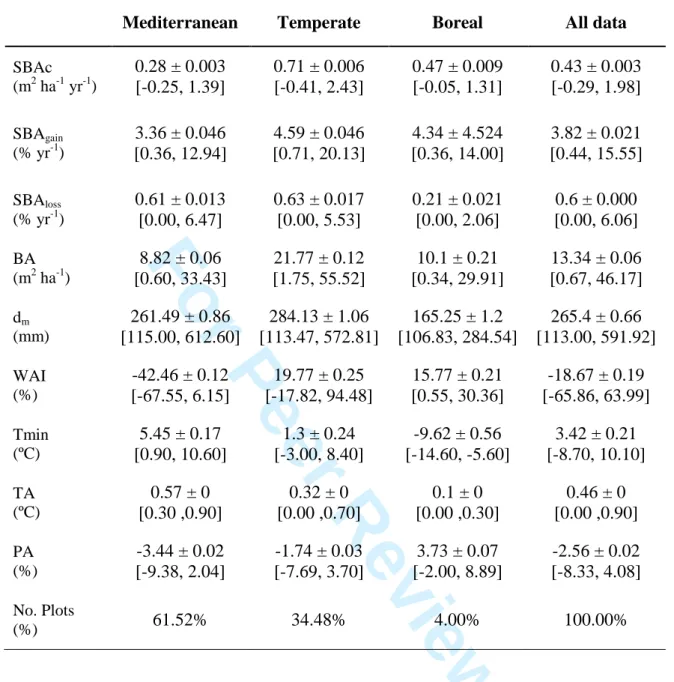
(39) Ecosystems. Ruiz-Benito et al. 36 806. Table 1. Summary statistics of the inventory plots. Mediterranean. Temperate. Boreal. All data. SBAc (m2 ha-1 yr-1). 0.28 ± 0.003 [-0.25, 1.39]. 0.71 ± 0.006 [-0.41, 2.43]. 0.47 ± 0.009 [-0.05, 1.31]. 0.43 ± 0.003 [-0.29, 1.98]. SBAgain (% yr-1). 3.36 ± 0.046 [0.36, 12.94]. 4.59 ± 0.046 [0.71, 20.13]. 4.34 ± 4.524 [0.36, 14.00]. 3.82 ± 0.021 [0.44, 15.55]. SBAloss (% yr-1). 0.61 ± 0.013 [0.00, 6.47]. 0.63 ± 0.017 [0.00, 5.53]. 0.21 ± 0.021 [0.00, 2.06]. 0.6 ± 0.000 [0.00, 6.06]. BA (m2 ha-1). 8.82 ± 0.06 [0.60, 33.43]. 21.77 ± 0.12 [1.75, 55.52]. 10.1 ± 0.21 [0.34, 29.91]. 13.34 ± 0.06 [0.67, 46.17]. dm (mm). 261.49 ± 0.86 [115.00, 612.60]. 284.13 ± 1.06 [113.47, 572.81]. 165.25 ± 1.2 [106.83, 284.54]. 265.4 ± 0.66 [113.00, 591.92]. WAI (%). -42.46 ± 0.12 [-67.55, 6.15]. 19.77 ± 0.25 [-17.82, 94.48]. 15.77 ± 0.21 [0.55, 30.36]. -18.67 ± 0.19 [-65.86, 63.99]. Tmin (ºC). 5.45 ± 0.17 [0.90, 10.60]. -9.62 ± 0.56 [-14.60, -5.60]. 3.42 ± 0.21 [-8.70, 10.10]. TA (ºC). 0.57 ± 0 [0.30 ,0.90]. 0.32 ± 0 [0.00 ,0.70]. 0.1 ± 0 [0.00 ,0.30]. 0.46 ± 0 [0.00 ,0.90]. PA (%). -3.44 ± 0.02 [-9.38, 2.04]. -1.74 ± 0.03 [-7.69, 3.70]. 3.73 ± 0.07 [-2.00, 8.89]. -2.56 ± 0.02 [-8.33, 4.08]. 61.52%. 34.48%. 4.00%. 100.00%. ee. rP. 1.3 ± 0.24 [-3.00, 8.40]. iew. ev. rR. No. Plots (%). Fo. 1 2 3 4 5 6 7 8 9 10 11 12 13 14 15 16 17 18 19 20 21 22 23 24 25 26 27 28 29 30 31 32 33 34 35 36 37 38 39 40 41 42 43 44 45 46 47 48 49 50 51 52 53 54 55 56 57 58 59 60. Page 36 of 56.