Application of imputation techniques in collaborative filtering based recommender systems

Texto completo

(1)Master In Computational and Mathematical Engineering Final Master Project (FMP). Application of Imputation techniques in Collaborative Filtering-based Recommender Systems Sandra Díaz Romo Supervisor: Agustí Solanas 07/2018. Signature of the director authorizing the final delivery of the FMP:.

(2)

(3) This work is subject to a licence of RecognitionNonCommercial- NoDerivs 3.0 Creative Commons.

(4) Alternative licences (choose any of the following and substitute the one of the previous page) To) Creative Commons:. This work is subject to a licence of AttributionNonCommercial-NoDerivs 3.0 of Creative Commons. This work is subject to a licence of AttributionNonCommercial-ShareAlike 3.0 of Creative Commons. This work is subject to a licence NonCommercial 3.0 of Creative Commons. of. Attribution-. This work is subject to a licence of Attribution- NoDerivs 3.0 of Creative Commons. This work is subject to a licence of Attribution-ShareAlike 3.0 of Creative Commons. This work is subject to a licence of Attribution 3.0 of Creative Commons B) GNU Free Documentation License (GNU FDL) Copyright © YEAR YOUR-NAME. Permission is granted to copy, distribute and/*or modify this document under the terms of the GNU Free Documentation License, Version 1.3 or any later version published by the Free Software Foundation; with no Invariant Sections, no FrontCover Texts, and no **Back-Cover Texts. To copy of the license is included in the section **entitled "GNU Free Documentation License". C) Copyright © (The author/to) Reserved all the rights. It is forbidden the total or partial reproduction of this work by any half or procedure, comprised the impression, the reprography, the microfilm, the computer treatment or any another system, as well as the distribution of copies by means of rent and loan, without the permission written of the author or of the limits that authorise the Law of Copyright..

(5) INDEX CARD OF THE FINAL MASTER PROJECT. Title of the FMP: Name of the author: Name of the TUTOR: Name of the PRA: Date of delivery (mm/aaaa): Degree: Area of the Final Work: Language of the work: Keywords. Application of Imputation techniques in Collaborative Filtering-based Recommender Systems Sandra Díaz Romo Agustí Solanas Juan Alberto Rodríguez Velázquez 07/2018 Master In Computational and Mathematical Engineering Imputation methods English Multivariate Analysis, Imputation methods, Recommender systems. Summary of the Work (maximum 250 words): This master thesis focuses on imputation methods as an approach to deal with the missing data problem. It’s common that big datasets contain missing values. However, their existence may suppose a problem, as most of the usual statistical techniques can’t be used and they may shadow important features, leading to the extraction of incorrect conclusions. In this context, imputation methods are statistical methods used to infer the missing values of a dataset using its intrinsic properties and the correlation amongst their variables. Several of these methods have been studied in detail and used in a recommender systems case study. Recommender systems main goal is to use the available information to generate personalized recommendations for each user. They usually work with a very sparse matrix, which complicates the task of obtaining useful recommendations. The studied imputation methods have been applied on a user-item rating dataset in order to compare their results and to be able to discern whether the recommender system is able to generate a better set of recommendations with their use. After the implementation of the methods, and the recommender system, and the extraction of accuracy metrics results, we have concluded that they produce a great improvement of the output in datasets with a percentage of missing data greater than 60%. It has also been noted in several occasions the importance of the election of an appropriate imputation method.. i.

(6) Abstract (in English, 250 words or less): This master thesis focuses on imputation methods as an approach to deal with the missing data problem. It’s common that big datasets contain missing values. However, their existence may suppose a problem, as most of the usual statistical techniques can’t be used and they may shadow important features, leading to the extraction of incorrect conclusions. In this context, imputation methods are statistical methods used to infer the missing values of a dataset using its intrinsic properties and the correlation amongst their variables. Several of these methods have been studied in detail and used in a recommender systems case study. Recommender systems main goal is to use the available information to generate personalized recommendations for each user. They usually work with a very sparse matrix, which complicates the task of obtaining useful recommendations. The studied imputation methods have been applied on a user-item rating dataset in order to compare their results and to be able to discern whether the recommender system is able to generate a better set of recommendations with their use. After the implementation of the methods, and the recommender system, and the extraction of accuracy metrics results, we have concluded that they produce a great improvement of the output in datasets with a percentage of missing data greater than 60%. It has also been noted in several occasions the importance of the election of an appropriate imputation method.. ii.

(7) Index. 1. Introduction 1.1 Context and justification of the Work 1.2 Aims of the Work 1.3 Approach and method followed 1.4 Planning of the Work 1.5 Brief summary of products obtained 1.6 Brief description of the chapters of the thesis. 1 1 1 2 2 3 3. 2. Missing data 2.1 Classification 2.2 Importance and approach. 4 4 6. 3. Imputation Methods 3.1 Listwise Deletion 3.2 Mean Substitution Method 3.3 Hot-deck Imputation Methods 3.4 Predictive Mean Matching 3.5 Multiple Imputation 3.6 Proposed Imputation Method. 7 7 7 8 8 10 10. 4. Recommender systems 4.1 Evaluation. 12 13. 5. Imputation methods in recommender systems 5.1 Motivation 5.2 Datasets 5.2.1 Poisson Dataset 5.2.2 Jester Dataset 5.3 Creation of MCAR data 5.4 Imputation methods 5.5 Creation of a recommender system 5.6 Evaluation criteria. 15 15 15 15 19 23 24 25 27. 6. Obtained results 6.1 Poisson Datset 6.1.1 Number of recommended items 6.1.2 Recall, precisión and F1-Score 6.1.3 Execution time 6.2 Jester Datset 6.2.1 Number of recommended items 6.2.2 Recall, precisión and F1-Score 6.2.3 Execution time. 28 28 28 29 32 34 34 35 38. 7. Conclusions. 40. 8. Glossary. 42. 9. References. 43. iii.

(8) List of figures. Figure 1: Poisson dataset histogram ........................................................................................................... 16 Figure 2: Poisson dataset ratings histogram per item ................................................................................. 17 Figure 3: Correlation matrix of Poisson dataset ......................................................................................... 18 Figure 4: 2D representation of the users in clusters using 5-Means and PCA ........................................... 19 Figure 5: Jester dataset histogram .............................................................................................................. 20 Figure 6: Jester dataset ratings histogram per item .................................................................................... 21 Figure 7: Correlation matrix of Jester dataset ............................................................................................ 22 Figure 8: 2D representation of the users in clusters using 7-Means and PCA ........................................... 23 Figure 9: Number of recommendations generated in Poisson dataset ....................................................... 28 Figure 10: Poisson dataset recall results ..................................................................................................... 29 Figure 11: Poisson dataset precision results ............................................................................................... 31 Figure 12: Poisson dataset F1-score results................................................................................................ 32 Figure 13: Poisson dataset execution time results ...................................................................................... 33 Figure 14: Number of recommendations generated in Jester dataset ......................................................... 34 Figure 15: Jester dataset recall results ........................................................................................................ 35 Figure 16: Jester dataset precision results .................................................................................................. 36 Figure 17: Jester dataset F1-score results ................................................................................................... 37 Figure 18: Jester dataset execution time results ......................................................................................... 38.

(9)

(10) 1 1.1. Introduction Context and justification of the Work. At the present time, which is marked by an impressive growth of the Information Technology, the possibility to seek and find a product that meets certain requirements, amongst millions of existing products all over the world, is just a click away. Revolutionary ideas, such as having the ability to buy or sell commodities over the Internet, also known as e-commerce, have become commonplace. On-line users get to compare thousands of products in real time as well as to read other users’ feedback or even give their personal feedback and rating for each product. In this context, the capability of creating personalized recommendations for each user in order to offer relevant products has gained a remarkable importance. Moreover, an optimization of the recommender systems’ accuracy is also being sought by vendors so they can make their products reachable for a larger audience. With the mentioned recommendation optimization, costumers are also able to reduce their search time for each product as they receive fitter products regarding their preferences. One of the problems that recommender systems have to face is the lack of enough information of the preferences of each user. Even though there are users that actively participate on giving feedback of the products, there is a larger number of them that are not rated. This fact makes the generation of recommendations more difficult. In this master thesis, imputation methods are reviewed as a potential solution to the missing data problem of recommender systems. Those methods use the intrinsic features of the available data in order to estimate a user’s opinion of each product. Thus, they provide the recommender a reconstruction of each user ratings, facilitating the generation of recommendations. In addition to the study of recommender systems in the e-commerce context and several imputation methods, a imputation method proposal can be found. The proposed method is aimed to be used in those datasets that contain variables expressed in several scales and with a probable existence of outliers.. 1.2. Aims of the Work. This thesis aims from both, a practical and a theoretical point of view, are • Understand the importance and consequences of missing data, specially from the perspective of recommender systems in the current context. • Theoretical study of several imputation methods: methodology, advantages and disadvantages. • Theoretical study of recommender systems: methodology, popular approaches used in the e-commerce context and evaluation. • Implement several imputation methods and a recommender system in order to provide recommendations for an actual rating dataset. • Analyze the obtained results and discern whether the use of imputation methods implies an improvement in the generated recommendations.. 1.

(11) 1.3. Approach and method followed. The strategy chosen for this master thesis has been to use a combination of a theoretical and a practical approach. On the one hand, the chosen theoretical approach is based on published papers and books about missing data, imputation methods and recommender systems. In which ways does missing data affect us in our daily basis, what are the most used imputation techniques, and why, or how do web pages find items that are likely to meet our expectations, are some of the questions that raise in the thesis starting point. On the other hand, since the chosen topic of study is an actual practical problem that’s being studied worldwide, as it affects several fields such as medical research or e-commerce, and it involves programming algorithms and working with statistical results, a practical approach has been found pertinent. It has consisted on choosing several imputation methods as well as a recommender system method and implementing them in order to test their performance. A statistical study of the chosen datasets and of the obtained results it’s also part of this approach. Both strategies, the practical and the theoretical one, offer a different point of view on studying the problem. The first one focuses on imputation algorithms and recommendation algorithms from a theoretical point of view: advantages and disadvantages of each method, creation of new algorithms, or optimization of the existent ones, whereas the second one focuses on the application of these methods on real datasets: implementing the methods, checking its computational performance, finding new ways of storing the data and evaluating the actual accuracy results. Both approaches are equally valid and a thesis could be based in just one of them, deepening more in the chosen one. In spite of that fact, the option of taking both approaches has been the chosen one due to the complete vision of the problem that it provides: allowing the study of the imputation methods advantages and disadvantages as well as testing their performance when they are used in recommender systems, checking the theoretical assumptions in the practical obtained results.. 1.4. Planning of the work. This thesis work has been divided into 3 phases: the theoretical phase, the practical phase and the presentation phase. Each of them can be identified in the Gantt chart by the green color, orange color and blue color respectively.. The theoretical phase is planned to last the first 4 months of the work, it begins on October, 15th and ends on March, 8th. It consists in doing a research on the selected topic, imputation methods,. 2.

(12) as well as on other related topics, such as missing data, recommender systems or evaluation metrics. This phase also consists in finding a suitable real dataset for the practical phase. A milestone has been set on the end of on this phase, marking the end of the research, which would mean that all the necessary information has been gathered. The practical phase is planned to take the next 3 or 4 months, it begins on February, 2nd and ends on June, 1st. It consists in implementing the recommender system and the imputation methods previously studied and testing their performance. It also consists in evaluating and representing the obtained results. For this phase, a previous work of preparing the coding software will be necessary. Two milestones are set for this phase: the first one marks the ending of the coding work and the second one marks the ending of the evaluation and representation of the obtained results, making way for a total dedication to the final phase. The last phase, the presentation phase, it consists in the writing of the documentation and the evaluation, as well as in the production of the thesis presentation. The last milestone, set on July, 10th, marks the ending of the thesis.. 1.5. Brief summary of the products obtained. In order to test the theoretical concepts studied, a recommender system will be imputed along with several imputation methods. This system, given a dataset and a specific user will return a list of personalized recommendations. After its implementation, it will be used to check the impact of using imputation methods and use a complete dataset as the input of the recommender.. 1.6. Brief description of the chapters of the thesis. The next chapters of the thesis can be divided in two groups: from chapter two to four, one can find the theoretical explanation of the thesis, as well as all the definitions of the key concepts studied, and, on chapters five and six, one can find the explanation of the methodology used in the practical part of the thesis and the obtained results. Chapter 2 contains an introduction to missing data: context, storing of data, definition, notation in a dataset and classification. One also can find the consequences of its appearance and, thus, why it is important to find a way to deal with it. Chapter 3 starts by providing the definition and the main purpose of imputation methods. The chapter is divided in sections, each of them containing a detailed explanation of an imputation method approach and its advantages and disadvantages. The proposed imputation method can be found in the last section. The main topic reviewed in Chapter 4 is recommender systems: importance in the on-line world, basic definitions, used strategies and the collaborative filtering approach. Several evaluation measures of the recommender systems accuracy are formally defined. Chapter 5 is focused on the theoretical explanation of the practical part of this thesis: an statistical study of the used datasets, the algorithm applied to create missing data, the chosen imputation methods and its configuration, the recommender system methodology and the evaluation criteria are the reviewed points. Finally, Chapter 6 contains the obtained results of the practical part. Those are graphics represented and used to reach to conclusions.. 3.

(13) 2. Missing data. In most research areas, gathering and analyzing data is an essential task to be fulfilled in order to comprehend the field of study and be able to make further investigation. Likewise, in most enterprises, this task is also essential in order to be able to analyze the current situation and to make the best decision possible given the current market context. There are diverse methods to bring data together, such as doing polls or interviews, taking measures using machines or doing experiments in a lab and writing down the observed results. Gathered data are usually treated to be stored in a tabular way, which we will refer to as dataset, to be analyzed using several statistical methods. In a tabular structure, the dataset can also be considered as an n × p matrix Y = {Yi, j } where i = 1, ..., n denotes the sample or individual and where j = 1, ..., p denotes a variable or feature. In other words, there are as many rows as samples, or individuals, and there are as many columns as measures of the features of each individual.  Y1,1 Y2,1   ..  .   Y =  Yi,1  ..  .   .  .. Yn,1. Y1,2 Y2,2 .. .. ... .... Y1, j Y2, j .. .. ... .... Yi,2 .. . .. . Yn,2. .... Yi, j .. . .. . Yn, j. .... .... ....  Y1,p Y2,p   ..  .   Yi,p   ..  .   ..  .  Yn,p. We say that a dataset contains missing data if some of its values are unknown. Those can be represented with a wildcard, i.e. an specific number to represent its missingness, or they can be left empty, using a null value. In this thesis we will be working with the statistical language R, in which unknown values are represented as NA. There are a lot of reasons that can cause values to be missing. For instance, if the dataset stores the answers of a statistical poll, missing values are the questions which had not been answered. If the dataset is a compilation of measures taken by a machine, missing values would be some of the features that it hasn’t been able to measure for some reason, such as a technical failure. Likewise, some of the data may be missing due to human error, for instance, in the lab case some of the samples could have been damaged during the experiments. Whatever its cause may be, missing data are a common feature in most datasets and, therefore, they must be taken into account before the dataset statistical analysis.. 2.1. Classification. There are several assumptions that can be made about missing data. In order to define them formally, let Y be the dataset tabular representation, a data matrix, formed by several variables X1 ,X2 ,...,Xn .  Y1,1  .. Y= .. Y1,2 .. .. .... Yn,1. Yn,2. ....   Y1,p ↑ ..  = X  1 . ↓ Yn,p. 4. ↑ X2 ↓. ... ... ....  ↑ Xn  ↓.

(14) Let Yobs be the set of those values of Y which are known and let Ymiss be the set of those values of Y which are missing. Thus, Y = (Yobs ,Ymiss ). Finally, let R be the matrix of missingness where ( 1 if Yi, j ∈ Yobs Ri, j = 0 if Yi, j ∈ Ymiss Missing data can be classified, regarding its causality, in one of the following types[1] . • Missing completely at random (MCAR). We say that a dataset missing data is MCAR if the probability of missing data of any variable Xi is unrelated to the value of Xi itself or to the value of any other set of variables of the dataset. Formally, it can be written as P(Ri, j = 0) = P(Ri, j = 0|Yi, j ) = P(Ri, j = 0|Yobs ) An example of MCAR missing data is when several samples of an experiment are not correctly conserved, so they are damaged and some of its features can’t be measured. The missing values in these samples are not related to the samples itself, nor any of their features, or to any other samples, but to a human error during the conservation procedure. • Missing at random (MAR). We say that a dataset missing data is MAR if the probability of missing data on a variable Xi is unrelated to its value after controlling for other variables in the analysis Xi1 ,...,Xim . That is, once the values of Xi1 ,...,Xim have been fixed. Formally, P(Ri, j = 0|Yi, j ,(Xi1 , j ,...,Xim , j ) = (ξ1 ,...,ξm )) = P(Ri, j = 0|(Xi1 , j ,...,Xim , j ) = (ξ1 ,...,ξm )) In other words, given an specific population of individuals, the MCAR assumption is given. Note that MAR assumption is weaker than MCAR. Consider a political opinion poll where the missing values come from people that refuse to answer and where there are some demographical areas that show a larger refusing rate. Missing data will fulfill a MAR assumption if, in each area, the missing values don’t depend on the demographics, that is, it’s not related to the area of the person that’s being interviewed. • Missing not at random (MNAR). We say that the dataset missing data is MNAR if the probability of missingness depends on the missing value itself. An exam question that was not answered by most of the students who took it in the last row of the class is an example of MNAR missing data if missing values are related to the position of the students in the class. If it’s taken the MCAR o MAR assumption, the dataset can still be considered as a valid representation of the population[1] . Whereas, if it’s taken the MNAR assumption, bias problems in its analysis are likely to appear. Note that an MCAR assumption of the missing data is not likely to be realistic. Most of the times, there’s a reason behind data’s missingness and figuring out why are those specific values missing is as important as the imputation process itself to achieve a good understanding of the data. 5.

(15) 2.2. Importance and approach. As the final purpose of the study of a dataset is to be able to gain knowledge about a specific field, it’s important to obtain reliable statements of the statistical study in order to avoid misleading conclusions. Missing data reduces the characterization of the population, as some of its features may be shadowed and, thus, it can distort the extracted conclusions. Statistically speaking, those distortions are the bias that missing data causes on the statistics. If, for instance, some of the largest values of a variable were missing, its mean would be much lower than it really is. For that reason, most of the statistical methods of data analysis are not content robust when dealing with missing data, as their statistics are easily affected. Clearly, as the number of missing values increases, the distortion within the data also increases. There isn’t a widely used convention about what is an acceptable percentage of missing data in a dataset and that’s partly because the percentage of missing data is not the only feature that must be considered. For instance, missing data patterns can have a greater impact on the statistics than their proportion, so there is not a rule of thumb and, ultimately, it depends on the specific dataset one is working with. A usual approach to deal with missing data is to delete those samples that contain missing values. However, as the proportion of missing data increases, the deletion of the samples becomes impracticable. This thesis goes in detail with an alternative approach: the use of imputation methods.. 6.

(16) 3. Imputation Methods. Imputation methods are a group of statistical methods that, given a dataset represented in a tabular way, are aimed at replacing each unknown value with a suitable one. Different methods follow different strategies with the intention to infer those values. The main idea behind the use of imputation methods is to use information of the known part of the dataset to make an estimate of the missing values. An important advantage that offer this family of methods is that, once all the missing values are imputed, the dataset is a complete one and standard data analysis methodologies can be used. The quality of the analysis and the reached conclusions will be directly related to the quality of the imputation of each value. Thus, a correct election of the imputation strategy to be used is crucial in order to obtain good approximations to the actual values. An imputation process that produces bad estimations can generate as much distortion in the data as the missing values themselves. A detailed explanation of some of the most used imputation methods, as well as some of its advantages an disadvantages can be found in the following sections of this chapter.. 3.1. Listwise Deletion. Although listwise deletion is not a proper imputation method, as missing values are not inferred, it’s still, by far, one of the most used methods in order to deal with missing data, so we’ve considered it worth to be mentioned. Listwise deletion, also known as complete case, consists in deleting all those samples, or individuals, which contain any missing value in any of its variables. This way, the statistical study is only done on the complete samples of the dataset. The main advantage of this method is its simplicity, as it’s not needed any special programming skill nor software to use it, and it’s useful when there are only a few individuals, or samples, which have missing values. In addition, complete case analysis methods can be used right away. Nevertheless, when the number of samples with unknown values is not negligible, the immediate consequence of deleting them is a reduction of the statistical power[1] , as all the available information is not used. Furthermore, it the data is not MCAR, estimates can be biased, as it’s possible that an entire population is being omitted from the study.. 3.2. Mean Substitution Method. Mean substitution is a simple imputation technique that consists in replacing each missing value with the mean of the known values of its respective variable. Formally, if Yi j ∈ Ymiss , its imputed value is calculated as[1] Ỹi, j =. ∑nk=1 Rk, j ·Yk, j ∑nk=1 Rk, j. where Rk, j are the respective values of the variable in the matrix of missingness R. One of the most important advantages of this method is the low computational cost it has because it’s only necessary to compute each variable’s mean.. 7.

(17) On the other hand, there are several disadvantages. It reduces the variability in the data because of the use of the mean value, as it’s repeated several times in each variable. It also weakens the covariance and correlation statistics in the data because this method ignores the relationships between variables.. 3.3. Hot-deck Imputation Methods. Hot deck imputation methods are a group of imputation techniques that aim to infer the unknown values of the samples, or individuals, of the data using information of the dataset from the most similar individuals to the one that’s being inferred. Given a specific sample that contains missing values, known as the recipient[2] , the main idea of this group of methods is to select one sample, or a group of samples, within the dataset which will be used to infer the recipient’s missing values. Those samples are known as donors[2] and, usually, are selected in terms of similarity with the recipient, i.e. in terms of distance. Each method proposes a specific methodology in selecting the recipient’s donors and in inferring the unknowns. Regarding the selection of donors, some of the methodologies that are being used include the use of distance functions or clustering methods, as the k-Nearest Neighbors methods, also known as k-NN, or the k-Means methods. On the other hand, regarding the process of inferring the missing values from the donors, we can distinguish two types of hot-deck methods[2] : • Deterministic hot-deck methods. Are those hot-deck methods that, once all the donors are selected, use a deterministic approach to infer the missing data, that is, use a closed formula to estimate the unknown value. For instance, using the mean, or another arithmetic expression using features of all the donors. Its also considered to be deterministic to select the recipient’s closest donor and use its value of the missing variable. • Random hot-deck methods. Are those hot-deck methods that, once all the donors are selected, use a random approach to infer the missing data. For instance, choosing one donor’s value randomly to infer the recipient unknown value of the same variable. Without considering which type of hot-deck method it’s being used, and to a greater or lesser degree, all of them share the advantage that the missing data its being imputed using information from within the dataset, so they intrinsically use the existent relationships (correlations, etcetera) between variables without predefining them nor making any initial assumption about the data. In spite of that, it has to be reminded that those methods depend on the choice of metric used to match donors to recipients, so they are far to be assumption-free methods. Furthermore, they don’t provide good approximations for outliers, as there are not really similar samples within the dataset.. 3.4. Predictive Mean Matching. The Predictive Mean Matching method[3] , also denoted as PMM method, is a random hot-deck method that consists in retrieving actual dataset values from the nearest observed individuals. In PMM, the recipient’s nearest individuals in a specific variable are those individuals that have a known variable value and which linear regression estimated value for the imputed variable is similar to the recipient’s linear regression estimated value.. 8.

(18) Given a dataset with data matrix Y ∈ Rn×p , let Yi,miss be the value that’s going to be imputed and, therefore, let Xmiss be the variable which values are being imputed from. Finally, let ~X = (X1 , X2 , . . . , Xt ) be a set of variables of the dataset selected to be used to estimate Xmiss as a linear combination of them, that is, Xmiss = β1 X1 + β2 X2 + · · · + βt Xt + ε where ~β = (β1 , β2 , . . . , βt ) are known as the regression coefficients and where ε is the error term. The Predictive Mean Matching method follows the next steps[3] . • Use the Regression Imputation method in order to obtain the regression coefficients β1 , β2 , . . . , βt . ~ – Using a least squares-based linear regression, obtain the estimates β̂ = (βˆ1 , βˆ1 , . . . , β̂t ), ~ ~ ~ σ̂ (β̂ ) and ε̂. Where β̂ are the estimates of the regression coefficients ~β , σ̂ (β̂ ) denotes the estimate of the variance of the coefficients estimate and where ε̂ is the estimate of the error term. – Given the previous estimates, regression coefficients β~∗ = (β1∗ , β2∗ , . . . , βt∗ ) are ex~ tracted from a multivariate normal distribution located at µ = β̂ and with covariance 2 ∗ ∗ matrix Σ = σ 2 (~X T ~X)−1 , where σ 2 = ε̂g , being g a χ 2 variate with nobs − t degrees of freedom, where nobs is the number of known observations of Xmiss . The extraction of the regression coefficients using a multivariate normal distribution is essential to produce enough variability in the imputed values. – Given β~∗ = (β ∗ , β ∗ , . . . , β ∗ ), the variable Xmiss can be modeled as 1. 2. t. Xmiss = β1∗ X1 + β2∗ X2 + · · · + βt∗ Xt . • Given the modeling of the variable Xmiss , all its values, having a known or unknown value, are estimated using the formula Ŷl,miss = β1∗Yl,1 + β2∗Yl,2 + · · · + β p∗Yl,t where l ∈ {1, . . . , n}. • A set {~Yl1 ,~Yl2 , . . . ,~Ylk } of the k0 nearest individuals to the individual ~Yi is extracted. Those 0 individuals are obtained getting the k0 minimum values of |Ŷi,miss − Ŷl,miss | where Yl,miss ∈ Yobs , i.e. is a known value. • Finally, one of the individuals of the set {~Yl1 ,~Yl2 , . . . ,~Ylk } of donors is randomly chosen, let 0 it be ~Yl , and its value Yl ,miss is used as the new value. j. j. Ỹi,miss = Yl j ,miss The distinctive point of the Predictive Mean Matching method is that it uses a linear regression of the variables in order to study its similarity, not to infer its value. Furthermore, the fact that imputed values are real values borrowed from real data individuals maintains the upper and lower bounds. In spite of these facts, the PMM method is only useful when a linear relationships is believed to exist between the variables. Otherwise, the result would be a bad modeling of the missing variable and, thus, a wrong election of the similar individuals, which can finally result in a bad imputation value.. 9.

(19) 3.5. Multiple Imputation. Several imputation methods that we’ve explained up to this point, as the Predictive Mean Matching or the Random Hot-deck methods, include a random selection from the pool of donors. The fact of choosing randomly, carries uncertainty about the imputed values. With the motivation of narrowing this uncertainty, the Multiple imputation method provides a useful strategy based on three main steps[2,4] : 1. Imputation. Given a dataset which contains missing values and which is stored in a matrix Y, the multiple imputation method generates a set of m complete datasets {Y1 , Y2 , . . . , Ym } by using the same random imputation method. Usually, m takes value from 3 to 5. 2. Analysis. Each of the m datasets extracted from the previous step are analyzed by using standard procedures, such as the computation of some statistics. 3. Pooling. After the conclusions extracted from the analysis of the datasets, the obtained results are combined from the m different datasets into a final one. Multiple imputation doesn’t attempt to estimate each missing value through simulated values, as deterministic hot-deck methods do, but to represent a random sample of the missing values. This results in valid statistical inferences that properly reflect the uncertainty due to missing values[4] , as well as in a reduction of the bias and an increase of the precision. However, an important disadvantage of multiple imputation is that it’s a time consuming method due to the multiple iterations in the datasets and their respective analysis. It’s also required a statistical expertise to understand the analysis step.. 3.6. Proposed Imputation Method. From the advantages and disadvantages studied in the previous imputation methods, a variant of the k-NN hot-deck imputation method has been proposed in this thesis. The k-NN hot-deck[5] method consists in using a mean substitution method on the dataset to compute the k Nearest Neighbours of an element, i.e., those k elements which are closer in terms of similarity. In the random version of this method, one of the k donors is randomly selected to impute each missing value of the recipient. Our proposal is a change in the similarity computation, that is, changing the distance function to be used. Usually, a preliminary imputation method is used to fill the missing values of the dataset and, then, a distance is used to compute the distance matrix of the elements,   d1,1 d1,2 . . . d1,p  .. ..  D =  ... . .  dn,1. dn,2. .... dn,p. where di, j = di, j is the distance between the users i and j. Instead of this approach, it has been considered to compute the distance between the users using just the real information contained in the dataset, that is, comparing just the common known values. In addition, we’ve considered using Mahalanobis instead of the Euclidian distance. Given two points ~x,~y ∈ R p , the Mahalanobis distance between ~x and ~y is defined as q dM (~x,~y) = (~x −~y)T S−1 (~x −~y). 10.

(20) where S is the variance-covariance matrix of the dataset. This distance considers the correlations between the variables when computes the distance between two points of the space. As the variance-covariance matrix, S, is required to compute the Mahalanobis distance but there’s still missing values in the dataset, it has been considered to use a preliminary hot-deck method to fill the data in order to compute S. The reason of this method election is that hot-deck methods conserve the existent relationships between the variables. Thus, the distance between two points~x and~y of a dataset is defined as the Mahalanobis distance[6] of their common elements. Formally, given two points ~x, ~y ∈ R p which have r common known values, let ~x∗ , ~y∗ ∈ Rr be the vectors with ~x and ~y common known variables. Given the imputed variance-covariance matrix S, let S∗ ∈ Rr×r the matrix containing the information of covariance and variance of ~x and ~y common known variables. This way, the distance d∗ between ~x and ~y is defined as q x∗ −~y∗ ) dM∗ (~x,~y) = dM (~x∗ ,~y∗ ) = (~x∗ −~y∗ )T S−1 ∗ (~ With the purpose of avoiding false similarity computation, this distance has been defined such that if ~x and ~y do not have a minimum number of elements in common, then dM∗ (~x,~y) = ∞ The minimum number of elements in common has been controlled using a tolerance percentage of common elements. Note that, this way of measuring distance implies that some of the distances will be measured with a greater number of variables in some of the individuals, but the point of its use is to measure how similar two samples using the available information. From this point on, the method follows the same steps as the k-Nearest Neighbours Imputation Method: for each point, it computes its k-Nearest Neighbours and selects one of them randomly to use its value to infer each missing value. Even though the use of Mahalanobis distance ensures a measure of the similarity between users without scale distortion by taking into account relationships between the variables and it’s really useful in detecting outliers, it also implies an increment of the computational cost that should be analyzed to determine whether this method is computationally affordable.. 11.

(21) 4. Recommender systems. Nowadays, the possibility of seeking between an incredibly large amount of products, adjusting the search to our preferences, is just a click away. Furthermore, users are able to provide feedback about any product. Thus, the fact of being able to provide personalized recommendations has taken a special importance. Recommender systems are information filtering systems which final aim is to create a list of recommendations by predicting the rating that an specific user would give to all the unrated, or unseen items[7] . The list is formed by those items that have obtained the greater predicted rating, or with the top-N rated items. In other words, recommender systems estimate the likeability of a large number of products and offers those items which are likely either to be useful in the search or to be liked by the user. These systems are particularly useful in the context of e-commerce for both sides, customers and vendors. Customers can find a larger number of similar products in less time, which is also convenient for vendors, as their products have a greater probability to be exposed to possible customers, leading usually to an improvement of those products’ sales. Recommender systems are also widely used in single-themed web pages about books, films, recipes, TV shows, etcetera. In order to create the list of recommendations for a user, those systems usually use information about • the user’s feedback. Recommender systems use the information contained in ratings that the user has given to different items. • the user’s behaviour. Instead of explicit feedback, these systems can use information about the user’s interactions, such as how many times a user has viewed the details of a certain item, or a list of the items searched in the last few days. • other users feedback or actions. Recommender systems usually seek other users with similar tastes, that is, similar ratings, in order to find items that could interest the user. • similar items. They can also use information about items with the same features, or classification, that the ones that the user has rated positively. A typical approach to produce a list of recommendations is through collaborative filtering[7] . This methodology is based on using the ratings provided by multiple users to make recommendations. Collaborative filtering is based on the idea that, in general, if two users had similar tastes in the past, they will also coincide in the future. In other words, the observed ratings between similar users are often highly correlated across various items. Ratings are usually stored in a matrix and, in general, there will be a much larger number of unrated items than rated ones for each user, so it will be a very sparse matrix. In fact, one of the main problems that recommender systems struggle with is that they work with this type of matrix, which makes it harder to create a good set of recommendations due to the lack of information. Formally, let’s consider a ratings dataset Y, which takes the form of a very sparse matrix.   Y1,1 Y1,2 . . . Y1,p  .. ..  Y =  ... . .  Yn,1 Yn,2. .... Yn,p. In this context, each column of the matrix represents an item and each row represents a user. Thus, the element Yi, j represents the rating that the user i has given to the item j. For that reason, we will refer to this matrix as the user-item matrix[8] . 12.

(22) Given the user-item matrix Y and a specific user i, the recommender system will return a set of items j1 , j2 , . . . , jk ∈ {1, 2, . . . , p}, where k can vary depending on the methodology used. Some of them return a constant number kc of recommendations, which are usually the top-kc rated ones, whereas others return only those items that have an estimated rating above a predefined threshold.. 4.1. Evaluation. Recommender systems that use different methodologies can generate very different recommendation lists even though they have the same input. For that reason, in order to choose a recommender system for a specific dataset, it’s useful to have a set of metrics that help us understand different aspects about the performance of each one. Taking into account that the most important result for the final user is to receive a good set of recommendations, a widely accepted methodology to test a recommender performance is to measure its accuracy, that is, to measure the accuracy of each recommended item. In order to define those metrics, some basic concepts will be defined formally. Let R̂ be a recommender system that given a user-item matrix Y and a specific user i, returns a set of recommended items { j1 , j2 , . . . , jk }. That is, R̂(i, Y) = { j1 , j2 , . . . , jk }, where R̂ : {1, 2, . . . , n} × Rn×p −→ {1, 2, . . . , p} × . . . × {1, 2, . . . , p} k). We say an item j is a relevant item when it is a good recommendation, that is, when its rating given by user i is greater than a given threshold t∗ . That is, item j is relevant for user i ⇔ Yi, j ≥ t∗ Let Vi denote the set of relevant items for user i. Threshold t∗ is usually set depending on the rating scale and the desired level of confidence of the recommendations. For instance, if each item can be rated from 0 to 5, a possible threshold could be 2.5 to obtain a medium level of confidence. We say an item j is a recommended item for user i when its given by the recommender system. That is, item j is recommended for user i ⇔ j ∈ R̂(i, Y). Given these basic definitions, we’re now able to introduce two of the most used accuracy metrics in recommender systems evaluation: precision and recall. Precision is defined as the proportion of recommended items that are also relevant. That is, Precision =. |Vi ∩ R̂(i, Y)| |R̂(i, Y)|. In a more intuitive way, it answers the question ”How many recommended items are actually relevant to the user?”. Recall is defined as the proportion of relevant items that have been recommended. That is, Recall =. |Vi ∩ R̂(i, Y)| |Vi | 13.

(23) In a more intuitive way, it answers the question ”How many relevant items have been recommended?”. In both measures, if |R̂(i, Y)| = 0 or |Vi | = 0, that is, there aren’t recommended items or relevant items respectively, then precision and recall have the value 1. That’s because given 0 recommendations, we do not have any recommended item that is not relevant, so precision is 1. Likewise, given 0 relevant items, we do not have any relevant item that is not identified. Even though precision and recall provide really useful information, the fact of having two metrics can make the election between several recommender systems harder, specially when they have obtained very different values in each metric. For instance, the election between a recommender system R̂1 with a high value of precision and a lower value of recall and a recommender system R̂2 with a high recall and a lower precision is not always trivial. In these cases, an interesting metric to consider is the F1-Score. The F1-Score is defined as the harmonic mean of precision and recall. F1-Score =. 1 recall. precision · recall 2 = 2· 1 precision + recall + precision. By definition, F1-Score considers both metrics to compute its score. This way, its easier to compare the performance of different recommender systems. In spite of this fact, a higher F1-score doesn’t necessarily mean that a recommender is better. It ultimately depends on each specific case, where recall could have more importance than precision or vice versa.. 14.

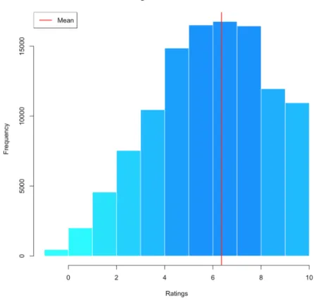
(24) 5. Imputation methods in recommendation systems. This thesis case of study consists in testing the effects of using imputation methods in recommender systems. In other words, on studying whether doing a previous imputation of a user-item matrix that comes from a rating dataset, improves the recommender system performance in terms of accuracy. Without going yet into greater detail, an algorithm is applied to a complete dataset to obtain a missing data version of itself. The dataset which contains missing data and its imputed datasets, created by applying different imputation methods, are used as the input of a recommender system. Finally, the obtained recommendation lists for each user are evaluated in terms of precision and recall in order to extract conclusions. The programming language R, in conjuction with the Rstudio software, has been used to codify the imputation methods, the recommender system and the posterior evaluation tests.. 5.1. Motivation. One of the main problems of recommender systems is that they usually work with a very sparse user-item matrix, since there are more items than items rated by each user. This fact deepens when users don’t rate the items even if they’ve interacted with them, for instance, bought them, eaten them or seen them. This absence of available data makes it harder to create a good set of recommendations as it’s more difficult to determine whether two users have similar preferences. Through the use of imputation methods, information within the dataset is used to produce an estimate of the ratings of each user, trying to figure out the likes and dislikes of each of them. Once the imputation process is over, and the user-item matrix is a dense one, the recommender system will have much more information to work with and to generate the list of recommendations. It’s worth noting that, as much as an imputation method can help a recommender system, it can also mislead it as it introduces certain levels of noise in the data due to the uncertainty generated by the missing values. Thus, in this problem, choosing an adequate imputation method for the dataset is as important as choosing an adequate recommender system.. 5.2. Datasets. Datasets used in the practical part of this thesis will be described and analyzed in this section. Note that they are complete rating datasets, that is, they do not contain missing values, as our purpose is to be able to evaluate the recommender system performance. Thus, the statistical analysis methods can be used in the usual way. 5.2.1. Poisson Dataset. The first dataset used, that has been named Poisson dataset after the distribution that has been used to create it. It’s a small R built-in dataset consisting of the ratings of 7500 users regarding 15 items, that is, containing a total of 112500 ratings. Those, are integers that take a value from 0 to 10. This dataset was created in order to do preliminary tests of the implemented code of the imputation methods and the recommender system before using a real-world dataset. In order to populate the user-item matrix, a combination of Poisson distributions have been used. The election of this distribution has been motivated by the fact that it returns integer numbers based on an occurrence rate and independently of the last number obtained. 15.

(25) Ratings of each item have been created independently by using a combination of three Poisson distribution outputs, each one of them configured with a different median number of occurrences λ which has been chosen randomly between values 2.5 and 8. In order to have a better understanding of this dataset and, to understand why some imputation methods work on it better than others, a statistical analysis can be found hereunder. The main aim of the exploratory analysis of the dataset is to provide a complete vision of the data. In this case ratings, items and users will be checked separately. On the right, a histogram of the ratings of Poisson dataset can be found. In this case, the mean of all the ratings has a value of 6.35. It can be seen that the most repeated ratings are from 5 to 8, being 7 the most repeated one with a total of 16762 ratings.. Figure 1: Poisson dataset histogram Ratings under 3 barely get to have 5000 ratings each one and there are more than 10000 ratings with value 9 and 10. It is also interesting, apart from seeing the overall results of the ratings, doing the same analysis on each one of the items in order to discover patterns, such as an item that has a really low ratings coming from all users or items in which users have divided opinions and have either very low or very high ratings.. 16.

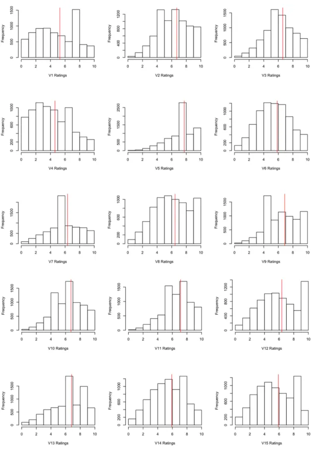
(26) Figure 2: Poisson dataset ratings histogram per item. 17.

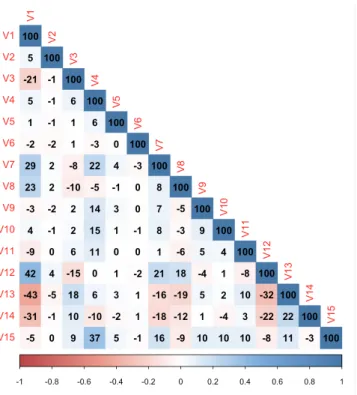
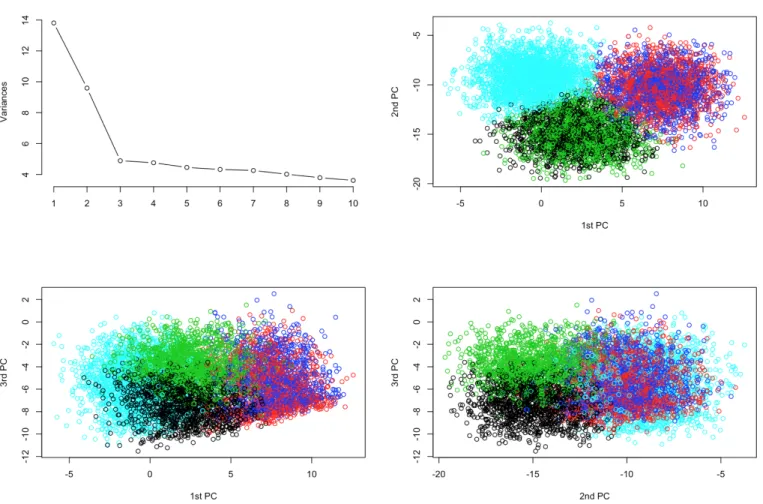
(27) One can see that, for instance, in items V5 and V7, most of the users have given the same rating, 8 and 5 respectively, whereas in other items, such as V4, V14 or V15, there exist a fair distribution between several ratings. In general, all items have a mean rating score greater than 5, being V5 the best rated item and V4 the worst rated one in mean terms. Another useful aspect to check is the linear relationship existing between the items, that is, knowing whether there is a correspondence between two items’ ratings. For instance, if a high rating in item A usually comes with a low rating in item B.. Figure 3: Correlation matrix of Poisson dataset As it can be seen in the correlation matrix of Poisson items, where values have been expressed in terms of 100 · %, most of the items don’t show a linear relationship, as their correlation items take values between -10 and 10. Two remarkable relationships are between items V1 and V12 and V1 and V13, having the most high positive and negative linear correlation.. Lastly, k-Means algorithm with k = 5 has been used in order to cluster users in several groups according to their ratings. Using the PCA method, the users’ ratings have been represented in several plots as bi-dimensional points using their corresponding Principal Components values.. 18.

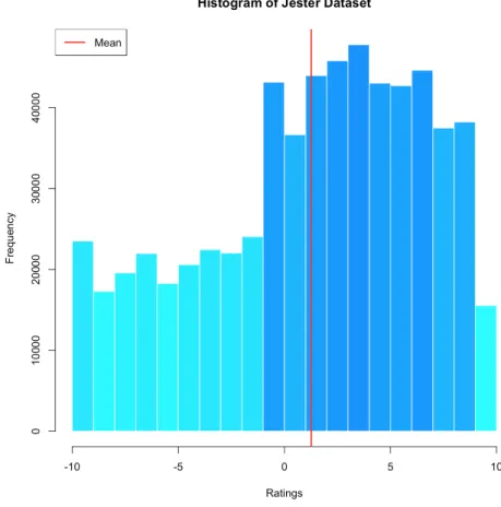
(28) Figure 4: 2D representation of the users in clusters using 5-Means and PCA The first three Principal Components have been chosen as they are the ones that have a greater value of variance, and therefore they explain a greater portion of the variability of the data, as it can be seen in the top-left plot. Looking carefully to the rest of plots, one can count a total of 4 different groups of users, as the blue and the red ones can be considered the same because they share the same area in all the plots. For instance, it can be seen that the green and black groups are different even they share the same space in the top-right plot because of the bottom left plot, where they correspond to different values of the third Principal Component even if they share values of the second Principal Component. 5.2.2. Jester Dataset. Jester dataset[9] is a real-world dataset consisting of 4.1 million anonymous ratings of 100 jokes from 73.421 users. Ratings were collected between April 1999 and May 2003, taking real values between -10 and 10. Missing ratings are represented with the number 99. In this thesis, a subdataset, consisting on the ratings of 23500 users that have rated 36 or more jokes, has been considered. Jester dataset is stored like a user-item matrix in a CSV format, so there it hasn’t been necessary any special treatment of the data. In order to obtain a complete dataset, a total of 28 jokes (V6, V8, V14, V16, V17, V18, V19, V20, V21, V22, V28, V30, V33, V36, V37, V43, V49, V50, V51, V54, V55, V57, V62, V63, 19.

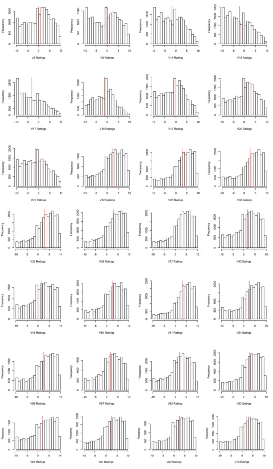
(29) V66, V67, V69 and V70) were considered as they where rated by the majority of the users, obtaining a final complete dataset consisting of ratings from 22454 users. As with the Poisson dataset, an initial exploratory analysis will be made in order to obtain a global vision of the Jester dataset and to be able to regarding conclusions regarding the application of imputation methods on it. A histogram of the ratings of the dataset can be seen in Figure 5.. Figure 5: Jester dataset histogram Jester dataset mean, taking into account all the ratings, has a value of 1.26. It can also be seen that values from -1 to 9 are the most frequent ones, having more than 35000 ratings in each integer interval, and that the less repeated values are those greater than 9. Ratings with values from -10 to -1 have a frequency of approximately 20000 ratings per integer interval. Individual ratings histograms can be found on Figure 6. Except for jokes V17, V18 and V21, a wider range of ratings can be observed in each joke since real values are being used to evaluate them, so there is a greater chance of variability in the scores between users even if they have, in general, the same opinion. Note that a big portion of jokes, from V22 to V70 have an approximately normal distribution shifted to the right as their mean is greater than 0, this can be seen specially on the two last rows of histograms. In spite of this fact, there are also jokes, such as V8, V14 or V20, that have as many positive ratings as negative ones, so their mean values are near to 0. 20.

(30) Figure 6: Jester dataset ratings histogram per item 21.

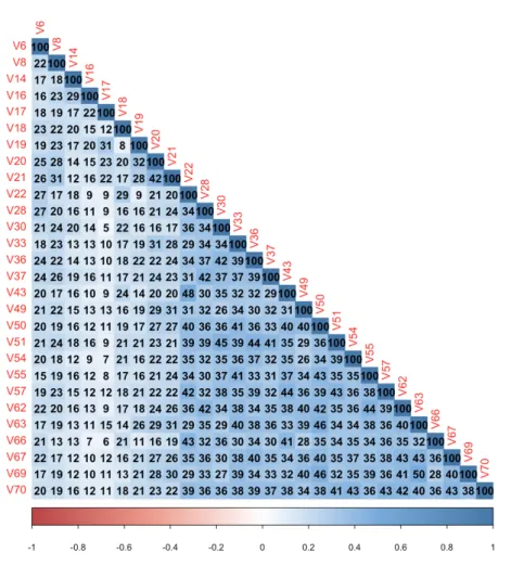
(31) Since PMM imputation method, based on linear relationships between variables, is going to be applied, the correlation matrix of the dataset has been computed and represented on Figure 7. Correlation values are expressed in terms of percentage from 0 to 100.. Figure 7: Correlation matrix of Jester dataset Note that all the linear relationships between the jokes, in an stronger or weaker degree, are positive. Therefore, high values of a joke A implies high values of a joke B and low values of A implies low values of B, rather than the other way around. Furthermore, one can distinguish between two trends in the computed correlation values. First 9 jokes, from V8 to V21, show a weaker linear relationship with all the other jokes, with values from 5 to 25. The correlation coefficients from jokes V22 to V70 are stronger, taking values from 30 to 45. Those last jokes are the ones that have a similar, and approximately normal, distribution of the ratings.. 22.

(32) Figure 8: 2D representation of the users in clusters using 7-Means and PCA Lastly, a k-Means with k = 7 has been used to cluster users in 7 independent groups. In order to do so, PCA algorithm has been used to represent them according to their values in the first and second Principal Components. The election of the first two PC has been motivated by their variance values: it can be seen in Figure 8 that they are the two PC that represent a greater portion of the variance of the data. Well defined divisions can be seen between the groups depending on the values of the first and second PC. All the users, except those that pertain to the green group, are divided depending on having a value of the second PC greater or lower that -5. At the same time, divisions are clear between different ranges of values of the first principal component.. 5.3. Creation of MCAR data. In order to test the performance of a recommender system when it works with different levels of uncertainty, datasets with several percentages of missing data, from 10 to 85%, have been generated from the complete datasets described in the previous section. Subdatasets of 150, 250, 500 and 750 users have been extracted from each dataset by selecting randomly, one by one, the specified number of users. The recommender system will work with this subdatasets instead of with the complete datasets in order to calculate the computational cost of each one of the imputation methods and to find out whether the number of users affects the recommender results. Given a complete dataset Y ∈ Rn×p and a missing data percentage pm , a MCAR dataset Y pm ∈ Rn×p is created by randomly selecting pairs [i, j], where i ∈ {1, 2, . . . , n} and j ∈ {1, 2, . . . , p}, so each pair represents a position in Y, and erasing their respective values in the user-item matrix. In R, this last step is done by assigning the value NA to each of the selected elements of the matrix. The number of pairs [i, j] depends on the percentage pm following the rule |[i, j]| = bn · p · pm c where n and p are the number of rows and the number of columns of Y respectively.. 23.

(33) Algorithm 1 Creation of an MCAR dataset 1: procedure CREATE MCAR DATASET 2: Y ← user-item matrix 3: pm ← missing data percentage 4: 5: 6: 7:. n ← num rows matrix Y p ← num columns matrix Y ind ← 1. 8: 9: 10: 11: 12: 13:. while ind < floor(n · p · pm) : i ← random integer between 1 and n j ← random integer between 1 and p Y [i, j] ← NA ind ← ind + 1 end while. 14: 15: 16: 17: 18:. return Y end procedure. 5.4. Imputation methods. To each MCAR subdataset used as the user-item matrix for the recommender system R̂, which comes from either Poisson dataset or Jester dataset and has a pm percentage of missing data, four imputation methods will be applied in order to obtain 4 complete versions. The imputation methods and their respective configurations are the following. • Mean substitution imputation method. This imputation method doesn’t require any configuration. • Hot-deck imputation method. The selected hot-deck method applies the previously mentioned imputation method, mean substitution, to the MCAR dataset in order to obtain a preliminary complete version. This complete version is needed to apply k-means algorithm to the dataset. k-means algorithm is a clustering algorithm which final aim is to divide the provided observations in k groups. Each observation pertains to a single group. Given a set of n observations ~o1 ,~o2 , . . . ,~on ∈ R p , k-means algorithm assigns each observation to its nearest centroid ~c1 ,~c2 , . . . ,~ck in terms of distance. Then, centroids are recomputed to be the mean of the elements of its group and the observations are reassign to their corresponding nearest centroid. This algorithm goes on until there are no changes in the groups. There are several methods to choose the initial centroids, for example, they can be k of the n observations. Once k-means has been applied, given a user i which belongs to a group ki , each of its missing values are randomly chosen from one of the other users of the same group which have a known rating. In case that all the users of the group have a common missing rating for an item, the imputed value in the initial mean substitution imputation is used.. 24.

(34) In this method, k has been set to 45 to avoid groups with a large number of users. The reason behind is that the estimated values are being randomly chosen, so the existence of groups with large cardinalities could make that some of them contain users that are not similar in its preferences and thus, the chosen value wouldn’t be a good estimation for i’s rating. • PMM-based Multiple Imputation method A multiple imputation method which uses the Predictive Mean Matching, also denoted as PMM, in each iteration has been chosen[10] . The value of m has been set to 3 so the method performs three imputations of the dataset. • Proposed method. In this thesis proposed method, the value of k has been set to 3 for the k-Nearest Neighbours method. The reason for this election is the same that the one explained in the hot-deck method: as the estimated rating will be one of the nearest neighbours, we want to ensure that they are the most similar, in terms of preferences, to the user. Note that all the selected methods preserve the rating’s boundaries. That is, the estimated values can not be greater that the maximum rating nor smaller that the minimum rating. This fact must been taken into consideration because it could affect the recommender system if it uses a threshold based on the ratings boundaries in order to determine if an item should be recommended or not.. 5.5. Creation of a recommender system. In this thesis case of study, it has been considered a recommender system R̂, defined as a function R̂ : {1, 2, . . . , n} × Rn×p −→ {1, 2, . . . , p} × . . . × {1, 2, . . . , p} k). based on collaborative filtering in order to produce a list of recommendations for any given user. Formally, given a user i and a dataset Y, recommender R̂ follows the next steps in order to obtain a list of recommended items R̂(i, Y) = { j1 , . . . , jk }. 1) Compute i’s Pearson correlation coefficient with the other users. Pearson correlation coefficient, ri1 ,i2 , between two users i1 and i2 , with ratings~x = (x1 , x2 , . . . , x p ) and ~y = (y1 , y2 , . . . , y p ) respectively, is defined as[8] p. ri1 ,i2 = q. ∑ j=1 (x j − x̄)(y j − ȳ) q ∈ [−1, 1] p p ∑ j=1 (x j − x̄)2 ∑ j=1 (y j − ȳ)2. where x̄ and ȳ are ~x and ~y means respectively. For instance, x̄ = 1p ∑ pj=1 x j . This coefficient is a measure of the linear correlation between two users and has values between -1 and 1. A value of 1 implies a perfect positive correlation, that is, a linear relationship between ~x and ~y where ~x increases as ~y increases. Likewise, a value of -1 implies a perfect negative correlation, that is, a linear relationship between ~x and ~y where ~x increases as ~y decreases. 25.

(35) Finally, a value of 0, denotes that there’s not a linear relationship between the users. 2) Obtain the k-Nearest Neighbours of i in terms of similarity. That is, those k users that have obtained a greater Pearson correlation coefficient with i, as we want the most similar users in terms of rating items. Only users with a positive correlation coefficient will be considered, thus, the final number of neighbours may be smaller than k. Value k = 5 has been chosen for the recommender system R̂ so a set of 5 neighbour users {i1 , i2 , . . . , i5 } will be obtained for i. Each of the neighbours ratings will be denoted as ~xim = (xm1 , . . . , xm p ), where m ∈ 1, . . . , 5. 3) For each missing value of the user i, compute a weighted average of the neighbours ratings as the estimation of the rating of i. Given a item j which user i has not rated, that is, has a missing value, the estimated rating x̃ j is  k  ∑m=1 ri,im · xm j · δm j     ∑k r · δ mj m=1 i,im x̃ j =      q. if ∃ m such that δm j 6= 0. if δm j = 0 ∀m. where q is the minimum rating value, in order to discard the election of item j as a recommended one, and where δm j is defined as δm j. ( 1 = 0. if Ym j ∈ Yobs if Ym j ∈ Ymiss. ∀m. To sum up, the estimated rating for each item is the weigthed average of those neighbours ratings which have a known value. Note that the weights are Pearson correlation coefficients, which take values in [−1, 1]. 4) Recommend those items that are relevant. In other words, return only those items that have obtained an estimated rating above a given threshold. Note that the number of recommendations may vary between users. In the Poisson dataset, the threshold has been set to 4 so R̂ recommends all those items that have estimated to score a minimum of this value. Likewise, in the Jester dataset, the threshold has been set to 0 so R̂ returns all those items that are estimated to have a positive rating.. 26.

(36) 5.6. Evaluation criteria. In order to test the recommender system performance and, therefore, the practicality of doing a previous imputation of the datasets, the following evaluation measures have been calculated. - Number of recommended items - Precision - Recall - F1-score - Computational time As there are random elections in both, some of the imputation methods and the recommender system, several runs have been made to ensure obtaining representative results. From the initial complete datasets, up to 25 subdatasets of 150, 250, 500 and 750 users have been extracted randomly, turned into MCAR subdatasets and imputed 4 times. Thus, 5 different subdatasets have been used to generate recommendations for each user in each run, making a total of 18750, 31250, 62500 and 93750 recommendation lists generated for the cases of 150, 250, 500 and 750 users respectively. Thus, more than 200000 recommendation lists have been generated in total. From each recommendation list, precision, recall and the total number of recommended items have been computed. The final values have been obtained by doing a mean of each list precision, recall and the number of recommended items respectively. The F1-score measure has been obtain by computing an harmonic mean of the final results of precision and recall. Using the same methodology, the necessary execution time to create each list have been extracted by doing a mean of all the execution times. This measure has been consider to study the computational cost of each imputation method as well as the practicality of their use in a real time computation.. 27.

(37) 6. Obtained results. This last chapter focuses on the presentation and the extraction of conclusions of the results obtained in the practical part of the thesis, which has been explained in detail in the previous one. The chapter has been divided into two sections, each for one of the two different datasets that have been tested. In each section, accuracy metrics and performance metrics are discussed. Each generated plot of each metrics consists of 4 individual plots that represent the obtained results depending on the cardinality of the subdataset, that is, the number of users selected, which take values in 150, 250, 500 and 750.. 6.1. Poisson dataset. 6.1.1. Number of recommended items. As the recommender system uses a predefined threshold in order to know if an item should be recommended or not, instead of returning the top-N items, a metric to take this fact into account is the length of the generated recommendation lists. The number of recommended items depending on the number of users of the subdataset and depending on the percentage of missing data can be found on Figure 9.. Figure 9: Number of recommendations generated in Poisson dataset.. 28.

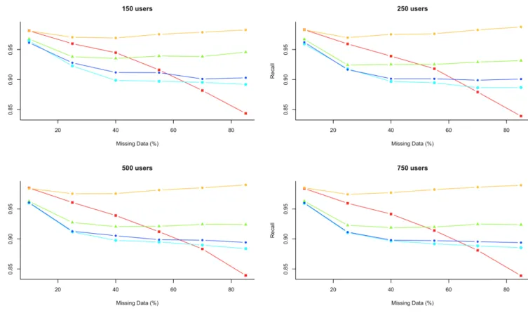
(38) In this specific metric, results do not have a variation depending of the size of the dataset. In all four cases, it can be seen that the number of recommended items increases with the increase of the percentage of missing data due to the existence of more items that the users haven’t seen and, thus, can be recommended. Note that, for this specific dataset, a threshold of 4 was set so the recommender system returned those items that were estimated to have a predicted rating above that value. It can be seen that when the percentage of missing data is low, below 30%, there’s no difference in the length of the recommendation lists. In the same way, in the case where the percentage of missing data is higher than 50%, the recommender system is able to generated a greater number of recommendations per user from the datasets which have been pretreated using imputation methods. 6.1.2. Recall, precision and F1-score. Since the final aim of a recommender system is to generate a set of good recommendations for each user, the chosen way to evaluate its performance has been the use of recall and precision metrics. Keeping in mind that recall express the percentage of relevant items that where recommended to the user out of all the unrated ones, the obtained results are as follows.. Figure 10: Poisson dataset recall results 29.

(39) Note that the Poisson dataset was created using a combination of Poisson distributions, which are based on a occurrence rate or mean, in order to generate the ratings of the 15 items and, as previously seen, most of the items share a similar mean value. Furthermore, 4 well defined groups of users can be distinguished. As a consequence of these facts, high values of recall, from 85% and up to 99% have been obtained. A common pattern can be seen in the obtained recall scores regardless of the number of users. On the one hand, the recall score of the recommender without any previous treatment of the data, decreases exponentially as the percentage of missing data increases. It can also be seen that when there is a 40% or a greater value of missing data, some imputation methods obtain a better recall score than the usual recommender method. On the other hand, in the case of the application of imputation methods, even thought in general there is a decrease of its performance, when the percentage of missing values overcomes 40%, there is an stabilization of the recall score. The Mean Substitution method obtains an unbeatable performance in terms of recall. As mentioned previously, this is tightly associated with the algorithm used to generate the ratings. Between the applied hot-deck method and the Proposed method, which is also a variant of a hot-deck method, the first one obtains a better performance. In this case, as there isn’t a scale variation problem because all the ratings share the same scale and there isn’t outliers, the proposed method is not likely to make a significant improvement from other Hot-deck methods. Finally, the imputation method that has a worse performance is the PMM-based Multiple Imputation, it’s not a surprising fact given the almost inexistent linear relationships between the items. The other accuracy metric that has been considered is precision. It measures the number of recommended items that are relevant, that is, those that really have a rating above 4.. 30.

(40) Figure 11: Poisson dataset precision results The first interesting thing that can be seen in the obtained results, is the turn back of the imputation methods performance. In terms of precision, the PMM-based MI method it the one that gets the best score regardless of the number of users. Thus, at the same time, the Mean Substitution method is the one that obtains a worse score. What can be extracted from this fact is that even if the PMM-MI method leaves a greater number of relevant items without recommendations, it is more accurate in its recommendation generation, having a higher percentage of items that the user is really going to like. With the Mean Substitution happens exactly the other way around, it is not as exact with its recommendations, it can recommend items that the user will not like, but it has a higher probability to recommend a larger number of relevant items. In this case, the hot-deck methods make the recommender have an alike performance in terms of precision that the one without doing an imputation of the data. It can also be seen the influence of the missing data in the results, leading to a decrease of the precision results when it increases its volume into the data, although with greater percentage than 30%, a stabilization can also be seen.. 31.

(41) Figure 12: Poisson dataset F1-score results Finally, one can use F1-score to represents the harmonic mean of Precision and Recall, obtaining a unique measure of the performance. This test dataset has highlighted the fact that just precision or recall by their own are not enough descriptive in order to check the accuracy performance of a recommender system and, thus, an analysis of what is more important in our specific context should be made in order to choose the imputation method. In spite of that fact, it’s clear that the use of imputation methods can improve the accuracy of recommender systems. 6.1.3. Execution Time. Finally, the computational cost of the imputation methods has also been considered, specially in the case of real time recommender, where a good performance in terms of time is required. In Figure 13, one can find the obtained times of the imputation methods in the Poisson dataset.. 32.

(42) Figure 13: Poisson dataset execution time results As it can be seen, the size of the dataset matters when it comes to execution times. A greater number of users will directly mean a time increase. This is specially true for the proposed imputation method. The noticeable difference with the other methods is due to the computation of the variance-covariance matrix for each user. As it does not vary regardless of the recipient chosen, it can be stored in memory and accessed whenever is required in order to decrease the execution time required. This solution has not been applied in this thesis because we aimed to an equitable comparison between the methods, as the others had not been treated in any special way. It can also be seen that the Multiple Imputation method also consumes a larger time. This fact is due to the several times that the method has to do an imputation method plus the time it takes to analyze the obtained results and mix them into the final estimated values for each missing rating.. 33.