INSTITUTO TECNOLÓGICO Y DE ESTUDIOS SUPERIORES DE MONTERREY
PRESENTE.-Por medio de la presente hago constar que soy autor y titular de la obra denominada
, en los sucesivo LA OBRA, en virtud de lo cual autorizo a el Instituto Tecnológico y de Estudios Superiores de Monterrey (EL INSTITUTO) para que efectúe la divulgación, publicación, comunicación pública, distribución, distribución pública y reproducción, así como la digitalización de la misma, con fines académicos o propios al objeto de EL INSTITUTO, dentro del círculo de la comunidad del Tecnológico de Monterrey.
El Instituto se compromete a respetar en todo momento mi autoría y a otorgarme el crédito correspondiente en todas las actividades mencionadas anteriormente de la obra.
De la misma manera, manifiesto que el contenido académico, literario, la edición y en general cualquier parte de LA OBRA son de mi entera responsabilidad, por lo que deslindo a EL INSTITUTO por cualquier violación a los derechos de autor y/o propiedad intelectual y/o cualquier responsabilidad relacionada con la OBRA que cometa el suscrito frente a terceros.
CAN-based Network System for Speed Control of an
Autonomous Vehicle-Edición Única
Title CAN-based Network System for Speed Control of an Autonomous Vehicle-Edición Única
Authors Jesús Alfredo del Bosque Garza
Affiliation Tecnológico de Monterrey, Campus Monterrey
Issue Date 2010-12-01
Item type Tesis
Rights Open Access
Downloaded 18-Jan-2017 19:11:43
Instituto Tecnológico y de Estudios Superiores de
Monterrey
Campus Monterrey
School of Engineering
Division of Mechatronics and Information Technologies Graduate Programs
Master of Science Major in Intelligent Systems
Thesis
CAN-based Network System for Speed Control of an
Autonomous Vehicle
by
Jesús Alfredo Del Bosque Garza 786850
CAN-based Network System for Speed Control of an
Autonomous Vehicle
By
Jesús Alfredo Del Bosque Garza
Thesis
Presented to the Graduate Program in Information Technologies and Electronics at the
Instituto Tecnológico y de Estudios Superiores de Monterrey as partial fulfillment of the requirements for the degree of
Master of Science
major in
Intelligent Systems
Campus Monterrey School of Engineering
Division of Mechatronics and Information Technologies Graduate Programs
The committee members, hereby, recommend that the thesis presented by Jesús Alfredo Del Bosque Garza be accepted as a partial fulfillment of the requirements to
be admitted to the degree of Master of Science, major in:
Dr. Ramon F . Brena Pinero
Director of Master of Science in Intelligent Systems Division of Mechatronics and Information Technologies
VII
Table of Contents
1 Introduction ... 1
2 Methodology ... 9
2.1 Analysis and Characterization ... 11
2.1.1 Utilitarian Electric Vehicle ... 11
2.1.2 Ackerman Steering Mechanism ... 12
2.1.3 Kinematic Model ... 13
2.1.4 Motor Model ... 14
2.1.5 Electric Model ... 15
2.1.6 Millipak Controller ... 18
2.1.7 Network Controlled System ... 19
2.1.8 Controller Area Network ... 21
2.1.9 Programmable Automation Controller ... 34
2.2 Design ... 36
2.3 Implementation ... 39
2.4 Testing... 43
2.4.1 Repeatability Test ... 45
2.5 Corrections and Modifications ... 49
3 Implementation ... 51
3.1 Wheel Speed Sensor ... 51
3.2 Modules and Interfaces ... 53
3.2.1 SPI-CAN Module ... 53
3.2.2 MCU Module ... 55
3.2.3 Millipak Interface ... 57
3.3 CAN Nodes Description ... 60
3.3.1 Millipak CAN Node ... 60
3.3.2 Wheel Speed Sensor CAN Node ... 61
3.3.3 CompactRIO CAN Node ... 62
3.3.4 Node Mounting ... 62
3.4 CompactRIO ... 64
3.4.1 LabVIEW Project Configuration ... 64
3.5 Timing ... 66
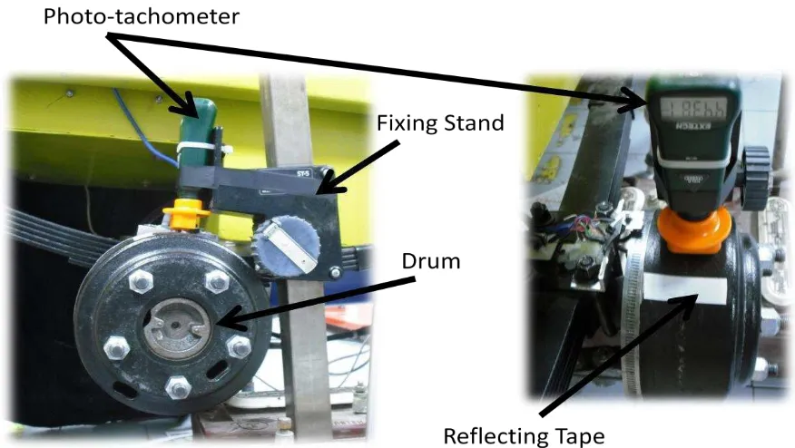
3.6 RPM Measurement ... 66
3.7 Process Characterization ... 73
3.8 PID Control ... 74
3.8.1 PID Tuning ... 76
3.9 Fuzzy Logic Control ... 77
3.9.1 Fuzzy Logic System ... 78
4 Experiments and Results ... 83
4.1 CompactRIO PID Control ... 83
4.2 CompactRIO Fuzzy Logic Control ... 85
5 Conclusions ... 87
Appendix A Kinematic Model ... 91
Appendix BMotor Model ... 95
Appendix CMillipak Controller ... 97
Appendix DWheel Speed Sensor... 103
IX
Figure List
Figure 1-1: Main elements of the control architecture for an AV as proposed by
Albores in [Albores, 2007]. ... 5
Figure 1-2: CAN control architecture for an AUV presented by [Zhao et al., 2010]. .... 6
Figure 2-1: Research development methodology. ... 9
Figure 2-2: The Johnson Industries Super Truck testing platform. ... 11
Figure 2-3: General layout of the vehicles mechanical composition. ... 12
Figure 2-4: The ICR created by the Ackerman mechanism. ... 13
Figure 2-5: Vehicles posture definition. ... 13
Figure 2-6: Equivalent circuit for the separately excited DC motor. ... 14
Figure 2-7: General representation of the main electric circuits of the vehicle. ... 15
Figure 2-8: Control circuit.. ... 16
Figure 2-9: Auxiliaries circuit.. ... 17
Figure 2-10: Electric motor circuit. ... 17
Figure 2-11: General representation of a Network Control System with induced delays on the sensor and controller. ... 21
Figure 2-12: Devices, modules and electronic control units without a CAN bus implementation require considerably more wiring in a system (left). ... 22
Figure 2-13: Different networks inside a common vehicle. ... 22
Figure 2-14: CAN bus representation in BMWs R1200 and K1200 motorcycles. ... 23
Figure 2-15: Domo’s CAN bus node architecture. ... 24
Figure 2-16: Transfer rate versus bus length for CAN bus over a twisted pair wire medium. ... 25
Figure 2-17: Transmission lines CAN High and CAN Low with bus termination resistors. ... 26
Figure 2-18: Logical levels over CAN bus. ... 26
Figure 2-19: OSI reference model. ... 28
Figure 2-20: Nominal bit time segments as defined by Microchip. ... 29
Figure 2-21: Nominal bit time segments defined by Philips. ... 29
Figure 2-22: Standard message frame format for the CAN protocol. ... 30
Figure 2-23: Extended message frame format for the CAN protocol. ... 30
Figure 2-25: Structure of the cRIO embedded system. ... 35
Figure 2-26: Typical architecture for an embedded system using CompactRIO. ... 36
Figure 2-27: CAN Node basic structure. ... 37
Figure 2-28: Two different but equivalent implementations evaluated for the CAN modules. ... 37
Figure 2-29: CAN nodes physical distribution along the vehicle. ... 40
Figure 2-30: Conceptualization for the CAN-based NCS implemented. ... 42
Figure 2-31: Testing conditions for the vehicle... 43
Figure 2-32: Schematic of the developed CAN bus. ... 45
Figure 2-33: Repeatability test setup. ... 46
Figure 2-34: RPMs versus sample number are shown as results of the 50% of max speed test. ... 47
Figure 2-35: RPMs versus sample number are shown as results of the 100% of max speed test. ... 47
Figure 2-36: a) Slightly affected signal quality. b) Undesired impulses between pulse signals generated during the operation of the vehicle. ... 50
Figure 2-37: Signal quality improvement from the usage of twisted pair wire. ... 50
Figure 3-1: ITR8102 opto-interrupters used for the wheel speed sensor. ... 52
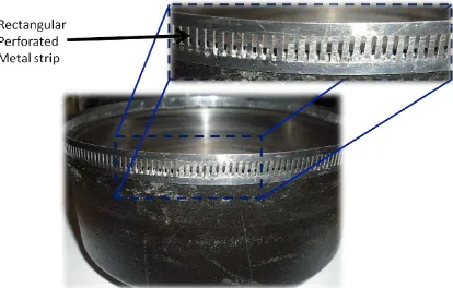
Figure 3-2: Third version of the wheel speed sensor, using the rectangular perforated metal strip. ... 52
Figure 3-3: SPI-CAN module electric schematic. ... 54
Figure 3-4: SPI-CAN module PCB schematic. ... 54
Figure 3-5: SPI-CAN module. ... 55
Figure 3-6: MCU module electric schematic. ... 56
Figure 3-7: MCU module PCB schematic. ... 56
Figure 3-8: MCU module. ... 57
Figure 3-9: Millipak interface electric schematic. ... 58
Figure 3-10: Millipak interface PCB schematic. ... 58
Figure 3-11: Millipak interface. ... 58
Figure 3-12: Wheel speed sensor interface electric schematic. ... 59
Figure 3-13: Wheel speed sensor interface PCB schematic... 59
Figure 3-14: Wheel speed sensor interface. ... 60
Figure 3-15: Millipak node mounting and main CAN bus line. ... 63
Figure 3-16: Wheel speed sensor node mounting showing Millipak controller. ... 63
Figure 3-17: Top view of both nodes on the vehicles back part. ... 64
Figure 3-18: Programming levels of a cRIO project. ... 65
Figure 3-20: Plots from top to bottom; the period method, the pulse count method, mode filtered pulse count method, median filtered pulse count method and median filtered period method. ... 69 Figure 3-21: Close-up on the constant speed section of figure 3-20. Again, plots from
top to bottom; the period method, the pulse count method, mode filtered pulse count method, median filtered pulse count method and median filtered period method. ... 70 Figure 3-22: Delayed signal induced by the application of the median filter on the
pulse count method measurement. ... 71 Figure 3-23: Delayed signal induced by the application of the median filter on the
period method measurement. ... 71 Figure 3-24: Systems response to a 100% change in speed demand. From top to
bottom, median filtered pulse count method, pulse count method and period method. ... 72 Figure 3-25: The systems response curve used for characterization. Each sample
marked on the horizontal axis corresponds to a 30 millisecond interval. 73 Figure 3-26: Block diagram of a typical NCS with induced delays. ... 75 Figure 3-27: Membership function for the input variable Error. Error units are in
RPMs. An error bigger than 28 RPMs (either positive or negative) represents a large error. The zero error range is defined in conjunction with the Positive and Negative error range, membership varies depending on the three different linguistic terms. ... 79 Figure 3-28: Membership function for the input variable Error Change Rate. Error
units are in RPMs. As with the other input variable, 5 terms are used to describe the state of the error change rate variable. ... 80 Figure 3-29: Membership function for the output variable CAN Data Changes. ... 80 Figure 3-30: Fuzzy Space described by the rule base. ... 81 Figure 4-1: Closed Control Loop response with PID controller. Showing sample time
(each time sample is equal to 50 milliseconds) on the horizontal axis versus percentage of maximum on the vertical axis. ... 84 Figure 4-2: Closed Control Loop response for setpoint change with PID controller
after Z-N tuning. ... 84 Figure 4-3: Closed Control Loop response for setpoint change with PID controller
after fine tuning the Z-N method. ... 85 Figure 4-4: Closed-loop response with fuzzy logic controller. ... 86 Figure 4-5: Closed-loop response with fuzzy logic for setpoint change. On the upper
XIII
Table List
Table 2-1: Standard specifications for the Millipak electric controller. ... 18
Table 2-2: Preset 7 description. ... 19
Table 2-3: I/O configuration for the Millipak. ... 19
Table 2-4: Analog functions for the Millipak ... 19
Table 2-5: High Speed CAN cable requirements. ... 41
Table 2-6: Results for the left wheel ... 48
Table 2-7: Results for the right wheel ... 48
Table 3-1: Message structure accepted by the Millipak CAN node. ... 60
Table 3-2: Message structure broadcasted by the sensor CAN node. ... 61
Table 3-3: Process parameters: dead time , time constant and . ... 74
Table 3-4: PID tuning parameters. ... 76
Table 3-5: ITAE tuning parameters calculated. ... 76
Table 3-6: Ultimate gain PID tuning parameters. ... 77
Table 3-7: Relationship between error, error change rate, and process variable. ... 79
XV
Abstract
The work hereby presented deals with the partial automation of a utilitarian ground electric vehicle; in particular with the development and implementation of a Network Control System (NCS) using a Controller Area Network (CAN) based bus for speed control. This thesis highlights the use and development of standardized components and protocols in order to provide an easily upgradeable platform for future work, with enough robustness, reliability, and efficiency.
A Programmable Automation Controller (PAC) is used to develop and execute the speed control algorithm, and eventually can act as a human-machine interface via a personal computer. The kinematics involved are those of a rear-wheel differential driven conventional vehicle. An electric power controller is used to manage current and voltage flowing to/from the separately excited electric motor driving the vehicle. To develop the Network Control System based on the CAN protocol, CAN modules and additional specialized interfaces were manufactured, as well as CAN compliant cables and CAN hubs. A wheel speed sensor which functions as an incremental optical encoder was manually assembled in the Robotics Laboratory at the Tecnologico de Monterrey (ITESM). The CAN network is fully operational and has been tested proving to be a reliable channel for critical control information. The speed control algorithm is based on the proportional–integral–derivative (PID) controller model; tuning parameters were calculated and fine tuned via trial and error testing. Also, a fuzzy logic controller was developed to compare its performance against that of the PID.
1
Chapter 1
1
Introduction
Demand for robotic applications has increased in areas that range from exploration to entertainment [Guo, 2008]. The development of mobile robots on the educational, private and military sectors has driven focus for research; modern trends indicate the use of robotic applications for working environments in which the tasks involved are dirty, dull or dangerous [Braybrook, 2004; Álvarez et al., 2006] for operators, making necessary the automation of functions previously done by humans. The development of autonomous mobile robots has demonstrated to be a challenging topic in the fields of computer science, electrical and mechanical engineering.
Automation deals with the detachment of robots from their human operators. Decisional autonomy in robotics is intended to reduce the number of remote operators, change their roles and decrease their workload [Barbier et al., 2009]. During the automation process, an early and crucial stage is the selection and installation of communication channels, sensors and actuators (instrumentation1) which will later provide the means for the robot to interact with its surrounding environment.
Autonomous vehicles (AXV2 or AV) are a type of autonomous mobile robots3 that have gathered significant attention due to characteristics such as precision,
1According to the International Society of Automation (ISA) the official definition for instrumentation
(ISA standard S51.1) is: A collection of instruments or their application for the purpose of observation, measurement, control, or any combination of these [ISA, 1992].
2X
denotes medium for navigation, e.g. AGV: Autonomous Ground Vehicle; AAV: Autonomous Aerial Vehicle; AUV: Autonomous Underwater Vehicle; ASV Autonomous Surface Vehicle [Barbier et al., 2009].
3 A distinction is made between these concepts. The term autonomous vehicle usually means the
repeatability, speed, and most of all, the ability to perform specialized tasks on hazardous environments, where human integrity might be at risk.
A common practice to develop an AV is the instrumentation and automation of utilitarian vehicles, where special care should be taken during the design and implementation of the underlying core information systems of the AV. Reliable protocols and components should be applied to ensure proper and successful operation. Furthermore, as technological advance continues to grow exponentially, to extend the lifespan of applied solutions, widely accepted standardized elements should be employed.
According to DARPA4 “An autonomous ground vehicle is a vehicle that navigates and drives entirely on its own with no human driver and no remote control. Through the use of various sensors and positioning systems, the vehicle determines all the characteristics of its environment required to enable it to carry out the task it has
been assigned”.
Over the last two decades one of the main topics of the scientific community, dealing with human-robot interaction environments, has been the relief of disaster scenarios. International associations such as the Institute of Electrical and Electronics Engineers (IEEE) have developed specific research divisions for this area. The term rescue robotics involves systems that are designed to support human first response units during dynamic disaster situations. Applications for rescue robotics include: information gathering of the disaster; hazardous material handling; search, diagnosis and rescue of survivors; quantitative investigation of the damage extent; support for recovery actions and help at evacuation centers [Tadokoro, 2009]; leaving people with the ability to concentrate on high priority actions.
The rescue robotics area requires autonomous vehicles capable of withstanding harsh environmental conditions. High quality standardized components that are able to operate during vibrations, in hot or cold environments, with high electromagnetical noise, humidity, etc., along with complementary software, such as standard communication and navigation protocols, must be used to prototype the AVs acting on these environmental conditions.
Controller Area Network (CAN) is a serial communication protocol that can be used for real-time distributed control. This bus architecture has proven to be a
4DARPA is the Defense Advanced Research Projects Agency created in 1958 by the United States of
confident medium for modular configurations. With CAN bus, it is possible to implement a Network Controlled System (NCS) or field bus [Davis, 2010] for closed-loop control with relatively low cost and high efficiency. Advantages like less wiring, modularity and interoperability arise from the adoption of this technology.
The automation process can yield as a result functional but complex control architectures. Attempts at the development of an AV, without the application of standardized components and protocols, often result in customized solutions, where only the developers are able to fully understand the know-how involved.
The communication protocol used not only defines software constraints; hardware considerations, like cable types, cable length and network topology, are also dependable on protocol selection. Complex architectures usually require complex data pathways (physical connections), making wiring inside the vehicle a major concern. Maintenance and replacement of customized components, as well as inclusion of new elements may result in a challenging task. The lack of consideration for upgrading capabilities makes these solutions prone to obsolescence.
Therefore, an issue arises during the early development of an AV. When selection
of the components for the system’s architecture is not based on standards; compatibility, interoperability, robustness, reliability and quality can’t be assured; compromising future implementations.
The use of standard certified elements guarantees a general understanding of the applied technology, providing a strong, reliable and common groundwork while maintaining important know-how information for further development and simplifying implementation, maintenance, upgrading times and costs of the system.
The work presented here addresses to prove that a Network Control System based on the CAN standard specification is reliable and robust enough for the development of the control architecture of an autonomous ground vehicle. Using standardized components and protocols that provide minimum cost and a relatively easy implementation, a full control loop can be established.
In particular the objectives in this research are:
1. Development and implementation of a CAN network for the vehicle. 2. Development of modular CAN interfaces.
3. Subdivision and organization of the system into a distributed network composed of different CAN nodes.
4. Development of a closed-loop NCS with expanding capabilities.
5. Development of a programming solution for the speed control module of the system architecture using a PAC.
6. Establishment of a common ground for future development.
The functions performed by the vehicle constitute different abstractions within the systems architecture; a basic structure contains methods for environmental perception, action planning and control. While these are all tasks performed by humans during a vehicles standard operation, other no so evident functions have to be performed as well. Figure 1-1 shows the basic elements in an AV architecture, where the speed control module is highlighted inside the red square. The complete architecture is composed of different modules, where their interactions are described by information sharing communication channels.
Movement of the vehicle can be traced on a 2-D plane, where localization at any given time can be described by its coordinates and its orientation . Control is performed in the vehicles trajectory5 in function of its steering angle and its velocity6 .
The vehicle used during this research can be modeled beside its Ackerman steering mechanism. Velocity control is crucial for overall operation and efficiency as it plays a major role inside the kinematic model of the vehicle, typically used with dead reckoning techniques for pose estimation and steering control [Borenstein, 1994]. Being the base for speed estimation, the velocity control module constitutes a fundamental element inside the AVs architecture.
5 A trajectory is defined as an ordered collection of points, composed by positions and orientations
[Albores, 2007].
6
Figure 1-1: Main elements of the control architecture for an AV as proposed by Albores in [Albores, 2007].
Although this thesis deals with speed, it is simple to measure velocity once its magnitude is known, since only direction of the moving vehicle is needed.
The standardized CAN protocol makes possible the integration of information managed by the real-time network with the high computational power of a Programmable Automation Controller (PAC), which offers the industrial ruggedness of a specialized Programmable Logic Controller (PLC) combined with the versatility of a Personal Computer (PC).
Figure 1-2: CAN control architecture for an AUV presented by [Zhao et al., 2010]. The scope of this thesis covers the implementation of the CAN communication network inside the vehicle for integration of the modules composing the system’s
architecture. While the complete architecture is integrated by different modules, in this research only the speed control module is developed.
The main contribution achieved is the establishment of a complete closed control loop, composed by three different CAN nodes.
This thesis is divided in 5 chapters and several appendices. Below is brief description of such chapters.
Chapter 2 presents the methodology followed for the successful development and implementation of a Network Control System based on the CAN protocol for speed control of the utilitarian electric vehicle, used in this thesis. A description of the elements in such methodology is presented.
Chapter 3 presents the implementation of the key elements developed for this project. This chapter extends the details of elements generally presented on chapter 2.
Finally, Chapter 5 shows the conclusions of this work. Evaluation of the elements developed is presented as well as possible improvements and implementations for future work.
9
Chapter 2
2
Methodology
The methodology followed is shown in figure 2-1, it is similar to the one presented by Gonzalez in [Gonzalez, 2004]. Some of the steps involved were done separately for the implementation of the CAN network and for the speed controller. This entire research was done with aid from members of the E-Robots research group from the Robotics Laboratory at Tecnologico de Monterrey.
Analysis and Characterization:
A breakdown of the mechanical and electric systems composing the vehicle is made. Documentation provided by different manufacturers is thoroughly examined to fully understand the elements involved and their limitations. Characterization of the vehicle is done; different models are constructed, for instance the electric model, consisting of the schematic diagram of the electric wiring configuration; and the mechanical model, including the kinematic model of the vehicle and the dynamical model of the motor driving the vehicle.
In a similar manner, research is done concerning network controlled systems in order to understand their structure and characteristics. The CAN protocol is revised to understand its performance, restrictions and standard specifications.
Design:
Hardware and software solutions for new systems or modifications to existing ones are designed during this phase. At this point, selection of the necessary elements to implement a network based on the CAN protocol for closed loop speed control takes place.
Simple experimental testing is done on these designs in order to avoid malfunctioning during the implementation phase.
Implementation:
During the implementation phase, all designs conceived and tested on the previous stage are developed. Manufacturing of the necessary components for automation, modifications required on existing elements, as well as software programming is done. The complete NCS is assembled. After this phase the first prototype emerges and is ready for testing.
Testing:
The goal of this stage is to measure the performance obtained by the designed implementation and improve it through several corrections on the system.
Corrections and Modifications:
Corrections and modifications help with the improvement of the control system; depending on the magnitude of such actions, the methodology can be reset to the design, implementation or testing phases. Once all tests prove successful, a prototype vehicle with autonomous speed control emerges.
2.1
Analysis and Characterization
2.1.1
Utilitarian Electric Vehicle
The vehicle used for this research is characterized with non-holonomic constraints due to its Ackerman steering mechanism; this means that rolling exists without lateral slipping between the wheels and the ground [Habumuremyi, 2005]. Non-holonomic constraints restrain the vehicle from moving instantaneously in any direction; they involve a higher number of effective degrees of freedom (DOF) than controllable ones. In order to change orientation, the wheels need to change direction and the vehicle has to move either forward or backward. The maneuverability of the vehicle is described by the degree of mobility , which deals with the degrees of freedom that can be manipulated for the vehicles motion; and the degree of steeribility , which deals with the number of centered orientable wheels that can be steered independently to steer the vehicle. The degree of maneuverability , is the overall degrees of freedom that the vehicle can effectively manipulate, which is simply the sum of the mobility and steeribility measures [Xiao, 2008; Campion et al., 1996]. For the case of an Ackerman steered vehicle the degree of mobility is 1 and the degree of steeribility is also 1 (making the degree of maneuverability,
), this is why car-like vehicles are said to have 2 effective DOF.
The utilitarian vehicle employed is the Super Truck model from Johnson Industries, originally designed to work on mining environments. It is shown in figure 2-2.
Some characteristics of the Super Truck include: • 1600 lb payload.
• 17 mph maximum speed (14 mph loaded). • 5Hp motor.
• 11 gauge steel body.
• 600 ampere Solid State Controller. • Six deep cycle battery, 36-volt system.
The vehicle follows a mid-engine rear-wheel drive layout; with a differential on the motors output shaft for torque transmission between the rear driving wheels, as shown in figure 2-3.
Figure 2-3: General layout of the vehicles mechanical composition. [Habumuremyi, 2005]
2.1.2
Ackerman Steering Mechanism
Figure 2-4: The ICR created by the Ackerman mechanism.
2.1.3
Kinematic Model
For an base frame, the mobile platform system can be defined as with its origin at the middle of the vehicle’s rear axis. The vehicles orientation is measured with respect to . Position and orientation may be described at any time by: . A simplified bicycle model assumes one mobile centered wheel with an angle measured with respect to , that is typically taken as the average between the orientation angles of each of the two steering wheels.
Figure 2-5: Vehicles posture definition.
the control architecture, since velocity affects proportionally the kinematic model, thus affecting position estimation. Detail on the kinematic model is presented in Appendix A.
(2.1)
2.1.4
Motor Model
The vehicle has a 5HP, 36 volt separately excited direct current electric motor as the main driving mechanism. An electric motor takes energy as an input and produces torque (or speed, depending on its operating curve) as an output. Speed and torque depend on the voltage applied on the motor and the current it draws. In a separately excited DC motor, the field current is supplied by a constant voltage supply; the field winding excites the field flux while the rotor’s brushes and
commutator supply the armature current. When a separately excited motor is excited by a field current and an armature current is flowing in the circuit, a back electromagnetic field and a torque are developed at a particular speed [Salam, 2003]. Figure 2-6 shows the separately excited motor’s equivalent circuit.
Figure 2-6: Equivalent circuit for the separately excited DC motor. [Salam, 2003] Detail on the dynamical model for obtaining the motor’s transfer function is presented in Appendix B. The transfer function for the electric motor is:
The motor model describes a first order system. A proportional-integral-derivative controller is suitable to control this type of systems without much complexity; hence the selection of such control algorithm for the physical system is theoretically validated by the model.
2.1.5
Electric Model
To understand how the electric vehicle works, the electric diagram representing its circuitry was constructed. This electrical model shows the connections between the different electric elements inside the vehicle.
Special interest is taken on the power controller installed on the vehicle. The Millipak controller manufactured by Sevcon, functions as a power interface between the control lines and the motor. A general representation of the main elements in the circuit is shown in figure 2-7.
Figure 2-7: General representation of the main electric circuits of the vehicle. The vehicle’s electric circuit can be classified in three distinctive parts; the main or
The control circuit occupies the major part of the vehicle’s wiring. The accelerator signal, fail safe switch in the accelerator pedal and functions located on the manual control panel like the on/off key switching of the system, lights operation, displacement direction selection (forward/reverse) and emergency stop are part of the control circuit.
The auxiliaries’ circuit connects secondary elements that are not necessary to drive the vehicle; these include the horn, the battery charge meter and the control
mechanism in charge of lowering and raising the vehicle’s cargo bed. Devices on this circuit are not interrupted when the emergency stop is pressed.
The connections between the 5HP driving motor and the Millipak power controller are fairly simple. The Millipak controller internally regulates the current and voltage
applied to the motor’s terminals according to control signals sent through connector
B (shown in figure 2-8).
Figure 2-8: Control circuit. Elements contained in the front control panel and accelerator pedal are shown inside the dashed lines. The relay connects the positive terminal of the Millipak controller to the batteries once the key has been switched to
Figure 2-9: Auxiliaries circuit. Elements in the auxiliaries’ circuit are not required to
drive the vehicle. The horn, battery meter and the motor for the vehicle’s cargo bed are independent of the elements in the other circuits.
Figure 2-10: Electric motor circuit. The batteries positive and negative terminals are connected to the respective B terminals of the Millipak controller. Within the figure
2.1.6
Millipak Controller
The Millipak controller from Sevcon regulates the power administered to the separately exited electric motor (SEM) on board the Super Truck. All the information presented in this section was taken from [Sevcon, 2004] and through contact with technical assistants at Sevcon. Some of the characteristics of the controller are shown in table 2-1:
Table 2-1: Standard specifications for the Millipak electric controller.
Characteristic Rating Battery voltage 24/48 VDC Peak current 500 A / 600 A Continuous current 180 A /200 A
Field current 40 A
Max. power 6.5 kW
Operating temperature -30 to + 40ºC Storage temperature -40 to + 70ºC Ingress of dust and water IP66
Humidity 95% (at 60ºC)
Vibration 6G
Switching frequency 16 kHz
Two types of connectors are located on the Millipak. First, connector A, for diagnosis and programming via a proprietary tool from Sevcon, denominated
“calibrator”. Second, connector B, where control signals are received in order to drive the electric motor. Refer to Appendix C for details.
The digital inputs, analogue inputs and contactor drive outputs available on connector B can be configured in a number of ways to suit various applications. Different presets are preprogrammed by Sevcon. To operate the controller one of these presets has to be selected. Once a preset has been selected the pins on connector B are allocated according to the preset’s definition and a list of parameters or personalities defining certain characteristics on the controller become available for user modification.
Table 2-2: Preset 7 description.
Digital
Function Description
7 Ride On vehicle with Speed Cutback 1 and 2 switches and external LED drive.
Table 2-3: I/O configuration for the Millipak.
Digital Function 7
Forward B2
Reverse B3
FS1 B4
Seat B5
Speed Cutback 1 B6 Speed Cutback 2 Bw Line Contactor B8 External LED B9
Bw refers to pin B11, which can be used as a digital input if analog input 2 is configured as a digital input also. Analog functions are presented in table 2-4; analog input configuration 3 was used, leaving B10 as the accelerator input and B11 as a digital input.
Table 2-4: Analog functions for the Millipak
Analog Function 3 Accelerator B10
Digital B11 Footbrake
The calibrator tool was used for the system’s in-depth analysis and personal configuration. Refer to Appendix C for details on the Millipak configuration information.
2.1.7
Network Controlled System
network. This type of setup offers several advantages over traditional point-to-point control solutions, some which are: modularity and flexibility for system design; simple and fast implementation; ease of system diagnosis and maintenance; decentralized control and increased system agility. These advantages are translated into characteristics such as distributed processing, interoperability, reduced wiring, small power requirements and complexity of the physical connections, as well as the possibility of information exchange between different control loops; all which ultimately represent a reduction in costs [Huo et al., 2004; Chow & Tipsuwan, 2001]. In a NCS, sensors and actuators are connected directly to the desired plant and also to the real-time network. The controller, while physically separated from the plant, is also connected to the real-time network, closing the control loop [Lihua et al., 2008]. Proper interconnection of every device on the network depends on the protocol being used. A general representation of the elements included in a NCS is shown in figure 2-11.
Systems controlled by an NCS can be modeled as “discrete-continuous” with time
varying elements induced by the network. These induced delays depend on different factors, like network type, cable lengths, and baud rates used. The medium access method affects time variations since every device (referred as a node) competes for broadcasting time on the network, where collisions are meant to happen. Collision handling is an important aspect that depends on the protocol used. Thus there exists a trade-off between the finite bus capacity and the performance of the control loop.
Figure 2-11: General representation of a Network Control System with induced delays on the sensor and controller. While sensor and actuator are directly attached
to the process plant the controller is physically separated but still connected to the other elements through the network.
2.1.8
Controller Area Network
Data management and communication systems play an important role within the vehicle’s architecture. A reliable communication system improves reaction times and minimizes uncertainty. Controller Area Network (CAN) is a vehicle bus standard for distributed environments originally designed by Robert Bosch [Bosch, 1991] to provide robust serial communication for a vehicle’s on board network. The CAN bus protocol offers standard network technology, with high error checking features. Some of the main features of CAN include the ability to use decentralized pre-processing by the inclusion of a microcontroller, which results in less computational work for higher level units. CAN is a broadcast serial bus, based on message exchange between different nodes.
Figure 2-12: Devices, modules and electronic control units without a CAN bus implementation require considerably more wiring in a system (left) [NI, 2009a]. In modern day vehicles several different networks interact with CAN bus. Usually the CAN network controls all real-time critical functions, such as ABS and traction control. Local Interconnect Network (LIN) is used as a sub-bus of CAN, typically for non-safety related critical tasks. The Media Oriented System Transport (MOST), also acting as a sub-bus of CAN, is used to control automotive multimedia. All networks within the vehicle are controlled by a main control system, which also acts as a gateway for all networks to share data [Leen & Heffernan, 2002]. Figure 2-13 shows vehicle network integration, where CAN functions as the main or top network and two different sub-networks operate on less critical functions.
CAN bus technology has made its inclusion not only on automobiles but also in other means of transportation, like motorcycles. BMW uses CAN bus for communication between proprietary control modules on its R1200 and K1200 models. These control modules share a data network through the CAN bus. An example is the interconnection between the Engine management system, called BMS-K (BMW Motor-Steuerung mit Klopfregelung); the Central Chassis Electronics, called ZFE (Zentrale Fahrzeugelektronik) and the Instrument Panel (I-Cluster). Additional modules like the Anti-lock braking system called ABS, and the Alarm System called DWA (Diebstahl Warnanlage) also interact through the CAN bus. The ZFE controls the lights, heated accessories, horn, radio, accessory socket, and cruise control based on inputs from handlebar switches. Control inputs go directly to ZFE, and control outputs go from ZFE to individual components. The BMS-K inputs include the starter button, kill switch, sidestand switch, clutch switch, gear position indicator, and various engine sensors. Outputs control the starter, fuel pump, injectors, ignition coils, and warning lights. Finally, the I-Cluster displays information to the rider; it has only one physical input, the clock setting button, while the outputs are the various instruments and warning lights [Largiader, 2006]. Information is broadcasted to the network by each module, but only modules that require it will act upon it. The I-Cluster is a good example of a CAN control module, because it gets all of its information from other control modules through the CAN bus rather than receiving it directly as an input from sensors and switches. Because of this the I-Cluster panel can be removed and replaced without interrupting any other control module on the network. Figure 2-14 shows a schematic of the CAN network shared by the control modules on a BMW motorcycle.
Besides its application on vehicles, the CAN protocol has lately penetrated the field of robotics. CAN bus is popular as a real-time communication network for devices within humanoids. For example, the Rh-1, a 1.3m height 21 degrees of freedom humanoid robot uses CAN bus for communication between some of its electronic components [UC3M]. Toni, another humanoid that was constructed by the University of Freiburg [Behnke, 2006] to participate in the robotic soccer challenge RoboCup; uses CAN bus to establish communication between all of its onboard microcontrollers. Domo, a humanoid intended for research in manipulation by incorporating force sensing modules in its joints, uses CAN bus as a communication channel between different digital signal processing microcontrollers located all over its body and the higher level computational system [Edsinger & Weber, 2004].
Figure 2-15: Domo’s CAN bus node architecture [Edsinger & Weber, 2004]. CAN Bus Protocol Overview
Figure 2-16: Transfer rate versus bus length for CAN bus over a twisted pair wire medium [Azzeh, 2005].
CAN bus is based on the Open System Interconnection (OSI) model created by the International Standards Organization (ISO), meaning it follows a layered approach, which enables interoperability with products from different manufacturers. The CAN protocol implements the two lower layers of the OSI model; data link and physical layers [Pazul, 1999] described next.
Physical Layer
The Physical Layer is responsible for interconnection between nodes in the network; it handles the transmission of electrical impulses across the communication medium and deals with timing, encoding and synchronization of the soon to be transferred bit stream.
A bit signal on the bus line can take two possible representations: recessive, which only appears on the bus when the nodes send recessive bits; and dominant, sent only by one node to be heard on the bus. This means that a dominant bit sent by one node can overwrite recessive bits sent by other nodes. This feature is used for bus arbitration.
Figure 2-17: Transmission lines CAN High and CAN Low with bus termination resistors [Corrigan, 2008].
For the two-wire bus, the recessive bus state occurs when the CAN Low and CAN High lines are at the same potential (2.5V), and the dominant bus state occurs when there is a voltage difference of ± 1V (CAN L = 1.5V and CAN H = 3.5V). The CAN bus remains in the recessive state while it is idle [Richards, 2005]. Differentially driven signals provide an advantage when dealing with voltage spikes; if a spike is encountered both line conductors are equally affected, maintaining the voltage differential between both wires, providing a certain degree of noise immunity [Azzeh, 2005].
Figure 2-18: Logical levels over CAN bus [Richards, 2005].
Data Link Layer
This layer also performs Medium Access Control (MAC) to prevent conflicts when two different nodes try to access the network at the same time. It performs the data encapsulation/decapsulation, error detection and control, bit stuffing/destuffing and the serialization and serialization functions. The use of a MAC method is called bus arbitration. As a consequence of arbitration no bandwidth is wasted; there are methods that a designer can use to predict the longest possible delay before any message is delivered.
The CAN communication protocol uses a Carrier Sense Multiple Access/Collision Detection (CSMA/CD) MAC method. CSMA means that every node on the network must monitor the bus, and only transmit messages when no activity is found. During periods of no activity, every node has an equal opportunity to transmit a message. The Collision Detection portion means that if two nodes start transmitting at the same time, a collision will be detected and the proper corrective action will be taken [Pazul, 1999].
A nondestructive bitwise arbitration method is utilized; with this, even if collisions are detected, messages remain intact after arbitration is completed. Higher priority messages suffer no corruption or delay during the arbitration process. Non-destructive bitwise arbitration makes use of dominant and recessive logic states. The CAN protocol defines a logic bit 0 as dominant and a logic bit 1 as a recessive bit. As the name suggests, a dominant bit state will always win arbitration over a recessive bit state. Since the field used in the message arbitration process is the Message Identifier (ID), the lower its value the higher the priority of the message. A node also monitors the state of the bus while transmitting, to check if the logic state it is trying to send appears on the bus, if the node is transmitting a recessive bit and detects a dominant bit on the bus, it automatically stops transmission and receives the dominant message. After the dominant message has been received and the bus is once again idle, the node is able to try retransmission of its own message [Pazul, 1999].
Two standards have been developed by ISO, specifying a 5V differential voltage over the physical layer interface. These are [Pazul, 1999]:
• ISO-11898: CAN High Speed with bit rates between 125kbps and 1Mbps. • ISO-11519: CAN Low Speed with bit rates up to 125kbps.
Figure 2-19: OSI reference model [Richards, 2005]. Bit Timing
Bit rate is characterized as the number of bits transmitted over a certain period of time. The CAN protocol allows bit rate programming, as well as number and location of data samples in a bit period. Optimal selection of these parameters ensures message synchronization and proper error detection. To achieve synchronization all the nodes must have the same nominal bit time. Since no clock is encoded in the data stream, receiving nodes must recover the clock and synchronize it to the
transmitter’s clock [Microchip, 2007; Jöhnk & Dietmayer, 1997].
lengthened or shortened for resynchronization. The sampling point defines at which part of the nominal bit time, the signal will be sampled to determine the logical state of the current bit.
Depending on the manufacturer of the hardware used, the segments composing the nominal bit time can be named differently. For example, for Microchip the nominal bit time is composed of 4 segments, as shown in figure 2-20, while for Philips the nominal bit time is composed of 3 segments as depicted on figure 2-21. It is important to refer to the specific manual of the hardware involved for programming details when setting up the network.
Figure 2-20: Nominal bit time segments as defined by Microchip [Microchip, 2007].
Figure 2-21: Nominal bit time segments defined by Philips [Jöhnk & Dietmayer, 1997].
CAN Message Frame
error; and 4) Overload frames, generated by nodes that require more processing time for messages already received.
The CAN protocol defines two data frame formats, the standard format, also known as CAN 2.0A appearing in figure 2-21; and the extended format shown in figure 2-22 known as CAN 2.0B. The difference between formats resides in the number of bits used for the identifier field. CAN 2.0A uses 11 bit identifiers, while CAN 2.0B uses 29 bit identifiers [Pazul, 1999; Azzeh, 2005].
Figure 2-22: Standard message frame format for the CAN protocol [Pazul, 1999].
Figure 2-23: Extended message frame format for the CAN protocol [Pazul, 1999]. The fields for the CAN frame format are all described in [Bosch, 1991; Pazul, 1999; Azzeh, 2005] and are as follow:
• Arbitration Field: Containing an 11 bit message Identifier (ID) and the Remote Transmission Request (RTR) bit. A dominant RTR bit indicates that the message is a Data Frame. A recessive value indicates that the message is a Remote Transmission Request and therefore the frame is a Remote Frame. A Remote Frame is a request by one node for data from some other node on the bus. Remote Frames do not contain a Data Field. To accomplish an RTR, a Remote Frame is sent with the identifier of the required Data Frame.
• Control Field: Containing six bits; the Identifier Extension (IDE) bit distinguishes between the CAN 2.0A standard frame and the CAN 2.0B extended frame. Followed by the Reserved Bit Zero (RB0) bit, which is a reserved bit and is defined to be a dominant bit by the CAN protocol. The four
bit Data Length Code (DLC) indicates the number of bytes in the “Data Field”
that follows.
• Data Field: Containing from zero to eight bytes of data.
• Cyclic Redundancy Check (CRC) Field: Guarantees the frame’s integrity; contains a 15 bit cyclic redundancy check code and a recessive delimiter bit. • Acknowledge (ACK) Field: Consisting of two bits; the first is the Slot bit which
is transmitted as a recessive bit and is overwritten as a dominant bit by those receivers which have successfully received the message, regardless of whether the node processes or discards the data. The second bit is a recessive delimiter bit.
• End of Frame (EOF) Field: Consisting of seven recessive bits.
Following the end of a frame, the Intermission Frame Space (IFS) appears; consisting of three recessive bits. After the three bit intermission period the bus becomes available, and other nodes may begin transmission of their messages.
A message transmitted with an extended frame format is almost the same as one with a standard frame format. By using the IDE bit in dominant form, frames are transmitted in standard format, if the IDE bit is recessive; the CAN extended frame format is used instead. Standard format frames have higher priority than extended frame formats, but by using an extended format higher number of different message identifiers are possible [Pazul, 1999].
CAN Error Handling
able to transmit and receive messages, to complete shutdown (or bus-off state) based on the severity of the errors detected. This is called Fault Confinement. No faulty CAN node will be able to monopolize the network’s bandwidth because faults will be confined and faulty nodes will shut off before bringing the network down. Correct bandwidth use for critical system information is guaranteed by Fault Confinement.
Five conditions that yield an Error Frame exist; these are [Pazul, 1999]:
• CRC Error: The Cyclic Redundancy Check failed (CRC) and an error occurs, an Error Frame is generated. Since at least one node did not properly receive the message, it is resent after a proper intermission time.
• Acknowledge Error: The transmitting node checks if the Acknowledge Slot, sent as a recessive bit, contains a dominant bit, with this it would acknowledge that at least one node received the message correctly. If this bit is recessive, then no node received the message properly. An Error Frame is generated and the original message is resent after a proper intermission time.
• Form Error: If any node detects a dominant bit in any of the following four segments of the message: End of Frame, Intermission Frame Space, Acknowledge Delimiter or CRC Delimiter; a Form Error is generated. The original message is resent after a proper intermission time.
• Bit Error: If a transmitter node sends a dominant bit and detects a recessive bit, or vice versa, when monitoring the actual bus level and comparing it to the bit that it has just sent. In the case where the transmitter sends a recessive bit and a dominant bit is detected during the Arbitration Field or Acknowledge Slot, no Bit Error is generated because normal arbitration or acknowledgment is occurring. If a Bit Error is detected, an Error Frame is generated and the original message is resent after a proper intermission time.
Once an error has been detected it is broadcasted via the Error Frame. The erroneous message is aborted and as soon as arbitration allows it, it is retransmitted. Each node is in one of the three possible error states generated by the above conditions, which are shown in figure 2-24 and described as [Pazul, 1999; Azzeh, 2005]:
• Error-Active: In this state, the CAN node can actively take part on the bus communication; it can send an Active Error Flag, which consists of six consecutive dominant bits. With this the bit stuffing rule is violated and causes all other nodes to send an Error Flag, called the Error Echo Flag. A node is Error-Active when both the Transmit Error Counter (TEC) and the Receive Error Counter (REC) are below 128. Error-Active is the normal operational mode, allowing the node to transmit and receive without restrictions.
• Error-Passive: A node becomes Error-Passive when either the Transmit Error Counter or Receive Error Counter exceeds 127. Error-Passive nodes transmit Passive Error Flags, which consist of six recessive bits. If this node is the only transmitter on the bus, the passive error flag will violate the bit stuffing rule and the receiving node(s) will respond with Error Flags of their own depending on their own error state. If the Error-Passive node in question is not the only transmitter or is a receiver, then the Passive Error Flag will have no effect on the bus due to the recessive nature of the error flag.
• Bus-off: A node goes into the Bus-Off state when the Transmit Error Counter is greater than 255. In this mode the node cannot send nor receive messages, achieving Fault Containment.
2.1.9
Programmable Automation Controller
A Programmable Automation Controller (PAC) is a compact controller that combines the capabilities of a PC-based control system and a Programmable Logic Controller (PLC) into an open flexible architecture.
PLC users that required highly advanced applications began evaluating PC based solutions. The PC offered a graphical rich programming and user environment, and utilized commercial components like floating point processors and high speed I/O busses, such as PCI and Ethernet. However PC based applications were not designed for rugged environments, system crashes and rebooting, non-industrially hardened components and unfamiliar programming environments for operators proved to be a major challenge [NI, 2007]. This forced the development of products that combined the software capabilities of the PC and the reliability of the PLC. The resulting new controllers combined the best PLC features with the best PC features [NI, 2007]. PACs have evolved incorporating open standard interfaces, multi-domain functionality, modular architectures and modern software integration. [Resnick, 2003].
PACs employ a multi-domain property and are not limited to sequential logic solving. They rely on a single, multi-discipline, integrated development environment that uses common name and process tags as well as a common database for all functions. This integration opens up the possibility of using a single human-machine interface (HMI) for monitoring all functions. The multi-domain capability greatly diminishes total cost by reducing the time needed for design, programming and engineering, while also lowering installation, start-up, training, maintenance and spare parts costs [Iversen, 2008]. Key requirements for any PAC include: open, modular architectures and compliance with industrial standards that range from programming languages (such as the IEC 61131-3 standard) to communication, networking and interoperability, ranging from Ethernet and its variations, to XML (eXtensible Markup Language) and OPC, an open communication standard [Iversen, 2008].
The CompactRIO, an example of this type of technology is presented next. The CompactRIO Programmable Automation Controller, manufactured by National Instruments (NI), is described both in hardware and software structure.
CompactRIO
CompactRIO (cRIO) is a Programmable Automation Controller that combines an embedded real-time processor with a field-programmable gate array (FPGA) chip. The FPGA chip is integrated with a reconfigurable chassis that provides the user with the possibility of including swappable I/O modules with built-in signal conditioning for connection of sensors and actuators. A general representation of the cRIO platform is shown in figure 2-25. Modules are connected directly to the FPGA chip on the chassis, which in turn is connected to the real time processor via a high-speed bus following the Peripheral Component Interconnect (PCI) standard.
Figure 2-25: Structure of the cRIO embedded system [NI, 2009b].
Custom applications can be achieved using the graphical programming environment LabVIEW and software module add-ons LabVIEW FPGA and LabVIEW Real-Time for programming of the FPGA chip and real-time processor respectively.
Typical CompactRIO architectures include the following components:
• A reconfigurable input-output (RIO) FPGA core application for communication and control.
• A time-critical loop for floating-point control, signal processing, analysis, and point-by-point decision making.
• Normal-priority loop for embedded data logging, remote panel Web interface, and Ethernet/serial communication.
• Networked host PC for remote graphical user interface, historical data logging, and postprocessing.
Figure 2-26: Typical architecture for an embedded system using CompactRIO [NI, 2009b].
2.2
Design
Design of the CAN network required sub-division of the system and designation of the number of CAN nodes7; as well as establishing network attributes such as bandwidth and message properties like data length, type and identifiers. Physical characteristics such as node location, bus termination, cable type, connectors, pin-out, and cable length also required definition.
For devices that are not capable of CAN communication, modules and interfaces had to be designed to integrate them into a CAN node. A careful selection of the
elements for each designed CAN node was done; these included microcontrollers
7
(MCUs), CAN controllers, CAN transceivers, additional electronic components and plastic containers for each module.
All nodes share the same basic structure, consisting of a microcontroller or central processing unit module, a CAN controller and a CAN transceiver module. Along with these is a custom interface, consisting of input/output channels, relays or signal conditioning elements. Basic structure of the implemented CAN nodes is depicted in figure 2-27.
Figure 2-27: CAN Node basic structure.
Because of the nature in which MCUs and CAN controllers can interact, two approaches were evaluated for the development of the modules. Depending on the type of microcontroller, it can either have a built-in CAN controller or the MCU can be interfaced with an external CAN controller via a serial protocol (e.g. Serial Peripheral Interface). Both schemes are shown in figure 2-28.
CAN controllers handle all transmission and reception of CAN messages through
the CAN bus, but aren’t able to handle the buses physical specifications: CAN High
and CAN low voltages used for transmission over the medium. CAN controllers usually have the CAN Tx transmission output and the CAN Rx reception input [Microchip, 2010]; in order to meet the bus specifications, a CAN transceiver is needed.
The advantage of using detached CAN controllers from MCUs is that interfacing with different types of microcontrollers can be done; therefore reusing of programming code from one MCU to another is possible. The downside is that configuration of the CAN controller must be done through the MCU, causing an impact on time efficiency. On the other hand, integrated CAN controllers are more time efficient because of the reduced processing load on the MCU, and physically they occupy less space. A disadvantage is that development done with an integrated architecture may not apply to a second MCU with an on board CAN controller, thus, modularity is sacrificed.
Because of the modularity concerns, the detached communication scheme was preferred over the integrated one. Both CAN transceiver and CAN controller were integrated into a single module. The CAN controllers have a Serial Peripheral Interface (SPI) bus allowing it to communicate with any external device capable of understanding the SPI protocol. In this manner, CAN controller and transceiver are not restricted by design to interact with a certain type of microcontroller. The microcontrollers used in each node were confined to an individual module; this module is named the MCU module. Along with these modules, custom interfaces were designed to grant both the sensor and Millipak power controller, CAN communication.
Throughout the rest of this document, the resulting CAN controller and transceiver module will be referred to as the SPI-CAN module, while the microcontroller module will be named the MCU module.
Electronic design of the circuits required for each module and interface was modeled using the specialized layout editor Eagle, a software tool for designing printed circuit boards (PCBs).
Design of the speed control algorithms was done on the graphical programming language LabVIEW.
2.3
Implementation
The CompactRIO controller functions as the main CAN node; it is in charge of monitoring the bus activity, receiving information regarding the vehicle’s speed and generating control commands to send through the network. It also acts as an interface for the user through a personal computer.
The Millipak controller is in charge of regulating the current and voltage supply to the 5HP electric motor. A CAN node installed with the Millipak receives CAN frames and traduces the information into a speed command value for the controller to drive the motor.
The wheel speed sensor is mounted on the drum brake. The sensor’s signal is
received by an interface which is part of the sensor’s CAN node. The node calculates the speed at which the wheel is turning and sends it through the network.
Location of the nodes is as described next and shown in figure 2-29:
• N1: Interfaces with the Millipak power controller for control of the motor’s speed and moving direction.
• N2: Interfaces with the wheel speed sensor for speed data transmission.
• M: The main controller node is composed by the CompactRIO controller; which performs the control algorithm and transmits its output to the network. These three nodes are the essential minimum nodes required to effectively develop a Network Control System using the CAN protocol for speed control.
Nodes N3 and N4 are under current development, but not included in this thesis. N3 is designed in order to reduce all the non-power wiring for the onboard control panel of the vehicle. N4 is for steering control, this node will be in charge of controlling the actuator that drives the automatic steering mechanism.
Figure 2-29: CAN nodes physical distribution along the vehicle (bottom view). Programming of the MCUs on each of the modules was achieved using
MikroElektronika’s MikroC compiler. Programming of the control algorithms was done on a personal computer using LabVIEW and deployed on the cRIO platform.
Each CAN node, including the main node was mounted onto a DIN rail attached to
the vehicle’s chassis. Mounting and calibration of the wheel speed sensor was done on one of the rear traction wheels.
Because a trade-off between speed and length exists on the bus, growing capacity is limited by application performance; length and baud rate are parameters that should be carefully selected. Low speed transfer rates mean a greater delay, which can lead to performance bottlenecks; high speed rates increase demand on network interfaces and limit expansion. Real-time control over safety applications requires high speed data rates that range from 250kbps to 1Mbps, other non safety secondary applications can operate safely at 125kps or below (Low Speed CAN) [Leen & Heffernan, 2002; NI, 2009d].
Since the utilitarian vehicle is roughly 2.5 meters long and 1.3 meters wide, taking as reference its perimeter, considerably less than 40 meters of cable is needed to run the wiring around the vehicle; so the maximum baud rate the CAN protocol permits
in its specification was chosen, 1Mbit/s, classified as “High Speed CAN”. To achieve
Table 2-5: High Speed CAN cable requirements. [NI, 2008]
Characteristic Value
Impedance Minimum: 95ΩNominal: 120Ω Maximum: 140Ω
Length-related resistance Nominal: 70mΩ/m
Specific line delay Nominal: 5ns/m
According to the standard, to eliminate reflection effects, terminator resistors should be attached at both ends of the main line. Their value should match the
nominal impedance of the cable used; which is typically 120Ω.
CAN cables were manufactured with category 5 unshielded twisted pair (UTP)
cable and 120Ω terminators were placed at the end of the main bus line. UTP category 5 cable meets the aforementioned requirements for lengths below 40 meters. Connection to the main CAN line, for each CAN node, is made through a stub. By specification, the main line should not exceed 40 meters and stubs shouldn’t surpass
0.3 meters to satisfy the 1Mbit/s baud rate; although performance of the network can be evaluated to determine the maximum stub length allowed.
Since the CAN protocol works with differential voltages, it is important that all the CAN nodes share a common electrical ground; otherwise, undesired communication errors may arise from voltages changing with respect to different references.
A proportional-integral-derivative (PID) controller was proposed as the speed control algorithm. A fuzzy logic based controller was easily developed and implemented to compare its performance to that of the PID. Both control schemes were implemented within the CompactRIO controller.
Details on the implementation of the wheel speed sensor, CAN nodes and CompactRIO controller are presented on the Implementation chapter.
![Figure 1-1: Main elements of the control architecture for an AV as proposed by Albores in [Albores, 2007]](https://thumb-us.123doks.com/thumbv2/123dok_es/4456754.35651/23.612.138.495.69.347/figure-main-elements-control-architecture-proposed-albores-albores.webp)
![Figure 1-2: CAN control architecture for an AUV presented by [Zhao et al., 2010].](https://thumb-us.123doks.com/thumbv2/123dok_es/4456754.35651/24.612.160.469.73.315/figure-control-architecture-auv-presented-zhao-et-al.webp)