Diffraction of Plane Waves by Finite-Radius Uniform-Phase Disks and Spiral Phase Plates-Edición Única

Monterrey, Nuevo León a

INSTITUTO TECNOLÓGICO Y DE ESTUDIOS SUPERIORES DE MONTERREY

PRESENTE.-Por medio de la presente hago constar que soy autor y titular de la obra denominada"

, en los sucesivo LA OBRA, en virtud de lo cual autorizo a el Instituto Tecnológico y de Estudios Superiores de Monterrey (EL INSTITUTO) para que efectúe la divulgación, publicación, comunicación pública, distribución, distribución pública y reproducción, así como la digitalización de la misma, con fines académicos o propios al objeto de EL INSTITUTO, dentro del círculo de la comunidad del Tecnológico de Monterrey.

El Instituto se compromete a respetar en todo momento mi autoría y a otorgarme el crédito correspondiente en todas las actividades mencionadas anteriormente de la obra.

De la misma manera, manifiesto que el contenido académico, literario, la edición y en general cualquier parte de LA OBRA son de mi entera responsabilidad, por lo que deslindo a EL INSTITUTO por cualquier violación a los derechos de autor y/o propiedad intelectual y/o cualquier responsabilidad relacionada con la OBRA que cometa el suscrito frente a terceros.

Diffraction of Plane Waves by Finite-Radius Uniform-Phase

Disks and Spiral Phase Plates-Edición Única

Title Diffraction of Plane Waves by Finite-Radius Uniform-Phase Disks and Spiral Uniform-Phase Plates-Edición Única

Authors José Hipólito García Gracia

Affiliation ITESM-Campus Monterrey

Issue Date 2008-05-01

Item type Tesis

Rights Open Access

Downloaded 19-Jan-2017 05:28:38

Instituto Tecnol´ogico y de Estudios Superiores de Monterrey

Campus Monterrey

Diffraction of Plane Waves by Finite-Radius Uniform-Phase

Disks and Spiral Phase Plates

by

Jos´e Hip´olito Garc´ıa Gracia

Thesis

Presented to the Program of Graduate Studies in Mechatronics and Information Technologies in partial fulfillment of the requirements for the degree of

Master of Science

inElectronic Systems

c

Instituto Tecnol´

ogico y de Estudios Superiores de

Monterrey

Campus Monterrey

Division of Mechatronics and Information Technologies

Program of Graduate Studies

The members of the committee recommend that the present thesis by Jos´e Hip´olito Garc´ıa Gracia be accepted in partial fulfillment of the requirements for the academic

degree of Master of Science, in:

Electronic Systems

Thesis Committee:

Dr. Julio C´esar Guti´errez Vega

Thesis Advisor

Dr. Carlos M. Hinojosa Espinosa

Thesis Reader

Dr. Rodolfo Rodr´ıguez y Masegosa

Thesis Reader

Dr. Graciano Dieck Assad

Chair of Graduate Studies

Reconocimientos

Hay muchas personas a quienes agradecer por su apoyo para permitir hacer este trabajo posible. En primer lugar quisiera brindarle mi m´as profundo agradecimiento al Dr. Julio C´esar Guti´errez Vega, por aceptar ser mi asesor, por sus ense˜nanzas y su comprensi´on durante estos dos a˜nos. Adem´as quiero agradecer a mis sinodales, el Dr. Carlos Manuel Hinojosa Espinosa y el Dr. Rodolfo Rodr´ıguez y Masegosa, por tomarse el tiempo de leer este documento y por sus valiosos comentarios.

Uno nunca puede olvidarse de la familia, porque sin ella no ser´ıamos nada. Gracias a mis padres, por su apoyo incondicional en todas mis empresas y por siempre cuidar de mi bienestar y de mi progreso, todo el tiempo alent´andome a ser mejor cada d´ıa. A mi hermana Aline, gracias por siempre estar al pendiente de m´ı.

Muchas gracias a todos los miembros de la pecera: a los que est´an, Ra´ul, Servando y Dorili´an, por toda su ayuda para la realizaci´on de este trabajo; a los que ya se fueron, Rodrigo y Josu´e, por hacer ameno el inicio de mi estancia en el Centro de ´Optica.

Finalmente, muchas gracias a Mayela, por brindarme su amor y su apoyo incondi-cional, a pesar de los momentos en que este trabajo me imped´ıa estar a su lado, porque siempre est´a cuid´andome y preocup´andose por mi. Gracias por ser parte de mi vida, te amo con todo mi ser.

Jos´

e Hip´

olito Garc´

ıa Gracia

Diffraction of Plane Waves by Finite-Radius Uniform-Phase

Disks and Spiral Phase Plates

Jos´e Hip´olito Garc´ıa Gracia, M.Sc.

Instituto Tecnol´ogico y de Estudios Superiores de Monterrey, 2008

Thesis Advisor: Dr. Julio C´esar Guti´errez Vega

Contents

Reconocimientos v

Abstract vi

Chapter 1 Introduction 1

1.1 Diffraction by circular and phase objects . . . 2

1.2 Structure . . . 4

Chapter 2 Theoretical background 6 2.1 The Huygens-Fresnel integral in cylindrical coordinates . . . 6

2.2 Optical vortices . . . 8

Chapter 3 The uniform-phase disk 10 3.1 Non-unitary transmittances and Babinet’s Principle . . . 14

Chapter 4 The finite-radius spiral phase plate 20 4.1 Integer-step spiral phase plate . . . 20

4.1.1 Optical vortex distribution . . . 24

4.2 Fractional-step spiral phase plate . . . 29

4.2.1 Optical vortex distribution for α₆=n+ 1/2 . . . 32

4.2.2 Optical vortex distribution for α=n+ 1/2 . . . 34

Chapter 5 Conclusions 40

Appendix A Partitioned Gaussian quadrature method 43

Appendix B Fourier space propagation 45

Bibliography 47

Chapter 1

Introduction

Diffraction effects have been widely studied for centuries, since the first accurate report of such a phenomenon was made by Grimaldi and was posthumously published in 1665. However, the real evolution of diffraction theory began in 1678, when Christian Huygens expressed that each point on the wavefront of a light disturbance acted as a source for secondary spherical waves, and that the resulting pattern a certain distance from the original is formed by the envelope of these secondary spherical waves. The growth of the diffraction theory was stalled for more than a century due to the fact that Isaac Newton supported the corpuscular theory of light. Despite this long period of silence, in the 1800’s the wave theory of light and the study of diffraction phenomena had several important breakthroughs. In 1804, Thomas Young introduced the concept of interference, proving its validity with his famous double slit experiment. In 1818, Augustin Fresnel merged the ideas of Huygens and Young in his memoirs, by adding the concept of interference to Huygens’ secondary spherical wavelets. This corrected version of Huygens’s idea is currently known as the Huygens-Fresnel principle [1, 2].

Ever since Young carried out his double slit interference experiment, it has become one of the fundamental arrays used in diffraction experiments. More recent diffraction analysis include variations of the slit experiment [3, 4, 5], circular apertures and obsta-cles [6, 7], among others. In recent years, analysis of diffraction patterns generated by phase objects, as denoted by Sussman [8], have been gaining increasing relevance. This is because phase objects are able to produce structures of phase singularities known as optical vortices.

interference of the portion of the plane wave diffracted by the spiral phase plate with the rest of the plane wave which goes unaffected by the plate.

It is worth noting that the Huygens-Fresnel principle used throughout this work belongs to what is known as the scalar paraxial diffraction theory, which focuses on obtaining a complex amplitude function as an approximation to the complete elec-tromagnetic field which should be calculated. For a complete and rigorous solution to the diffraction of light by screens and obstacles, one must resort to the vectorial non-paraxial diffraction theory, which is beyond the scope of this work.

1.1

Diffraction by circular and phase objects

In this chapter an overview is given on some of the research done so far regarding light diffraction by circular and phase objects, since this work is based on combinations of both cases. Diffraction by circular objects has been a topic of research interest since Young carried out his slit experiment, and it keeps generating research articles today. Although Fresnel diffraction is quite an old subject, its quantitative study was severely limited because solving the diffraction integrals is quite a challenge.

In 1984, J. E. Harvey and J. L. Forgham revised the spot of Arago, more commonly known as Poisson’s spot, as a tool to detect whether a light wavefront has aberratioins and how bad they are [12]. They began with a brief description of the Fresnel diffraction pattern of a circular aperture. Then, Harvey and Forgham studied diffraction by an opaque obstacle, starting from an annular aperture and increasing the outer radius to infinity, for both plane wave and Gaussian illumination. Finally, they observed modifications in Arago’s spot caused by introducing aberrations into the incident light beam. In 1985, D. S. Burch published his results on the analysis of Fresnel diffraction by a circular aperture, in which he studied both on-axis and off-axis intensities [13]. Although he was able to produce analytical formulae for the on-axis intensity, Burch was forced to use an “auxiliary function” approximation to the Fresnel integrals required to compute the off-axis diffraction pattern.

calculated the diffraction pattern for a circular aperture in terms of Lommel functions, and then used Babinet’s principle to obtain an expression for the pattern caused by a metallic sphere. He compared his result with the near-field Mie theory to prove that when there are singularities in the aperture plane, the Fresnel zone does not begin immediately after the diffractive element. Hovenac compared his theoretical results with experimental results obtained from the diffraction of mercury spheres suspended in a viscous fluid.

In 1992 C. J. R. Sheppard and M. Hrynevych revisited the problem of Fresnel diffraction by a circular aperture. They proposed a new formulation to approximate the phase term in order to extend the region of validity of the Fresnel approximation. In the on-axis case they approximated the phase variation with a parabolic variation, whereas for off-axis observation points they approximated the phase factor with a paraboloidal variation. In the latter case, there remained three parameter to adjust, so Sheppard and Hrynevych used the method of stationary phase to solve for those parameters [17]. On the other hand, in 1998 A. Dubra and J. A. Ferrari generalized the analysis of Fresnel diffraction by considering an arbitrary aperture. They managed to reduce the 2-D problem of obtaining the diffraction pattern to calculating a 1-D parametric integral, and they solved the circular aperture as an example of the power of their method. Dubra and Ferrari presented the exact solution for the on-axis diffraction intensity caused by a circular aperture, and commented on the off-axis intensity distribution. Furthermore, they briefly analyzed the on-axis diffraction field strength for an elliptic aperture, as well as the diffraction of cylindrically symmetric fields [18].

The study of diffraction by phase objects is not as old as the study of light diffrac-tion itself. To the best of my knowledge, one of the earliest articles published on this matter was that of M. H. Sussman in 1962 [8]. In his article, Sussman analyzes Fresnel diffraction by a perfectly transparent object which only imposes a constant phase ϕ

upon the light which passes through it without any loss of intensity. The most im-portant approximation made by Sussman was using a linear variable of integration instead of considering a spherical integration domain. He studied the effect of varying the width of the phase object as well as the phase shift imposed by the object. Since the integration was carried out on only one variable and no mention of symmetry was made, it is safe to assume that Sussman analyzed a semi-infinite phase object.

and such superposition was calculated by decomposing the initial wavefront into a complex Fourier series. Berry gave particular interest to the case of a half-integer phase step and extensively discussed the annihilation mechanism that generated the unity increase in the total singularity strength of the wave pattern at the observation plane. A year later, V. V. Kotlyar et al. got into the problem of Fresnel diffraction of plane and Gaussian illumination by an integer-step infinite phase plate [19]. Kotlyar et al. obtained analytical expressions for the diffraction patterns of both types of incident fields, and approximated the size of the vortex core located in the center of the propagated wavefront. They suggested that the far-field distribution of the plane wave diffraction pattern could be approximated by using a Gaussian modulation instead of considering a finite-radius plane wave.

In 2006 Kotlyar et al. extended their research on diffraction by spiral phase plates by considering the incident field to be a finite-radius plane wave [10]. They derived analytical expressions for both Fresnel and Fraunhofer diffraction patterns in terms of hypergeometric functions, and compared them with experimental results for a spiral phase plate of stepn = 3. They also observed the diffraction pattern caused by a finite-radius plane wave with its propagation axis displaced from the center of an infinite spiral phase plate, generating a spiral pattern. In 2007, Kotlyar et al. analyzed the Fraunhofer diffraction of a finite-radius plane wave by a helical axicon, and found an analytical expression in terms of hypergeometric functions [11]. They also observed that when there was no axicon and the helicoidal structured was maintained, the result reduced to the one published by them a year earlier in [10]. In addition to this, Kotlyar et al. found analytical expressions for the Fresnel and Fraunhofer diffraction patterns of a helical axicon with an incident Gaussian field. In that same year, S. P. Anokhov published an article in which he analyzed the diffraction of a plane wave by a perfectly transparent half plane, using elementary Huygens sources to build the diffraction pattern at an observation plane beyond the half plane [20]. Also in 2007, P. Fisher et al. revised what they called the “dark spot of Arago”, which basically consisted in the presence of an optical vortex on the propagation axis when a helicoidal incident field, such as a Laguerre-Gaussian beam with nonzero azimuthal index, was diffracted by an opaque circular disk [6]. They also studied the effects of a displacement between the center of the disk and the propagation axis of the Laguerre-Gaussian beam, and characterized the distortion of the dark spot with respect of the amount of displacement and the azimuthal index of the incident beam.

1.2

Structure

Chapter 2

Theoretical background

In this chapter the expression for the Huygens-Fresnel integral in cylindrical co-ordinates is found parting from the standard diffraction integral, also known as the Huygens integral. Then, a brief introduction to the concept of optical vortices is pre-sented, as well as a short comment on some of the recent applications for optical vortices found in literature.

2.1

The Huygens-Fresnel integral in cylindrical

co-ordinates

The diffraction pattern of a monochromatic wave of wavelength λ at a distance z

from a given aperture or obstacle is given by the Huygens integral [21],

U(x, y;z) =₋ik 2π

Z ∞

−∞dx0

Z ∞

−∞dy0 U(x0, y0)

exp[ikρ(x, y, z)]

ρ(x, y, z) , (2.1)

whereU(x0, y0) is the aperture function,k= 2π/λis the wave number, andρ(x, y, z) is

the distance from a given point on the aperture plane (x0, y0,0) to a point of observation

(x, y, z) as shown in Fig. 2.1. For most common applications the use of Eq. (2.1) is too complicated, due to the distance term ρ(x, y, z) which appears both in the argument of the exponential term and in the denominator of the integrand. Using the Fresnel approximation it is possible to writeρ(x, y, z) =z in the denominator of the integrand since both terms have comparable size in the Fresnel region. However, this can not be done in the argument of the exponential function because the wave numberkusually has values much greater thanρ(x, y, z), which means that a small change inρ(x, y, z) causes a significant change in the integrand [22]. Thus, a more appropriate approximation can be achieved by applying the binomial expansion on the distance term ρ(x, y, z) inside the exponential, which yields

ρ(x, y, z) =√R2 _+z2 _=z s

1 +

R

z

2

≈z 1 + R

2

2z2 !

=z+ R

2

z

y

x

(x 0,y 0,0)

(x,y,z)

r(x,y,z)

Aperture Plane

Observation Plane

Figure 2.1: Geometry of the general diffraction problem.

whereR2 _{= (x}

−x0)2+(y−y0)2. The diffraction pattern at an observation planezis now

given by the modified version of the Huygens integral, known as the Huygens-Fresnel integral,

U(x, y;z) =₋ik 2π

exp(ikz)

z

Z ∞

−∞dx0

Z ∞

−∞dy0 U(x0, y0) exp i

k

2zR

2 !

. (2.3)

After expanding the quadratic terms and changing to cylindrical coordinates, the

R2 _{term is given by}

R2

=r2

+r2

0−2rr0cos(ϕ0−ϕ), (2.4)

and substituting Eq. (2.4) into Eq. (2.3) yields the Huygens-Fresnel integral in cylin-drical coordinates

U(r, ϕ;z) = ₋ ik 2πzexp

"

ik z+ r

2

2z

!# Z ∞

0 r0dr0

×

Z 2π

0 dϕ0 U(r0, ϕ0) exp (

i k

2z

h

r2

0 −2rr0cos(ϕ0−ϕ) i

)

, (2.5)

which, after removing the wave plane component, is an exact solution to the paraxial wave equation

∇2

t −2ik

∂ ∂z

!

where _∇2

t is the transverse Laplacian in cylindrical coordinates.

According to [21], whenever there are amplitude or phase discontinuities present in the aperture functionU(x0, y0), the Huygens-Fresnel integral is only valid for distances

greater than

L= 2a

2a

λ

1/3

, (2.7)

where a is the distance from the propagation axis to the farthest discontinuity.

2.2

Optical vortices

This section presents a brief introduction to the concept of phase singularities and optical vortices. As with a complex number, the complex wave disturbance or wave function ψ(r) at any point r = (x, y, z) in Cartesian coordinates or r = (r, ϕ, z) in cylindrical coordinates, is completely determined, disregarding polarization, if one knows its real and imaginary parts,

ψ(r) = Re_{ψ(r)_}+iIm_{ψ(r)_}. (2.8)

However, it is usually more useful to describe the complex wave disturbance in terms of its amplitude and phase, that is,

ψ(r) =A(r) exp [iΦ(r)], (2.9)

where

A(r) = qRe_{ψ(r)_}2_{+ Im{ψ(r)}}2_{, (2.10)}

Φ(r) = arctan

"

Im_{ψ(r)_} Re_{ψ(r)_}

#

, (2.11)

are the amplitude and phase ofψ(r), respectively. It can be seen from Eqs. (2.10) and (2.11) that wherever the amplitude of the wave function vanishes, its phase cannot be determined, thus the zeros of the wave function ψ(r) where the phase circles around them are called phase singularities [23].

Phase singularities occur in any area of Physics where the phenomena of interest can be described in terms of complex wave functions. In Optics, phase singularities are known asoptical vortices. Optical vortices in a transverse plane are commonly defined as pointsr = (x, y) in Cartesian coordinates, orr= (r, ϕ) in polar coordinates, where the complex amplitude U(r) of the field vanishes

U(r) = 0, (2.12)

now represented by _|U(r)_| and the phase remains as Φ(r). Therefore, a vanishing com-plex amplitudeU(r) immediately translates into a vanishing real amplitude_|U(r)_|= 0, which from Eq. (2.10) implies that

Re_{U(r)_}= Im_{U(r)_}= 0, (2.13)

which means that both the real and imaginary parts of the complex amplitude are needed to locate the vortices it contains. Optical vortices are considered to be either positive or negative, where a positive optical vortex is such a point around which the phase of the wave goes from₋π toπ, or from 0 to 2π, in a counterclockwise direction. Similarly, around a negative vortex, the phase circles from ₋π to π in a clockwise manner.

Chapter 3

The uniform-phase disk

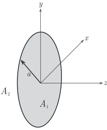
The general problem of the uniform-phase disk is defined as follows: the disk has a transmittance A1 and generates a phase shift ofβ to the portion of the plane wave

which passes through it, whereas the rest of the aperture plane has a transmittanceA2,

as shown in Fig. 3.1. A1 and A2 are, in general, complex arbitrary constants. Thus,

the aperture function U(r0) can be written as

U(r0) = (

A1exp(iβ), r0 ≤a

A2 , r0 > a

(3.1)

where a is the radius of the disk. Depending on the selected values of A1, A2, and

β, the aperture function in Eq. (3.1) can model different physical setups, such as a circular aperture (A1 = 1, β = 0) in a completely opaque plane A2 = 0, or an opaque

circular obstacle (A1 = 0, A2 = 1, β = 0), or a transparent plane A2 = 1 and a

transparent circular disk A1 = 1 with arbitrary phase shift β. Considering that the

aperture function U(r0) in Eq. (2.5) exhibits azimuthal symmetry, it is possible to

carry out the angular integral, which gives

Z 2π

0 dϕ0exp "

−ikr

z r0cos(ϕ0−ϕ)

#

= 2πJ0 −

kr z r0

!

. (3.2)

Substituting Eqs. (3.1) and (3.2) into Eq. (2.5), using the Bessel property

J0(−x) = J0(x), and removing the plane wave component yields

U(r;z) = ₋ik

z exp i k

2zr

2 ! (

A1exp(iβ) Z a

0 r0dr0exp i

k

2zr

2 0

!

J0

kr z r0

!

+A2 Z ∞

a r0dr0exp i

k

2zr

2 0

!

J0

kr z r0

!)

. (3.3)

The second integral in Eq. (3.3) can be completed so that it spans the complete radial coordinate, giving

U(r;z) = ₋ik

z exp i k

2zr

2 ! (

[A1exp(iβ)−A2] Z a

0 r0dr0exp i

k

2zr

2 0

!

J0

kr z r0

z y x a

A

A

Figure 3.1: Sketch of the uniform-phase disk aperture function.

+A2 Z ∞

0 r0dr0exp i

k

2zr

2 0

!

J0

kr z r0

!)

, (3.4)

where it is possible to identify the last integral as the 0th-order Hankel transform of the quadratic phase term,

Z ∞

0 r0dr0exp i

k

2zr

2 0

!

J0

kr z r0

!

= iz

k exp −i k

2zr

2 !

. (3.5)

After some simple algebraic manipulation, the diffraction pattern at some obser-vation point (r, z) is given by

U(r;z) =₋ika

2

z exp i k

2zr

2 !

[A1exp(iβ)−A2]I0(r, z) +A2, (3.6)

where

I0(r, z) = Z 1

0 ρ0dρ0exp i

ka2

2z ρ

2 0

!

J0

kar z ρ0

!

. (3.7)

2.5

0.5 1 1.5 2

z/L

4

0

U2

2.5

0.5 1 1.5 2

z/L

4

0

U2

(a)

(b)

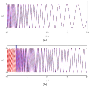
Figure 3.2: Axial intensity for a plane wave withλ = 632.8 nm diffracted by a circular aperture of radius (a)a = 500µm, and (b) a= 2500µm. The result from Eq. (3.6) is shown in blue, and the one from Eq. (3.8) is shown in red.

As a first validation of Eq. (3.6), the result from calculating the axial intensity of a unitary-amplitude plane wave with λ = 632.8 nm diffracted by a circular aperture, that is A1 = 1, A2 = 0, and β = 0, is compared with the exact solution published by

Dubra and Ferrari [18],

|U(0;z)_|2 = 1 + z

2

z2_+a2 −2

z

√

z2_+a2 cos  kz

 

s

1 + a

2

z2 −1   

, (3.8)

for two values of the aperture radiusa, and the results along the normalized longitudinal distance z/L are shown in Fig. 3.2. It can be seen from comparing Figs. 3.2(a) and 3.2(b) that the accuracy of equation Eq. (3.6) aroundz =L diminishes as the radius of the aperture increases. All the remaining diffraction patterns in this work were calculated using λ= 632.8 nm, unless otherwise specified.

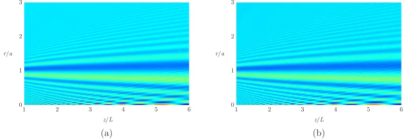
compared with the one calculated with Fourier propagation. In Fig. 3.3, a comparison in the axial intensity of the diffracted plane wave is shown. Furthermore, in Fig. 3.4 the intensity distributions for the propagation of the diffracted wave are shown for comparison. Finally, in Fig. 3.5, the phase distributions of the diffracted wave are shown for Eq. (3.6) in Fig. 3.5(a) and for Fourier propagation in Fig. 3.5(b). From Figs. 3.3 to 3.5, it is possible to observe that Eq. (3.6) exhibits good agreement with the results obtained with Fourier propagation for z/L _≥ 1, so numerically both methods can be considered equivalent in that range.

0

1 2 3 4 5 6

1 2 3

z/L

U2

Figure 3.3: Axial intensity for a circular π/5 phase mask of radiusa = 500µm.

1 2 3 4 5 6

z/L r/a

1 2 3

0

(a)

1 2 3 4 5 6

z/L r/a

1 2 3

0

(b)

Figure 3.4: (a) Intensity distribution of a plane wave diffracted by aπ/5 phase mask of radius a = 500 µm. (b) Intensity distribution of the same plane wave in (a) obtained by Fourier propagation.

1 2 3 4 5 6

z/L r/a

1 2 3

0

(a)

1 2 3 4 5 6

z/L r/a

1 2 3

0

(b)

Figure 3.5: (a) Phase distribution of a plane wave diffracted by a π/5 phase mask of radius a = 500µm. (b) Phase distribution of the same plane wave in (a) obtained by Fourier propagation.

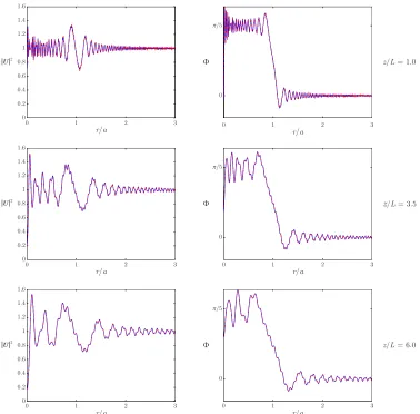
It can be seen from Fig. 3.6 that the results from expression Eq. (3.6) are in good agreement with those obtained from Fourier propagation up to a value of r/a. It is possible to see in Fig. 3.6 that as one moves further away from the aperture plane, that is as one increases z/L, the results from Eq. (3.6) remain accurate for larger values of

r/a, which is expected due to the nature of the Fresnel approximation. In other words, since for a given distance r from the propagation axis the subtended angle φ _≈ r/z

grows smaller as one moves further away alongz, it is also logical to assume that for a given subtended angleφthe maximum possible value ofr which lies within the Fresnel approximation increases as z does.

3.1

Non-unitary transmittances and Babinet’s

Prin-ciple

Fresnel diffraction of plane waves by circular apertures A1 = 1 and A2 = 0, and

circular obstacles A1 = 0 and A2 = 1 has been widely studied in the literature.

Fur-thermore, the case of a perfectly transparent disk with arbitrary phase shift β, that is A1 = A2 = 1 was analyzed in the previous section. Now, the more general case of

a uniform-phase disk with non-unitary transmittances, i.e. A1 6= 1 andA2 6= 1 with

arbitrary phase shift β, is considered.

Although the transmittances A1 and A2 are considered to be arbitrary

com-plex numbers, this research concentrates on real valued transmittances such that 0 _≤

A1, A2 ≤1, where a zero-valued transmittance indicates a completely opaque body, and

a unit-valued one represents a perfectly transparent body. In Fig. 3.7, the diffracted wave from a uniform-phase disk with A1 = 0.8, A2 = 0.4, and β = π/6 is shown for

0 1 2 3

r/a

0 1.6 1.4 1.2 1 0.8 0.6 0.4 0.2 U2

0 1 2 3

r/a

0 1 2 3

r/a

0 1.6 1.4 1.2 1 0.8 0.6 0.4 0.2 U2

0 1 2 3

r/a

0 1 2 3

r/a

0 1.6 1.4 1.2 1 0.8 0.6 0.4 0.2 U2

0 1 2 3

r/a

0 p/5 F 0 p/5 F 0 p/5

F z/L = 1.0

z/L = 3.5

z/L = 6.0

Figure 3.6: Intensity (left) and phase (right) of the diffracted wave atz =_{1.0,3.5,6.0_} for A1 = 1, A2 = 1 and β = π/5. Results from Eq. (3.6) are displayed in blue, and

Fourier propagation results in red.

the variations in the diffraction pattern due to propagation, the fact that the transmit-tances are different reflects itself in both the intensity _|U(r)_|2 and the phase Φ(r) of the diffracted wave, as a difference in the constant level of the pattern in the first case, and as a step-like structure located at the position of the amplitude discontinuity, that is at r/a= 1, in the latter one.

Now, the diffraction of plane waves by complementary aperture functions is studied as a way to numerically revise Babinet’s principle. According to Babinet’s principle, the sum of the complex amplitudes of waves diffracted by complementary screens equals the original wave without diffraction effects, which can be expressed as [2]

Uscreen+Ucomp= 1, (3.9)

func-3

0 1 2

r/a

0.8 0 U2 1 0.6 0.4 0.2 3

0 1 2

r/a

0

p/6

F

z/L = 1.0

z/L = 2.5

z/L = 4.0

Figure 3.7: Intensity (left) and phase (right) of the diffracted plane wave for A1 = 0.8,

A2 = 0.4, and β =π/6, observed at planes z/L={1.0,2.5,4.0}.

tion, and the plane wave component has been removed from both. Let UA1,A2 be

the diffracted pattern due to a plane wave passing through a uniform-phase disk with transmittances A1, A2, and phase shift β. In order to observe the result of Babinet’s

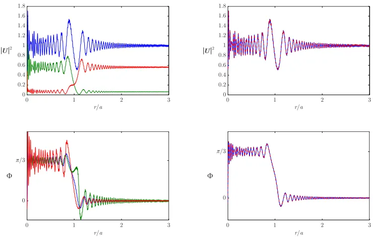
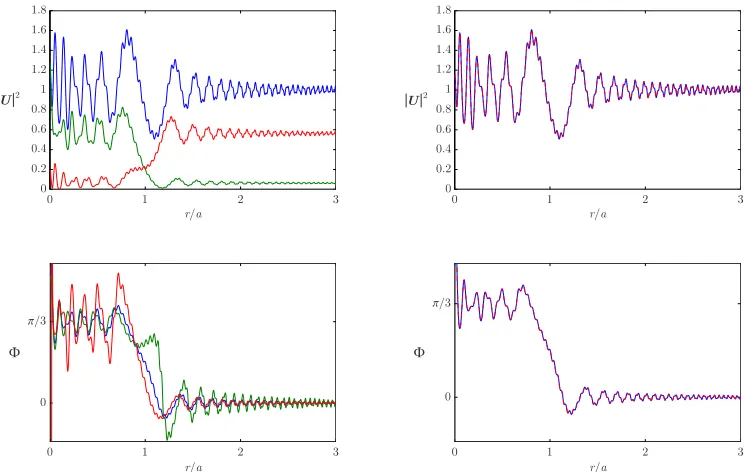
principle for a uniform-phase disk, the diffraction patterns were calculated for an aper-ture function with A1 = 3/4 and A2 = 1/4, and the complementary aperture function

withA1 = 1/4 andA2 = 3/4, both with a phase shiftβ=π/3. The diffraction patterns

of U3 4,

1 4, U

1 4,

3

4, and U1,1 are shown in Figs. 3.8 for z/L = 1.0, 3.9 for z/L = 3.0, and

3.10 for z/L= 5.0.

It can be seen from the right side of Figs. 3.8 to 3.10, that the sum of the complex amplitudes of the diffracted patterns caused by aperture functions with complementary values of their transmittances gives exactly the same result as a plane wave diffracted by an aperture function with unitary transmittances. Mathematically, this can be expressed in a simple equation,

UA1,A2 +U1−A1,1−A2 =U1,1. (3.10)

It is relatively easy to prove Eq. (3.10) parting from the diffraction integral in Eq. (3.3). As a simple abbreviation, let

I_ab =

Z b

a r0dr0exp i

k

2zr

2 0

!

J0

kr z r0

!

, (3.11)

so that the first and second radial integrals in Eq. (3.3) can be abbreviated as Ia

0 and

I∞

a respectively. Now, substituting the aforementioned notation into Eq. (3.3) gives

simplified expressions forUA1,A2 and U1−A1,1−A2,

UA1,A2 = − ik

z exp i k

2zr

2 !

[A1exp(iβ)I0a+A2I_a∞], (3.12)

U1−A1,1−A2 = − ik

z exp i k

2zr

2 !

3

0 1 2

r/a 0 U2 1.8 1.2 0.6 0.2 0.4 0.8 1 1.4 1.6 3

0 1 2

r/a 0 U2 1.8 1.2 0.6 0.2 0.4 0.8 1 1.4 1.6 0 p/3 F 3

0 1 2

r/a

0

p/3

F

3

0 1 2

r/a

Figure 3.8: (Left) Intensity and phase of the diffracted waves where U1,1 is shown in

blue, U1/4,3/4 in red, and U3/4,1/4 in green; (Right) Intensity and phase of the sum of

the complementary (blue) and A1 =A2 = 1 (red) cases at z/L= 1.0.

which are then substituted into the left member of Eq. (3.10) yielding

UA1,A2 +U1−A1,1−A2 = − ik

z exp i k

2zr

2 !

[A1+ (1−A1)] exp(iβ)I0a

+ [A2+ (1−A2)]I_a∞ )

= ₋ik

z exp i k

2zr

2 !

[exp(iβ)I0a+I

∞

a ]≡U1,1. (3.14)

On the other hand, if the values of the transmittances are exchanged in a second “complementary” aperture function, that is, for UA1,A2 and UA2,A1, the sum of the

diffraction patterns from both aperture functions gives the same pattern as a plane wave diffracted by an aperture function with unitary transmittances, except for a scale factor A1+A2,

UA1,A2 +UA2,A1 = (A1+A2)U1,1, (3.15)

and if A1+A2 = 1, then the result of Eq. (3.15) reduces to that of complementary

values of the transmittances in Eq. (3.10). Proof of Eq. (3.15) is obtained in a similar fashion to that of Eq. (3.10). Using the abbreviated notation introduced in Eq. (3.11), the new “complementary” complex amplitude can be expressed as

UA2,A1 =− ik

z exp i k

2zr

2 !

3

0 1 2

r/a 0

U2

1.8

1.2

0.6

0.2 0.4 0.8 1 1.4 1.6

3

0 1 2

r/a 0

U2

1.8

1.2

0.6

0.2 0.4 0.8 1 1.4 1.6

0

p/3

F

3

0 1 2

r/a

0

p/3

F

3

0 1 2

r/a

Figure 3.9: (Left) Intensity and phase of the diffracted waves where U1,1 is shown in

blue, U1/4,3/4 in red, and U3/4,1/4 in green; (Right) Intensity and phase of the sum of

the complementary (blue) and A1 =A2 = 1 (red) cases at z/L= 3.0.

and substituting Eqs. (3.12) and (3.16) into the left side of Eq. (3.15) gives

UA1,A2 +UA2,A1 = − ik

z exp i k

2zr

2 !

[(A1+A2) exp(iβ)I0a+ (A2+A1)I_a∞]

3

0 1 2

r/a 0

U2

1.8

1.2

0.6

0.2 0.4 0.8 1 1.4 1.6

3

0 1 2

r/a 0

U2

1.8

1.2

0.6

0.2 0.4 0.8 1 1.4 1.6

0

p/3

F

3

0 1 2

r/a

0

p/3

F

3

0 1 2

r/a

Figure 3.10: (Left) Intensity and phase of the diffracted waves where U1,1 is shown in

blue, U1/4,3/4 in red, and U3/4,1/4 in green; (Right) Intensity and phase of the sum of

Chapter 4

The finite-radius spiral phase plate

As mentioned previously in chapter 1, the Fresnel diffraction of several types of illumination through spiral phase plates has drawn much attention in the last few years. V. V. Kotlyar et al. recently focused on the diffraction of finite-radius plane waves through integer-step infinite spiral phase plates [10], whereas M. V. Berry studied the diffraction of ideal plane waves through integer- and fractional-step infinite spiral phase plates [9]. As an extension of the work of both V. V. Kotlyar and M. V. Berry, this chapter presents a detailed analysis of a finite-radius spiral phase plate (SPP) with ideal plane wave illumination, for an integer-sized step as a first stage, and for a fractional-sized step as the more general case.

4.1

Integer-step spiral phase plate

Following the definition from the previous chapter, the disk is replaced by a finite-radius spiral phase plate of integer-sized stepn, and arbitrary transmittance A1. The

rest of the aperture plane r > a presents a transmittance A2, as shown in Fig. 4.1.

Thus, the aperture function atz = 0 can be written as,

U(r0, ϕ0) = (

A1exp(inϕ0), r0 ≤a

A2 , r0 > a

(4.1)

where a is the radius of the spiral phase plate. Substituting Eq. (4.1) into Eq. (2.5), taking out the plane wave component, and separating the radial integral gives

U(r, ϕ;z) = ₋ ik

2πzexp i k

2zr

2 ! (

A1 Z a

0

r0dr0exp i

k

2zr

2 0

!

×

Z 2π

0 dϕ0exp "

−ikr

z r0cos(ϕ0−ϕ) +inϕ0

#

(4.2)

+A2 Z ∞

a r0dr0exp i

k

2zr

2 0

! Z 2π

0 dϕ0exp "

−ikr

z r0cos(ϕ0−ϕ)

#)

Chapter 4

The finite-radius spiral phase plate

As mentioned previously in chapter 1, the Fresnel diffraction of several types of illumination through spiral phase plates has drawn much attention in the last few years. V. V. Kotlyar et al. recently focused on the diffraction of finite-radius plane waves through integer-step infinite spiral phase plates [10], whereas M. V. Berry studied the diffraction of ideal plane waves through integer- and fractional-step infinite spiral phase plates [9]. As an extension of the work of both V. V. Kotlyar and M. V. Berry, this chapter presents a detailed analysis of a finite-radius spiral phase plate (SPP) with ideal plane wave illumination, for an integer-sized step as a first stage, and for a fractional-sized step as the more general case.

4.1

Integer-step spiral phase plate

Following the definition from the previous chapter, the disk is replaced by a finite-radius spiral phase plate of integer-sized stepn, and arbitrary transmittance A1. The

rest of the aperture plane r > a presents a transmittance A2, as shown in Fig. 4.1.

Thus, the aperture function atz = 0 can be written as,

U(r0, ϕ0) = (

A1exp(inϕ0), r0 ≤a

A2 , r0 > a

(4.1)

where a is the radius of the spiral phase plate. Substituting Eq. (4.1) into Eq. (2.5), taking out the plane wave component, and separating the radial integral gives

U(r, ϕ;z) = ₋ ik

2πzexp i k

2zr

2 ! (

A1 Z a

0

r0dr0exp i

k

2zr

2 0

!

×

Z 2π

0 dϕ0exp "

−ikr

z r0cos(ϕ0−ϕ) +inϕ0

#

(4.2)

+A2 Z ∞

a r0dr0exp i

k

2zr

2 0

! Z 2π

0 dϕ0exp "

−ikr

z r0cos(ϕ0−ϕ)

#)

y x z a

A

A

Figure 4.1: Sketch of the spiral phase plate aperture function.

The first angular integral in Eq. (4.2) is given by

Z 2π

0 dϕ0exp "

−ikr

z r0cos(ϕ0−ϕ) +inϕ0

#

=in2πexp(inϕ)Jn −

kr z r0

!

, (4.3)

and it is possible to identify the last angular integral in Eq. (4.2) as a special case of Eq. (4.3) forn= 0. Substituting Eq. (4.3) into Eq. (4.2), and using the Bessel identity

Jn(−x) = (−1)nJn(x) yields

U(r, ϕ;z) = ₋ik

z exp i k

2zr

2 ! (

A1exp(inϕ)(−i)n Z a

0

r0dr0exp i

k

2zr

2 0

!

Jn

kr z r0

!

+A2 Z ∞

a r0dr0exp i

k

2zr

2 0

!

J0

kr z r0

!)

. (4.4)

As in chapter 3, the last integral in Eq. (4.4) can be completed so that it spans the complete radial coordinate, yielding once again the 0-th order Hankel transform of the quadratic phase term, given in Eq. (3.5). After some simple algebraic manipulation, the diffraction pattern of a finite-radius spiral phase plate of integer stepn illuminated by an ideal plane wave is given by the simplified expression

U(r, ϕ;z) =₋ika

2

z exp i kr2

2z

!

[A1(−i)nexp (inϕ)In(r, z)−A2I0(r, z)] +A2, (4.5)

where

In(r, z) =

Z 1

0 exp i

ka2

2z ρ

2 0

!

Jn

kar z ρ0

!

and I0(r, z) is a special case of Eq. (4.6) for n = 0. Although there is no closed form

solution to Eq. (4.6), Kotlyar et al. published an analytical solution in terms of an infinite superposition of hypergeometric functions [10], given by

In(r, z) =

1

n!

ikar

2z

!n _∞ X

m=0

1

(2m+n+ 2)m!

ika2

2z

!m

× 1F2

 

2 + 2m+n

2 ,

4 + 2m+n

2 ,1 +n;−

kar

2z

!2

. (4.7)

Even though Eq. (4.7) is an analytical solution of Eq. (4.6), numerically it is not practical to use it for small distances, in the order of L, from the aperture plane due to the fact that the factor ka2_/2z

≫ 1. Thus, the partitioned Gaussian quadrature method remains to be more convenient to approximateIn(r, z) and I0(r, z).

n= 1 n= 2

z/L=1.0

z/L=2.5

z/L=4.0

U 2

F

F

Figure 4.2: Intensity and phase of the diffraction patterns at z/L= _{1.0,2.5,4.0_} for SPPs withn = 1 andn = 2.

n= 3 n= 4

z/L= 1.0

z/L= 2.5

z/L= 4.0

U 2

F

F

Figure 4.3: Intensity and phase of the diffraction patterns at z/L= _{1.0,2.5,4.0_} for SPPs withn = 3 andn = 4.

nm, and the transverse dimensions of the distributions are contained within square windows of width 3a, unless otherwise specified. As M. V. Berry showed in [9], the phase distribution of the diffracted waves hasnphase discontinuity lines symmetrically distributed with a separation of 2π/n, all of them presenting the ondulatory “decora-tion” mentioned by him. However, the main differences with Berry’s results are, first, that the phase discontinuity lines do not extend to r _{→ ∞}, but only up to r = a; second, that the topological charge, or total vortex strength, of the diffraction pattern is not concentrated in an-charge optical vortex at the origin, but in a variable number of charge _±1 optical vortices distributed around the origin, and third, that the total vortex strength of the pattern is alwaysSn= 0. These differences will be studied later

in more detail.

the effects on the topological characteristics are similar to those suffered by intensity. One of the more easily seen variations of the topological characteristics of the phase distribution is the reduction in the frequency of the ondulatory decoration along the phase discontinuity lines, which is obvious from Figs. 4.2 and 4.3.

4.1.1

Optical vortex distribution

One of the main concerns of this chapter is, besides the general intensity and phase distributions and their variations with changing order and propagation, is the vortex structure of the diffraction patterns generated by finite-radius spiral phase plates. In this section, the optical vortex distribution caused by spiral phase plates of integer-sized step n is studied, as well as the total topological charge of the diffracted wavefront.

In [10], Kotlyar et al. studied the spiral phase plate of integer-sized step n il-luminated by a finite-radius plane wave. The setup proposed by them is one of the cases which can be generated by adjusting the transmittances of the aperture plane, in this case, by setting A2 = 0. The intensity and phase distributions of the Fresnel

diffraction pattern generated by this setup for n = 3 , namely A1 = 1, A2 = 0, and

n = 3, can be seen in the first column of Fig. 4.4. However, since the intention of this research is to study a more general situation, it is shown in the rest of Fig. 4.4 how the Fresnel diffraction pattern gradually loses its azimuthal symmetry and gains a spiral-like structure as the outer transmittance A2 is varied from 0 to 1.

A

= 0

U

A

= 0.25

A

= 0.5

A

= 0.75

A

= 1

F

Figure 4.4: Intensity and phase of the diffraction pattern at z/L= 1.0 for a SPP with

n= 3 as A2 varies from 0 to 1.

that was previously contained only within the phase of the diffracted wavefront. How-ever, the consequence of having light without a phase shift interfering with light having a spiral phase structure is not only a deformation in the intensity of the diffracted pattern, but also the fact that the phase discontinuity lines lose their spiral behavior forr > a, as it can be seen from the lower row of Fig. 4.4. Due to this interference, the phase discontinuity lines which were supposed to extend to r_{→ ∞} now only reach up to r = a, as mentioned at the end of the previous section. This causes the birth of n

new optical vortices that did not exist before, which in turn modifies the total vortex strength of the wavefront.

The total vortex strength of a light distribution is the signed sum of all the vortices threading a large loop including thez axis, namely

Sn = lim r→∞

Z 2π 0 dϕ

∂

∂ϕΦ(r), (4.8)

where as previously stated, Φ(r) is the phase distribution of the diffracted wavefront. The number of vortices contained in the phase distribution of a plane wave diffracted by a SPP changes as the outer transmittance is varied from 0 to 1. It is possible to see in the first row of Fig. 4.5, that for z/L= 1.0 when a n = 1 spiral phase plate is illuminated by a finite-radius plane wave, i.e. A2 = 0, the total vortex strength S1 = 1

is concentrated in a central vortex on thez axis. As more light is allowed to interfere, that is as A2 varies from 0 to 1, two things happen: first, a new vortex is born at the

border of the SPP due to the finite length of the phase singularity line, and second, the central vortex splits up into a variable number of_±1 vortices which remain close to the propagation axis as shown in the second and third rows of Fig. 4.5. Because the newly born negative outer vortex cancels out the one positive inner vortex which survives opposite-sign cancelation near the axis, the total vortex strength S1 is nullified, thus

S1 = 0 for any value ofA2 >0.

This behavior is not limited to the n = 1 SPP, as it takes place in a very similar fashion for SPPs withn >1, with two important differences, the first one being that the number and distribution of the strength _±1 vortices into which the strength n central vortex for A2 = 0 splits up become larger and much more complicated respectively as

the topological charge n of the SPP increases, and the second one being that instead of one negative outer vortex, there are n outer unit strength negative vortices which cancel out with n surviving inner unit strength positive vortices, causing Sn = 0 for

any value of the SPP topological charge n. Since the topological charge of the spiral phase plate can be either a positive or negative integer, when n < 0 the signs of all the vortices mentioned previously are switched. In other words, the surviving inner vortices are negative and their signed sum equals _{− |}n_|, and in consequence, the _|n_|

p -p

A = 02

A = 0.52

3a a/5

A = 12

Figure 4.5: Location and sign of optical vortices present in the phase distribution of a plane wave diffracted by a SPP withn = 1 forA2 ={0,0.5,1}, observed atz/L= 1.0.

In the right column, the nodal lines Re_{U_} = 0 and Im_{U_} = 0 are displayed in red and blue respectively, to make the position of the vortices easier to determine.

Besides changes in the outer transmittance A2 and the magnitude of the SPP

topological chargen, spatial propagation is the other factor which influences the number and distribution of unit strength vortices within the transverse phase distribution of the diffracted wavefront. As the diffracted wave propagates along the z axis, the number of unit strength vortices varies non-uniformly, that is, pairs of _±1 vortices are created and annihilated constantly as the profile travels farther away from the aperture plane. Although there is no uniform behavior, there exist a general tendency regarding the creation-annihilation process of the optical vortices observed in the phase distribution. Since the total vortex strength of the diffracted wavefront is Sn = 0 for any value

3a z/L=1.0

z/L= 15

z/L= 25

U2 F

z/L=110

3a

3a

5a

Figure 4.6: Location and sign of optical vortices present in the phase distribution of a plane wave diffracted by a SPP with n = 1 for A2 = 1, observed at z/L =

{1.0,15,25,110_}. In the right column, the nodal lines Re_{U_}= 0 and Im_{U_} = 0 are displayed in red and blue respectively, to make the position of the vortices easier to determine.

their corresponding phase discontinuity line. Furthermore, as wavefront moves along the z axis, the n inner optical vortices gradually move away from the propagation axis toward their corresponding outer vortices, shortening the phase discontinuity lines until the vortices reach each other and cancel out when the pattern approaches the far-field regime, resulting in a diffraction pattern which contains no optical vortices, in agreement with the value of its total vortex strength Sn = 0. This behavior of the

optical vortex distribution under propagation can be observed in Fig. 4.6, where the first row shows the intensity and phase of the diffraction pattern at z/L = 1.0 for

A2 = 1, and the detailed vortex distribution for that value of the propagation distance

the aperture plane, the distribution of the optical vortices can be appreciated without any close-up, as visible in the right columns of the last three rows of Fig. 4.6, where the location and sign of the vortices is indicated.

a

/4

I

II III IV

V

Figure 4.7: Trayectory of the inner vortices during propagation from z/L= 5.0 up to

z/L= 50.0 for a plane wave diffracted by a 500 µm SPP with n = 1. The red circles mark a pair-annihilation event, whereas the blue circles indicate a pair-creation.

Finally, in Fig. 4.7 it is possible to see the trayectory of the inner vortices upon propagation in the range 5.0_≤z/L_≤50.0 for a 500µm spiral phase plate withn = 1. Although lines closer to the origin do not necessarily mean that the motion happened earlier in the propagation process, in general it can be observed that as the observa-tion plane moves away from the aperture plane, that is as the normalized distancez/L

4.2

Fractional-step spiral phase plate

The general case of a spiral phase plate with fractional-sized step α can be ex-pressed in a very similar manner to that of the integer-sized step analyzed in the previous section. The spiral phase plate has an arbitrary transmittance A1, and

in-duces a phase shift exp(iαϕ0) on the light which passes through it. The rest of the

aperture plane presents a constant transmittance A2. This can be summarized in a

simple mathematical expression given by,

U(r0, ϕ0) = (

A1exp(iαϕ0), r0 ≤a

A2 , r0 > a

(4.9)

where as before, a is the radius of the spiral phase plate. Substituting Eq. (4.9) into Eq. (2.5), taking out the plane wave component, and separating the radial integral yields

U(r, ϕ;z) = ₋ ik

2πzexp i k

2zr

2 ! (

A1 Z a

0 r0dr0exp i

k

2zr

2 0

!

×

Z 2π 0

dϕ0exp "

−ikr

z r0cos(ϕ0−ϕ) +iαϕ0

#

(4.10)

+A2 Z ∞

a r0dr0exp i

k

2zr

2 0

! Z 2π

0

dϕ0exp "

−ikr

z r0cos(ϕ0−ϕ)

#)

,

which is very similar to Eq. (4.2), except for the fact that α now plays the role of n. However, as trivial as this change may seem, becauseαis an arbitrary real number, the first angular integral in Eq. (4.10) has no closed form solution for arbitrary values ofϕ0.

However, it is possible to obtain a complex Fourier series expansion of the exp(iαϕ0)

term, which is given by [9]

exp(iαϕ0) =

exp(iαπ) sin(απ)

π

∞

X

m=−∞

exp(inϕ0)

α₋m . (4.11)

Substituting the Fourier series expansion Eq. (4.11) into Eq. (4.10), removing the plane wave component, using the integral definition of the n-th order Bessel function given in Eq. (4.3) and the identities Jn(−x) = (−1)nJn(x) and i−nJ−n(x) = inJn(x),

yields

U(r, ϕ;z) = ₋ik

z exp i k

2zr

2 ! (

A1

exp(iαπ) sin(απ)

π

×

∞

X

m=−∞

(₋i)|m|

α₋m exp(imϕ)

Z a

0 r0dr0exp i

k

2zr

2 0

!

J|m|

kr z r0

!

(4.12)

+A2 Z ∞

a r0dr0exp i

k

2zr

2 0

!

J0

kr z r0

!)

As it has been done previously, the last integral in Eq. (4.12) is completed to span the complete radial coordinate, so that it becomes the 0-th order Hankel transform given in Eq. (3.5). After doing some simple algebra, the Fresnel diffraction pattern caused by a finite-radius spiral phase plate with fractional-sized stepαwhen illuminated by an ideal plane wave is given by the simplified expression

U(r, ϕ;z) =₋ika

2

z exp i k

2zr

2 ! _∞

X

m=−∞

Cmexp(imϕ)I|m|(r, z) +A2, (4.13)

where

Cm =A1

(₋1)α_sin(απ)

π

(₋i)|m|

α₋m −A2δm,0, (4.14)

and I|m|(r, z) is given by an expression similar to Eq. (4.6), save for a simple variable

substitution n_{→ |}m_|,

I|m|(r, z) =

Z 1

0 exp i

ka2

2z ρ

2 0

!

J|m|

kar z ρ0

!

ρ0dρ0. (4.15)

It is possible to see that Eq. (4.13) is in fact a general expression for the Fresnel diffraction pattern of a finite-radius spiral phase plate of arbitrary real topological chargeα, since the case of integer topological charge nis also covered by it. In order to show that, the limit of theα-dependent term of expansion coefficientsCm whenα →n

is observed,

lim

α→n

"

(₋1)α_sin(απ)

π(α₋m)

#

=

(

1, for m=n

0, for m₆=n (4.16)

so it is possible to expressCm as

Cm|α=n =A1(−1)|m|δm,n−A2δm,0, (4.17)

where δm,n is the Kronecker delta. It can be easily seen that substituting Eq. (4.17)

into Eq. (4.13) yields the same expression as Eq. (4.5) for n _≥0. For n <0 it is just a matter of invoking the Bessel identity under sign change in the order to obtain the same result.

a =

 1

a =

 1.25

a =

 1.5

a =

 1.75

a =

 2

Figure 4.8: Intensity and phase of the diffraction pattern at z/L = 1.0 for α =

{1,1.25,1.5,1.75,2}.

the diffraction waves caused by the border of the spiral phase plate. As the topological

charge α increases from n to n + 1, a new dark lobe originates from the dark stripe

along the positive x axis and begins to extend into the corresponding spiral orientation.

In Fig. 4.8 it is possible to see how the dark stripe forms as soon as α becomes larger

than n = 1, and as the topological charge increases the second spiral lobe gradually

grows out from the end of the dark stripe at x = a. This process continues until α

approaches n = 2, and the dark stripe diminishes its size as the second spiral lobe is

fully formed. In a similar fashion, the phase distribution of the diffraction pattern gains

a new "helix" when α increases from 1 to 2. In the lower row of Fig. 4.8 it is easy to see

how the second phase helix begins to form as α increases, and when α = 1.5, the phase

discontinuity line begins to emerge at the positive x axis, generating several vortices

along it, and the helix continues to grow until it reaches its complete form when α = 2.

Just as it happens when α is an integer, the intensity and phase distributions

of the Fresnel diffraction pattern change both in size and shape through propagation. Figures 4.9 and 4.10 show the intensity and phase of the Fresnel diffraction pattern at

three different values of z/L for SPPs with α = {1.5, 2.25} and α

axis. The phase of the diffracted wavefront behaves similarly, as the oscillatory dec-z/L = 1.0

z/L = 2.5

z/L

 = 4.0

Figure 4.9: Intensity and phase of the diffraction patterns at z/L = {1.0,2.5,4.0} for

SPPs with α = 1.5 and α = 2.25 fractional-sized steps.

orations become more defined and reduce their frequency. Furthermore, the vortical

structure near the z axis becomes larger and easier to observe as the observation plane

moves away from the aperture one.

4.2.1 Optical vortex distribution for

α n

 + 1/2

The optical vortex distribution is quite different when α is an arbitrary fractional

number than when α is a half-integer. First, the situation when  α = 6 n + 1/2 is studied

in detail, including the differences between the cases when n < α < n + 1/2 and

n + 1/2 < α < n + 1.

In Fig. 4.11, the variations in the intensity and phase of the Fresnel diffraction

pattern for α = 3.3 are shown for different values of A₂ such that 0 < A₂ < 1. It is

possible to see a similar behavior to that observed in Fig. 4.4: the intensity profile of the diffracted wavefront gradually loses the azimuthal pseudo-symmetry and gains a

spiral-like structure, save for the dark stripe along the positive x axis which remains

almost unchanged. The phase distribution is also modified since the phase discontinuity lines, which had a spiral behavior up to r outside the spiral phase plate, now have

a finite extent reaching up to r = a as in the integer-step case. Thus, as previously,

n = 3 new vortices are born at the border of the SPP. Once again, this behavior applies

to any value of α < n + 1/2.

z/L = 1.0

z/L = 2.5

z/L = 4.0

α = 2.85 α = 3.5

Figure 4.10: Intensity and phase of the diffraction patterns at z/L = {1.0, 2.5,4.0} for

SPPs with α = 2.85 and α = 3.5 fractional-sized steps.

On the other hand, in Fig. 4.12 the variations in the intensity and phase of the

Fresnel diffraction pattern for α = 3.6 are shown for different values of A₂. It is easy to

see that the behavior of the intensity variations is the same as the previous example: a deformation of the intensity distribution into a spiral-like structure with the dark

horizontal stripe remaining unmodified. The only difference between the α < n + 1/2

and the α > n + 1/2 cases is the length of the dark spiral lobe extending from the

end of the dark stripe, since for α < n + 1/2 it subtends an angle less than π/n and

for α > n + 1/2 it does so for more than π/n. The difference between both ranges becomes more evident in the phase distribution of the diffraction pattern, since for α < n + 1/2 there are only n visible phase discontinuity lines and the (n + 1)-th helix

is just beginning to form, whereas for α > n + 1/2 there are n + 1 phase discontinuity

lines and the (n + 1)-th helix is more than halfway completed.

Just as with the spiral phase plates of integer topological charge, propagation is an important factor which greatly alters the location and number of optical vortices contained in the phase of the diffracted wavefront. Figures 4.15 and 4.16 show the effect of propagation on the distribution of the optical vortices for plane waves diffracted by

spiral phase plates of α = 1.4 and α = 1.8 respectively. For z/L = 1.0 it is not possible

to appreciate the optical vortices near the z axis in the first row of the aforementioned

Figure 4.11: Intensity and phase of the diffraction pattern at z/L  = 1 . 0 for a SPP with

α = 3.3 when A2 varies from 0 to 1.

near the propagation axis, where it is possible to observe the location and sign of the optical vortices. It is possible to see in Figs. 4.13 and 4.14 that the fractional phase discontinuity in the origin of the aperture plane splits up into several unit-strength

vortices near the z axis, for both A₂ = 0 and A₂ = 1. Once again from Figs. 4.15 and

4.16, it can be seen that there is always an even number of vortices during propagation,

which immediately implies that the total vortex strength of the diffracted wave is Sα = 0

for any value of α. As with the integer-step spiral phase plates, the reason for the null topological charge of the optical wavefront is the presence of the outer vortices caused by interference of the portion of the plane wave which suffered no phase shift. The fact that the total vortex strength remains to be zero during propagation allows to assume that regardless of the number of optical vortices near the aperture plane, the general tendency is for them to gradually cancel out in pairs through propagation, so that the diffraction pattern on the far-field regime will present no optical vortices at all, as can be observed in the last row of Figs. 4.15 and 4.16.

4.2.2 Optical vortex distribution for

α = n

 + 1/2

According to Berry, the passing of α through a half-integer is the mechanism

through which a new vortex is born, and in turn through which the total vortex strength

increases an integer so that Sα is the integer nearest to α. In this work, the passing

of α through a half-integer does not increase the value of the topological charge of

the wavefront since it marks the birth of a pair of opposite-sign vortices, one near the

propagation axis with the same sign as α, and one at the border of the SPP with

the opposite sign. In [9], Berry predicted that there would be an infinite number of

A

=

0

Figure 4.12: Intensity and phase of the diffraction pattern at z/L  = 1 . 0 for a SPP with

a = 3.6 when A₂ varies from 0 to 1.

cancelation process of these vortices would leave one additional vortex when α > n+1/2.

The main difference between Berry's argument and this research is the fact that the

number of vortices along positive x axis is not infinite due to the finite radius of the

spiral phase plate. Thus, the cancelation process of those newly born vortices leaves

not one, but two additional vortices of opposite sign so that the topological charge S_α

remains constant and equal to zero. In other words, when α approaches n + 1/2 from

below, the chain of vortices starts to appear until the maximum number of vortices is

reached when α = n + 1/2. Then, as α begins to increase, the chain of vortices begins

to cancel itself, but in a different manner as it appeared, so that the two new vortices survive the annihilation process.

Furthermore, the optical vortices along the positive x

 axis also suffer the annihi-lation tendency caused by spacial propagation. In the first two rows of Fig. 4.17, it is

possible to see in the close-up that as the observation plane moves from z/L = 1.0 to

z/L = 5.0, the number of optical vortices along positive x axis diminishes dramatically,

even more so than the ones located near the propagation axis. Following the same line of thought used in the analysis of the behavior of optical vortices through propagation, it is easy to see from the last two rows in Fig. 4.17 that as the diffracted wavefront moves farther away from the aperture plane and closer to the far-field regime, its phase singularities suffer the annihilation process previously observed and analyzed in the Fresnel diffraction patterns generated by finite-radius integer-step spiral phase plates. Once again, all the optical vortices must disappear as the observation plane moves into

the far-field region because the total vortex strength S_α = 0 must remain constant, and

A2= 0

A2=1

Figure 4.13: Location and sign of optical vortices in the diffraction pattern at z/L = 1.0

for a SPP with α = 1.4 and A₂ = {0,1}. In the right column the nodal lines Re{U} = 0

and Im{U} = 0 are displayed in red and blue, respectively.

A2= 0

A2=1

Figure 4.14: Location and sign of optical vortices in the diffraction pattern at z/L = 1.0

for a SPP with α = 1.8 and A₂ = {0,1}. In the right column the nodal lines Re{U} = 0

Figure 4.15: Intensity and phase of the diffraction pattern at z/L = {1.0,15, 25,110}

for a SPP with α = 1.4 and A₂ = 1. In the right column the nodal lines Re{U} = 0

Figure 4.16: Intensity and phase of the diffraction pattern at z/L = {1.0,15, 25,110}

for a SPP with α = 1.8 and A₂ = 1. In the right column the nodal lines Re{U} = 0

Figure 4.17: Intensity and phase distributions of the diffracted wave caused by a SPP

Chapter 5

Conclusions

The main purpose of this work was to study the problem of Fresnel diffraction of ideal plane waves by circular phase objects of finite radius. First, the finite-radius uniform-phase disk was analyzed as a first stage, and an expression for the diffraction pattern in terms of a radial integral was found. One of the main results obtained through the analysis of the uniform-phase disk was a new alternative formulation of Babinet’s principle, so that the diffraction patterns of screens with complementary val-ues of their transmittances can be obtained from one of the knowledge of the pattern corresponding to one of the screens and of the pattern generated by a unitary transmit-tance screen. The main difference between this alternative formulation and the classic formulation found in most textbooks is the fact that the sum of the complex amplitudes of the patterns corresponding to complementary screens gives the diffraction pattern for unitary transmittances, instead of the already known result of the sum being equal to the original plane wave illumination. However, the purpose of studying the uniform-phase disk was mainly to validate the numerical techniques which were to be applied to the more complex problem of the spiral phase plate. According to the results shown in chapter 3, the partitioned Gaussian quadrature used to calculate the Fresnel diffraction patterns gave results which can be considered to be numerically equivalent to Fourier propagation for the whole range of validity of the Fresnel approximation, as long as the radius of the phase object is not too large. The results were shown to be in excellent accordance with the ones given by Fourier propagation for disk radii of several hundreds of micrometers, so for the rest of the document a standard radius of a = 500 µm was chosen to ease the comparison of the results obtained.