Dollar strength, peso vulnerability to sudden stops: a perfect foresight model of Argentina's convertibility

Universidad Nacional de La Plata

Novenas Jornadas de Economía

Monetaria e Internacional

La Plata, 6 y 7 de mayo de 2004

Dollar Strength, Peso Vulnerability to Sudden Stops: A Perfect

Foresight Model of Argentina's Convertibility

Dollar strength, Peso vulnerability to Sudden Stops

A perfect foresight model of Argentina’s Convertibility

1

Guillermo J. Escudé

Central Bank of Argentina

March, 2004

_________________________________________________________________________

1

Research Department, Central Bank of Argentina. The views contained in this paper are solely the author’s and are not meant to reflect those of the authorities of the Central Bank of Argentina. Research assistance by Juan Martín Sotes Paladino is gratefully

Dollar strength, Peso vulnerability to Sudden Stops: a perfect foresight model

of Argentina’s Convertibility

Guillermo Escudé

This paper presents a model designed to study the dynamic response of the economy under a fixed peg to the dollar to an international (and exogenous) real appreciation of the dollar, when there is wage and price stickiness, perfect capital mobility subject to sudden stops, and predominantly dollar denominated foreign debts with predominantly non-dollar trade. Assuming perfect foresight, we take the simple case in which the world is composed of the U.S.A., Europe, and Argentina and while all foreign debts are dollar denominated, all foreign trade is done with Europe. Hence, an important parameter in the model is the exogenous euro/dollar real exchange rate. PPP prevails in the export sector and there is monopolistically competitive price setting in the domestic sector and monopolistically competitive wage setting by households. Both are subject to adjustment cost functions that generate stickiness and domestic price and wage gaps, which result in ‘Phillips curve’ equations for domestic prices and wages, respectively. Money demand is generated by a transactions technology. The first order conditions for firms and households under symmetric monopolistic competition equilibriums and the budget constraints result in a four dimensional dynamical system in the multilateral real exchange rate (MRER), the real wage, the rate of domestic price inflation and the rate of wage inflation. This system has a saddle-path stable equilibrium which is dependent on the marginal utility of wealth. Under the assumption that the economy is what is called a Domestically Biased Economy in Production relative to Consumption (DBE), it is seen that strong dollar shocks, which require an inter-temporally smoothened fall in consumption (and hence an increase in the marginal utility of wealth), have perverse impact effects. The peso appreciates in real terms and the real wage increases. These effects generate foreign indebtedness and increased vulnerability to (exogenous and unexpected) sudden stops. The DBE assumption essentially entails that real depreciations require reductions in the real wage to preserve (long run) labor market equilibrium. A story is developed to explain the main features of the functioning and ultimate collapse of Convertibility in Argentina, by assuming a strong dollar shock which is believed to be temporary and has the effect of generating

unemployment, recession and debt accumulation. But before the new steady state is reached it is revealed that the shock is permanent, which triggers a sudden stop, a default, a

devaluation, a debt restructuring, fiscal reform, and the return to capital market access. A more flexible exchange regime could avoid the debt accumulation that triggers the sudden stop, as well as the long period of unemployment, recession, and deflation.

Key words: multilateral real exchange rate, fixed exchange regime, strong dollar shock, sudden stops

JEL: F41, F31, E52, E32

1

Dollar strength, Peso vulnerability to Sudden Stops: a perfect foresight model

of Argentina’s Convertibilit y

Guillermo Escudé

January, 2004

“Non ridere, non lugere, neque detestari, sed intelligere”. Spinoza

I. Introduction

Argentina’s experience with Convertibility, a very hard peg to the U.S. dollar, ended in catastrophe after very significant shocks that were not adequately addressed through credible policy changes. In the initial phase of the monetary/exchange regime, disinflation was achieved quickly (after two bouts of hyperinflation) with no output cost. Quite the contrary, high rates of output growth were quickly achieved, giving the regime an aura of success that made it exceedingly popular both domestically and abroad. The initial phase ended with the Tequila crisis, a pure contagion effect that triggered a run on the currency and the banking system, putting the regime’s resilience to test. After a three quarter recession, the economy was growing briskly again, and this increased the domestic

consensus on the merits of the regime. However, during its second phase, the Convertibility regime had to face a much more severe test through a series of shocks that eventually led to the regime’s collapse. The most significant of these shocks were 1) the dollar appreciation after mid-1995, which had an especially dramatic impact when Argentina’s main trade partner, Brazil, devalued in January 1999, but when looked at with historical perspective was just a blip in a period of real appreciation of the peso (Figure A5), 2) the reduction in the availability of external funds for emerging market economies since 1996, and especially after the Russian crisis in August 1998, which increased yield spreads over U.S. Treasury bonds of emerging sovereign bonds (Figure A22), and 3) the fall in the price of agricultural commodities subsequent to the Asian crisis in 1997 which generated a significant

1

Research Department, Central Bank of Argentina. The views contained in this paper are solely the author’s and are not meant to reflect those of the authorities of the Central Bank of Argentina. Research assistance by Juan Sotes Paladino is gratefully acknowledged.

2

deterioration in Argentina’s terms of trade. This shock, however, was much less persistent than the other two.

After three and a half years of recession, there was a sudden stop in the roll-over of public debt amortizations and a massive run on the banking system and the currency.

Convertibility of deposits to cash was suspended, causing furious street demonstrations that ultimately led to the resignation of the President (the Vice-President had resigned 6 months earlier), the declaration of default on the government debt, a devaluation, and the

administrative conversion (to pesos) of the currency denomination of dollar bank loans and deposits. Unemployment, which had been steadily increasing since the early 90s, reached a peak of 21.5%. This figure, however, does not completely reflect the magnitude of the social tragedy. When converted to reflect the hourly underemployment of those employed, the unemployment rate reaches more than 30% (Figure A3). Real manufacturing wages, which had been relatively constant during the 90s, fell dramatically after the devaluation (Figure A4). Most of the growth experienced during the initial phase of the regime was subsequently undone through the protracted recession that began in the second half of 1998. Much has been said trying to determine the principal culprits of the crisis. Many have emphasized the role of fiscal policies (Mussa (2002)). It is certainly true that some fiscal looseness (including court decisions on past claims on the government) as well as the up-front costs of the 1994 pension reform and the effects of the long recession on tax

collection increased the public debt from 29% of GDP in 1993 to 51% in 2001, and that this increased the vulnerability of the economy to the external shocks that it was facing. But there is increasing consensus on the importance of the monetary/exchange rate regime in explaining the run up to the crisis through the severe handicap it generated as to the possibility of correcting for the gradual but steady loss of competitiveness.

influences on the appreciation of the peso.3 The dynamics of the former has been studied, for example, by Calvo and Végh (1992). But the consequences of strong dollar shocks on competitiveness under inflation inertia and dollar pegs is seldom even mentioned even though it is very relevant empirically.

This paper presents a model designed to study the dynamics of a fixed exchange (or fixed crawling peg) regime under wage and price stickiness and to address some of the principal characteristics of an economy such as Argentina’s: a small open economy that faces

parametric prices in trade and is highly dependent on external finance; an economy which was financially highly dollarized but where the origin and destiny of its trade is highly diversified; an economy which, after a decade of high inflation in the 80s, by means of an exchange rate anchor returned to a more normal situation of “sticky” nominal wages and prices. To streamline the asymmetry between the diversification of trade partners (and currencies) and the financial dollarization, we take the extreme case in which the world is composed of the U.S.A., Europe, and Argentina, and while all of Argentina’s foreign debts are dollar denominated, all its trade is done with Europe.4 Hence, an important parameter in the model is the exogenous euro/dollar bilateral real exchange rate, ρ, which can

empirically be measured by the Fed’s Real Broad Dollar Index. The latter typically presents long phases of appreciation and depreciation (Figure A1). Hence, when the strong dollar phase begins it is probable that the appreciation will get gradually more pronounced and that this will persist during a number of years. Producers in a country that peg their currency to the dollar hence find it increasingly difficult to compete domestically with imported goods or in foreign markets unless their increase in productivity is sufficiently fast to compensate for the real appreciation (or trade policy is specially geared to

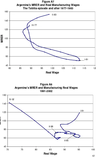
compensate for this). The importance of the parameter ρ (“dollar strength”) is highlighted by the Argentine experience during the last two periods in which it pegged to the dollar: the “tablita” experience of 1979-81 and the extended Convertibility experience in 1991-2001 (Figure A5). In both episodes, international dollar appreciations combined with a domestic

3

As Figures A5 and A7 show, the “tablita” experience of the late 70s, in which there was a crawling peg to the dollar, took place in the midst of an important strong dollar shock. Although the episode was shorter, the real appreciation was even bigger than under Convertibility and the experience also ended with a triple crisis (as well as the Malvinas/Falklands war and the concomitant demise of the military regime).

predetermined exchange rate regime that pegged the peso to the dollar, as well as with a process of financial liberalization, ended in an abrupt triple crisis (debt, currency and banking).

This paper shows that for a country with asymmetry in the currency denomination of its financial vis a vis trade transactions, the exogenous bilateral real exchange rate between its partners (ρ) is one of the fundamental determinants of the multilateral real exchange rate (MRER). In the application to Argentina, permanent dollar appreciations have the effect of requiring a more depreciated peso, in real terms, in the long run. But a hard peg to the dollar obstructs a timely adjustment of the MRER in the required direction if there are sticky prices and wages, as is typically the case. Even worse, in economies where labor market clearing gives an inverse relation between the MRER and the real wage (economies labeled Domestically Biased in Production relative to Consumption –DBEs- in this paper) the impact effects of permanent real dollar appreciations are perverse, in the sense that they go in the wrong direction: while they appreciate the peso in real terms and increase the real wage, the opposite occurs with the steady state values of these variables.

We call DBEs those economies in which a real currency depreciation requires a lower real wage to clear the labor market because the resulting shift of labor from the domestic to the export sector is smaller than the shift of consumption from imports to domestic goods. Hence, in such economies a real depreciation of the currency, given the real wage, reduces total labor demand, requiring a reduction in the real wage to attain labor market

equilibrium. We prove that in such economies an increase in the marginal utility of wealth, which is a direct consequence of the inter-temporal adjustment of households to a strong dollar shock, has the unequivocal effect of increasing the steady state value of the MRER and reducing the steady state value of the real wage, i.e. the opposite to the impact effects of the strong dollar shock. Hence, even if the strong dollar shock is temporary, due to its negative wealth effect it has perverse long run effects on the MRER and the real wage. It is assumed that PPP prevails for producers in the export sector and that there is price setting in the domestic sector based on monopolistic competition. There is also

make domestic sector firms and households adjust prices and wages gradually towards their desired long run levels. These long run levels are those that prevail in the benchmark economy of fully flexible prices and wages (cfr. Woodford (2003)). The corresponding dynamical equations can be interpreted as Phillips curves, for domestic prices and wages, respectively. This results in a four dimensional dynamical system which has a saddle-path stable equilibrium. The eigen-values are necessarily all different, but they may be real or complex. The system is graphed in two dimensions using the dominant eigen-vector method used by Calvo (1987).

With this scaffolding, a story is developed in order to explain the main features of the evolution and ultimate collapse of Convertibility in Argentina, within the limitations imposed by a perfect foresight model. We assume there is a first shock which is

unanimously considered to be temporary: an appreciation of the dollar vis a vis the euro. This has the effect of generating unemployment and recession and putting the economy on a path that slowly leads to the new steady state and during which capital markets are used to finance the transition. However, before this (long) process is over there is a new shock, which is the revelation that the dollar appreciation is more persistent than was expected. To simplify, we assume that it is revealed that the shock is permanent. This triggers a sudden stop in finance, since all debts are assumed to be of instant maturity and investors are not willing to finance the much bigger shock without forcing a substantial change in domestic policies. This change comes about through a default, a haircut on foreign debts, the

government assumption of certain inter-private debts, a devaluation, and fiscal reform. This disruption, however, has the consequence of making international capital markets again accessible to the domestic economy.

The model implies that it is far better to devalue right after the initial shock, avoiding the long period of unemployment and recession financed with foreign debt. With such a timely policy change that avoids increased indebtedness, the second shock might fail to trigger a sudden stop, if what triggers the sudden stop is a threshold foreign debt level that is only known to foreign investors (or not even known to any one of them individually). Given the credibility problems with soft pegs, the model also has the implication that a fixed

such a regime is inferior to more flexible exchange regimes where changes in the nominal exchange rate compensate for much of the wage and price stickiness. Indeed, if the “hard fix corner” is optimal for any economy (cfr. Fischer (2001) and Edwards (2000)), it is certainly sub-optimal for DBEs that have a marked asymmetry in the currency

denominations of financial and trade transactions, as the Argentine experience painfully illustrates.

II. The model

II.1. The recessionary and debt generating consequences of dollar appreciations in a nutshell

Households and the government are assumed to consume imported and domestic goods (i.e. goods that are produced domestically and only consumed domestically). Hence, it is convenient to define the (consumption) multilateral real exchange rate (MRER) as the relative price between Argentine imports (M) and Argentine domestic goods (N). To simplify, it is assumed that all trade is done with Europe (which stands for all trade partners other than the U.S.A.). Hence, the MRER is reduced to Argentina’s bil ateral real exchange rate with Europe:

(1) e ≡ PM/PN≡ (E/ρ)PM*/PN = E/(ρPN). ( PM*= 1 )

where E is Argentina’s nominal exchange rate (pesos per dollar), ρ is Europe’s nominal exchange rate (euros per dollar), PM* is the European (exports) price index (which is

assumed to stay at 1), and PN is the peso price of domestic goods. It is convenient to

express Argentina’s nominal exchange rate with the euro as E/ρ because we assume that all foreign debts of Argentines are dollar denominated (making the peso’s exch ange rate with the dollar very important) and ρ (which represents the dollar’s strength) is an exogenous variable for Argentina. The definition of e shows that US dollar appreciations (increases in

Let PX* be the price index of European imports from Argentina. Then the external terms of

trade is defined as φ≡ PX*/PM* and, due to the assumption that PM*=1, it is actually the

price of exports measured in euros PX*. Since firms produce export and domestic goods, φe

is the relevant relative price for output decisions:

φe = (PX*/PM*)(EPM*/ρPN) = (E/ρ)PX*/PN.

Hence, US dollar appreciations also generate and incentive to switch production from export to domestic goods.

The Consumer Price Index will be a Cobb-Douglas index of imported and home goods (2) P ≡ (E/ρ)θ PN

1-θ

.

Then the real wage in terms of the consumption basket ω is (3) ω≡ W/P = (W/PN)/(E/(ρPN))θ = (W/PN)/eθ,

where W is the nominal wage, W/PN is the product wage in the domestic sector and the

product wage in the export sector is (4) w ≡ W/(φE/ρ) = ω(φe1-θ).

Hence, US dollar appreciations, through their impact on e, tend to increase both the real wage and the product wage in the export sector. Then, if 1) the export sector is competitive and 2) there is price setting in the domestic sector (and hence output there is demand determined) and 3) there is high capital mobility but the possibility of sudden stops, and 4) the exchange rate is very firmly pegged to the dollar, we have all the ingredients for

II.2. Transaction costs and sectoral budget constraints Households

We assume that holding money diminishes the cost of transactions in terms of goods.5 Let M stand for the nominal stock of currency in circulation, which is the only kind of money considered in this paper. Then m≡M/E is the dollar value of the stock of money and ρm is its euro value. Hence, if c is the euro value of total consumption, ρm/c is the money to consumption ratio. We henceforth assume that transactions involve the (non utility

generating) consumption of real resources (produced goods) and that these transaction costs (per unit of consumption) are a function τ of the money/consumption ratio:

τ(ρm/c) ( τ’<0, τ”>0 ).

We assume that when the money to consumption ratio increases, the transactions cost (per unit of consumption) decreases at a decreasing rate, reflecting a diminishing marginal productivity of money in reducing transaction costs. To obtain private savings we must subtract (1+τ)c from disposable income (instead of c). Also, for simplicity, we assume that the government can avoid these transaction costs.

Households hold financial net wealth that is composed of domestic money (M), peso denominated nominal claims on the government (B), and net dollar denominated foreign debt (dH). There also exist inter-household dollar debts (that were actually intermediated by

the banking system in Argentina) that only play a (minor) role when, upon devaluation, the government converts the currency denomination of these debts to pesos in an asymmetric way. The foreign debt (as well as the government foreign debt we consider below) is assumed to mature instantly and hence has a constant nominal value. It is a predetermined variable. The fact that foreign debts mature instantly implies that a sudden stop in

refinancing actually forces a restructuring if (as we assume) the net foreign debt is always positive. It also forces a devaluation through a speculative attack: we assume that in the case of a sudden stop, the Central Bank does not attempt to defend the peg by selling

5 _{This way of modeling money demand has been used by Kimbrough (1992), Agénor (1995) and Montiel}

international reserves because it knows they would be depleted instantly. Expressed in dollars, household wealth is:

(5) a = m + b - dH,

where b≡B/E. The household’s flow budget constraint is:

• • • • •

(6) a = m + b - dH = [y - t - (1+τ(ρm/c))c]/ρ - r dH + i b - δ(m+b), ( δ≡E/E ),

where y is pre-tax income (output) expressed in euros, t is the euro value of lump sum taxes net of transfers, r is the interest rate on the foreign debt, i is the domestic interest rate, and δ is the rate of nominal depreciation of the peso against the dollar. Note that the euro value of primary savings (gross of interest payments and net of transaction costs τc) must be

converted to dollars by dividing by ρ. Furthermore, net interest payments on the debt rdH-ib

must be subtracted from primary savings, as well as the capital losses on the dollar value of the stock of money and peso claims on the government due to currency depreciation. To simplify, we assume perfect capital mobility, except for eventual sudden stops (that only last an instant). Hence, there is no country risk premium and, by arbitrage, the domestic peso-denominated interest rate i must equal the interest rate on dollar debts (r), which is assumed to be constant, plus the rate of depreciation:

(7) i = r + δ.

Note that i is the opportunity cost of holding money. Using (5) and (7) gives an alternative expression for the household budget constraint:

•

(8) a = [y - t - (1+τ(ρm/c))c]/ρ + ra – im.

The household’s inter -temporal solvency is guaranteed by a “No Ponzi Game” condition: T

(9) lim a exp(-

∫

T→∞ T→∞

∞

(10) a0 +

∫

The public sector

The Central Bank has M (=mE) as its sole liability and international reserves, R, as its sole asset, which are assumed to be invested in U.S. bonds. Furthermore, the Central Bank is assumed to have a policy of maintaining a full backing of its monetary liabilities. Hence, M=ER, or:

(11) m = R.

This implies that 1) capital gains or losses on R due to the nominal depreciation of the peso are kept in the Central Bank, 2) interest gained on international reserves rR (where r is both the nominal and real international interest rate, since international inflation is assumed to be zero) are transferred to the Government.

The Central Bank mechanically follows a “currency board” policy by which it purchases (sells) private sector excess supply (demand) of foreign exchange at the current exchange rate (which grows at the policy rateδ≥0), while it passes the interest earned on R to the government:

• •

(12) M = ER.

Hence, its budget constraint is:

• •

(12’) m – R = -δR,

where earned interests are not included since they are passed on to the Government. Let G (g) be the primary expenditures in pesos (euros):

G = (E/ρ)gM + PN gN, g = gM +gN/e

where gM and gN are the quantities of imported and domestic goods the government

We assume that gM andgN are always held constant. Hence, a US dollar appreciation

increases g (through e) and reduces G and G/E whereas a devaluation increases G and reduces g and G/E.

The Government can finance its primary expenditures and its interest payments through lump sum taxes (net of transfers), interests gained on Central Bank reserves, and (foreign and domestic) debt financing. Hence, the government’s flow budget constraint is:

• •

(13) b + dG = (g – t)/ρ + r(b+dG-R),

where t is the euro value of (lump sum) tax receipts and dG is the government’s foreign

debt. Define the consolidated government’s net (non-contingent) liabilities (including money) as

(14) h = m – R + b + dG.

Then the budget constraint of the consolidated public sector is obtained by adding (12’) and (13):

•

(15) h = (g – t)/ρ + r(b+dG) – (r+δ)R = (g – t)/ρ + rh – im,

where we have used (7) and (11) for the second equality.

It is assumed that the public sector always plans to be solvent, which implies that it expects to comply with a “no -Ponzi game condition”:

T

(16) lim h exp(-

∫

T→∞ T→∞

This condition implies that the public sector’s net debt must eventually grow at a rate that is lower than the interest rate. Integrating (15) forward and using (16) gives the public

∞

(17) h0 =

∫

We assume that there is unanimity that in the event of a sudden stop in foreign financing there will be a devaluation (but not a monetary policy regime change), a tax reform, a government assumption of certain inter-household private debts (the government’s contingent liabilities), and a debt restructuring with a haircut on the foreign debt that preserves solvency. We will specify this in section II.9.

The foreign sector

Due to the assumption of perfect capital mobility (with the possible exception of a sudden stop), the public and the private sector have full access to foreign savings at the

international rate r. Let us define the country’s net foreign debt as: (18) d ≡ dH + dG – R = h – a.

Then, subtracting (15) from (8) gives the country’s budget constraint, or balance of payments:

•

(19) -d = [y - g - (1+τ(ρm/c))c]/ρ - rd.

The country’s net foreign position expressed in dollars ( -d) evolves according to primary savings (net of transaction costs) minus interest payments on the country’s net debt. Also, (10), and (17) give the country’s inter -temporal budget constraint: the present value of future trade surpluses must equal the initial foreign debt.

∞

(20) d0 =

∫

II.3. The price and wage setting framework

1995) and Sbordone (1998). These adjustment costs aren’t “menu costs”, but reflect costs related to optimal decision making, such as information gathering, negotiation, evaluation, etc of information gathering,. Firms’ pr esent value of profits maximization and households’ inter-temporal utility maximization in symmetric equilibriums lead to well defined

“Phillips curves” for domestic price inflation and wage inflation, respectively. These equations reflect a gradual adjustment of domestic prices and wages, respectively, towards their long-run desired levels, which are the monopolistic competition mark-up over marginal cost and marginal rate of substitution of wealth for leisure, respectively. The resulting dynamic model has as steady state a benchmark economy of full wage and price flexibility, i.e. one in which there are no price and wage adjustment costs. However, off the steady state, the use of resources is constrained by the existence of adjustment costs for prices and wages. The benchmark, flexible price and wage, model is similar to Blanchard and Kiyotaki (1987), and the dynamic system is similar to Erceg et al (2000), Sbordone (2001), and Woodford (2003), except that instead of a Calvo type staggered pricing framework we have price and wage inertia due to explicit price and wage changing costs. Also, we have a two sector open economy model while all the above models are one sector and closed economy.

II.4. Firm decisions

There are two production sectors that produce exportable (X) and domestic (N) goods, respectively. Capital is fixed in each sector and labor is perfectly mobile between sectors but immobile internationally. There is a representative firm in the export sector and a continuum of monopolistically competitive firms in the domestic sector, each of which is characterized by the good type i∈[0,1] it produces. Output in each sector is given by production functions: yX = FX(L X), yNi = FN(L N), that have positive and diminishing

marginal labor productivities, where LX and LN are aggregates of the complete range of

combines households’ labor types in the same proportion that firms would choose. Define the aggregate of labor types by

1

(21) L =

{

∫

}

We will refre to L as ‘labor’. The employment agency’s demand for each labor type j is equal to the sum of all firms’ demand. It minimizes the cost of producing a given level of L. Hence, it minimizes

1

(22)

∫

subject to (21) with a given value of L, where Wj is the wage rate set by the monopolistic

supplier of labor type j. This gives the agency’s demand (and the aggregate demand of all firms) for labor type j as

(23) Lj = L (Wj/W) -ψ

where W is the aggregate wage index, defined as:

1

(24) W =

{

∫

dj

}

and ψ is the wage elasticity of demand for all types of differentiated labor services. The higher ψ is, the lower is the monopolistic power of households, because the varieties of labor serves are closer substitutes. Total labor cost is given by

1

(25)

∫

The export sector is assumed to be competitive and has a profit maximizing representative firm that chooses the labor input each instant so that its marginal productivity is equal to the product wage (4):

(26) FX’(L X) = W/(φ(E/ρ)) = ω/φe1-θ,

The domestic sector, however, has a continuum of monopolistically competitive firms, each producing a distinct variety i. Let us temporarily drop the sub-index N, for ease of notation. Changing price is assumed to be costly. For simplicity, we assume that this activity requires the non utility generating consumption of the good the price of which is to be adjusted. In a continuous time analogy to Sbordone (1998), let x(πi) represent the cost per unit sale of

changing Pi at the rate πi≡dlnPi/dt. We assume that this adjustment cost function is twice

continuously differentiable and has the following properties: (27) x(0) = x’(0) = 0, x”(0) = aF > 0.

Each firm in the domestic sector is constrained by its technology and by the demand function it faces for its distinct variety i:

(28) F(Li)= yi, yi = y(Pi/P) -ν

The demand function for domestic goods will be derived in the next section. Firm i chooses πi to maximize the present value of future profits:

∞

∫

subject to the fact that

•

(29) Pi = Piπi.

Hence, its undiscounted Hamiltonian is:

Hi = yPν Pi1–ν(1 – x(πi)) - WF–1(yPν Pi–ν) + λi Piπi,

where λi≡λi*ert represents the marginal net present value of price increase (and λi* is the

corresponding co-state variable). Firm i’s first order conditions are:

•

(30) Hiπi = 0, λi - βλi = -HiPi.

The first of these conditions gives: (31) λi = x’(πi)yi.

(32) Wz(yi) ≡ Wd(F–1(yi))/dyi

Hence,

HiPi = yP

ν

(1-ν)Pi–ν(1 – x(πi)) - Wz(yi)(-ν)yPν Pi–ν-1 + λiπi,

and therefore, using (31):

•

λi/λi = β - H i

Pi /λi = β + [(ν-1)/x’(πi)]{ 1-x(πi)-πi x’(πi)/(ν-1) - ν/(ν-1)(W/Pi)z(yi) }.

On the other hand, (31) implies

• • •

λi/λi = x”(πi)πi

/

Therefore, the last two equations imply:

• •

x”(πi)πi /x’(πi) + yi/yi = β + [(ν-1)/x’(πi)]{ 1-x(πi)-πi x’(πi)/(ν-1) - ν/(ν-1)(W/Pi)z(yi) },

which can be rearranged to:

• •

(33) πi = [x’(πi)

/

+ [(ν-1)

/

In a neighborhood of a steady state with zero inflation (i.e. one where there is a fixed exchange rate:δ=0), (27) applies, and hence (33) reduces to

•

(34) πi = [(ν-1)/aF] { 1 - ν/(ν-1)(W/Pi)z(yi) }.

Since all domestic firms face the same problem, they all set the same price and inflation rate, so we may drop the subscript i from (35) (but again insert the subscript N) to obtain a domestic price “Phillips Curve” equation:

•

(35) πN = -γF GP(W/PN,yN) ( γF≡ (ν-1)/aF ),

where we defined the percentage gap between the actual domestic price and the benchmark (flex-price) domestic price as:

Whenever the price gap is positive, the domestic price level is below the desired one (which is the usual mark-up over marginal cost), and firms gradually increase their price (πN>0)

but at a decreasing rate (dπN/dt<0).

II.5Household decisions

Households are also assumed to be monopolistic competitors. They set the wage rate and face wage adjustment costs that make them adjust the wage rate gradually towards the benchmark (flex-wage) nominal wage. Let x(πWj) represent the cost of changing Wj at the

rate πWj ≡dlnWj/dt. We use the same symbol as for firms’ cost of adjustment function only

for ease of notation. Assume that this function has the following properties: (37) x(0) = x’(0) = 0, x”(0) = aH > 0.

Household j∈[0,1] supplies labor of type j and maximizes an inter-temporal utility function which is additively separable in consumption and leisure:

∞

(38)

∫

/(1-σ) – v(Lj) } e -βs

ds,

where cM is the consumption of imported goods, cN is the composite consumption of

domestic goods, and Lj is labor exertion. The consumption part of the instantaneous utility

expression is of the constant relative risk aversion (CRRA) family, where σ>0 is the inverse of the of the inter-temporal elasticity of substitution (as well as the coefficient of relative risk aversion6). In (38), u(.) is a private goods consumption sub-utility index, v(.) is the disutility of labor (v’>0, v”>0),7 and β is the inter-temporal discount factor.

In analogy to the ‘employment agency’, assume that there is a ‘commercial agency’ (or ‘representative consumption aggregator’) that combines the different goods into a single product, that we will refer to as ‘domestic good’ in the proportions dictated by households’ preferences. The commercial agency’s composite cN is defined by:

6

Observe that if u(c)=c1-σ/(1-σ), the coefficient of relative risk aversion is -cu”(c)/u’(c)=σ. We generally assume below that σ≥1. In some cases we find it useful to specialize to logarithmic utility (where σ=1).

7

We could include and additively separable sub-utility index υ(gM,gN) representing the utility obtained by the

household from the quantities of public goods produced by the government (measured through the quantities purchased by the government). However, since gM and gN are not decision variables for the household and

1

(39) cN =

{

∫

}

For any level of the composite cN the agency minimizes expenditures, given the prices PNi

set by the domestic sector firms. Hence, it minimizes

1

(40)

∫

subject to (39) for a given value of cN. This gives total consumption demand for cNi as:

(41) cNi = (PNi/PN) -ν cN

where the Lagrange multiplier PN is the (dual) Dixit-Stiglitz price index for domestic goods 1

(42) PN =

{

∫

}

and ν is the price elasticity of demand for all types of (differentiated) goods. The higher ν is, the lower is the market power of firms because the varieties are closer substitutes. Furthermore, total expenditure on domestic goods is

1

(43)

∫

For concreteness, assume that u(.) is Cobb-Douglas:8 (44) u(cM,cN) ≡ cMθcN1-θ.

where θ is the intra-temporal elasticity of substitution in consumption between imported and domestic goods, and is also the share of imported goods in total consumption, as shown below. Total consumption expenditure measured in euros is:

(45) c = cM + cN/e,

The consumer price index defined by (2) corresponds to the dual of (44). Then minimizing (45) subject to a constant (and arbitrary) level of utility u0=cMθcN1-θ gives:

8

(46) ecM/cN = θ/(1-θ)

independently of u0. Note that (45) and (46) imply

(47) cN = (1-θ)ec, cM = θc,

(48) cMθcN1-θ = κ0 e1-θc ( κ0≡θθ(1-θ)1-θ ).

As the two expressions in (47) show, consumption demands for N and M are easily

obtained from c and e, so we will prefer to work with the latter. Using (48) in (44) gives the following expression for (38):

∞

(49)

∫

c)1-σ/(1-σ) – v(Lj) }e -βs

ds ( κ1≡κ0 1-σ

).

Let Y = (E/ρ)φyX + PN yN be aggregate output measured in pesos. Then the dollar value of

aggregate output is Y/E ≡ y/ρ = [φyX + yN/e]/ρ, where y is the euro value of aggregate

output. Real peso aggregate profits are Π/P ≡ (E/ρ)φyX + PNyN(1-x(πN))-ωL(1-x(πWj). We

assume that firm ownership is distributed evenly among households. Hence, j’s dollar income is Π/E + (Wj/E)Lj and the flow budget constraint (8) may equivalently be expressed

as

•

(8’) a = (Wj/E)Lj (1 – x(πWj)) + Π/E - [t + (1+τ(ρm/c))c]/ρ + ra – im.

The household is also constrained by the demand function it faces for its distinct labor variety j (23) and the fact that

•

(50) Wj = WjπWj.

Hence, the household maximizes (49) subject to (23), (50), (8’) and its “no Ponzi -game” condition (9). Its control variables are c, m, and πWj, and it takes as given the future paths of

ω, e, t, and i, as well as the values of the parameters involved. Due to the assumption of perfect foresight, unless there is an unexpected shock to any of the parameters (as we will have below for ρ), those expected paths will be the actual ones.

The non-discounted Hamiltonian of household j is:

+ Π/E – [t + (1+τ(ρm/c))c]/ρ + ra – im}+ µjWjπWj,

where λj≡λj*eβt represents the marginal utility of wealth (and λj* is the corresponding

co-state variable) and µj≡µj*eβt represents the marginal utility of wage increases (and µj* the

corresponding co-state variable). The necessary conditions for an optimum (and also sufficient under standard assumptions) are:

(52) Hjc = 0, Hjm = 0, HjπWj = 0,

• •

λj - βλj = -Hja, µj - βµj = -Hjwj

that is,

(53) κ1e(1-θ)(1-σ) c-σ = λ jϕ(ρm/c)

(54) -τ’(ρm/c) = i, (55) µj = x’(πWj)λjLj/E, •

(56) λj/λj = β - r •

(57) µj/µj = β - { ψv’(Lj)(Lj/Wj) + (1-ψ)λ j(Lj/E)(1-x(πWj)) + µπWj }/µ j

along with the transversality condition (58) lim aλj e-βt = 0.

t→∞

To alleviate notation, we have defined the function ϕ that gives the effect of a marginal increase in utility generating consumption c on savings:

(59) ϕ(ρm/c) ≡ 1+τ(ρm/c)-(ρm/c)τ’(ρm/c), ϕ’(ρm/c) = -(ρm/c) τ’’(ρm/c) < 0. We will call ϕ the marginal savings function.

consumption gross of existing transaction costs, 1+τ, plus the increase in transaction costs due to the reduction in the money/consumption ratio.

Equation (54) shows that in the optimum money holdings must be such that the reduction in transaction costs generated by a marginal increase in money holdings equal the opportunity cost of holding money (i). Inverting -τ’ gives the following demand function for money: (60) mD = h(i)c/ρ ( h ≡ (-τ’)-1 , h’<0 ).

Observe that this implies that in terms of domestic goods the demand for money is M/PN =

h(i)ec.

Equation (56) shows that over time the rate of growth of the marginal utility of wealth must be equal to the difference between the inter-temporal discount rate, β, and the interest rate. This implies that the more impatient the household is (the greater is β), the faster the marginal utility of wealth must increase, that is, the faster the household must reduce its wealth through increased consumption. However, given that β and r are both exogenous constants, in order to have a steady state we make the usual simplifying assumption that

β=r. Hence, λj is constant as long as there are no unanticipated shocks that make the

household re-evaluate its inter-temporal decision, in which case λj may face a discrete

jump, as will be the case below upon shocks to ρ.

Taking the derivative of (55) with respect to time and using (57) gives an expression entirely analogous to the one obtain for the firm’s problem

• •

πj = [x’(πWj)/x”(πWj)] [ δ - Lj/Lj + β - πj ] +

+ [(ψ-1)/x”(πWj)]{ 1-x(πWj) - πWjx’(πWj)/(ψ -1) - ψ/(ψ-1)v’(Lj)/[λj(Wj/E)] }.

In a neighborhood of a steady state with zero inflation, this expression (by (35)) reduces to

•

(61) πWj = [(ψ-1)/aH] { 1 - ψ/(ψ-1)v’(Lj)/[λj(Wj/E)] }.

Since all households face the same problem, they all set the same wage and wage inflation rate, so we can drop the subscript j from (61) to obtain a wage “Phillips Curve” equation:

•

where L represents total (domestic and export sectors’) demand for the labor aggregate as well as wage adjustment costs and we defined the percentage gap between the actual wage and the benchmark (flex-wage) wage as:

(63) GW(W/E,L) ≡ [µW v’(L)E/λ - W]/W = µW v’(L)/[(W/E)λ] – 1 ( µW≡ψ/(ψ-1).

Whenever the wage gap is positive, the nominal wage is below the desired one, which is a mark-up over the marginal rate of substitution of wealth for leisure. Whenever this is the case, households gradually increase the nominal wage (πW>0), but at a decreasing rate

(dπW/dt<0). 9

The first four of the first order conditions, along with the budget constraint, the Phillips curve (62) and the No Ponzi Game condition, jointly determine the paths of c, m, W, πW , a

and λ, given the values of exogenous parameters such as ρ and φ, and the paths of policy variables such as t and endogenous variables such as ω, e, y, and i.

II.6. The dynamical system

We assume that the Central Bank has a fixed crawling peg regime. Hence, it stands ready to purchase or sell the amount of dollars necessary to keep the nominal exchange rate with the dollar growing at the fixed rateδ. A fixed exchange rate policy, as in Argentina’s

Convertibility, is the particular case in whichδ =0, and is the case we consider henceforth to simplify the “Phillips curves”. (However, we have all the elements needed for the

general case.) The Central Bank ensures that the money market clears at all times. Hence, (60) gives the endogenous stock of money as proportional to aggregate consumption: (64) M = h(i)ecPN.

By (7) and the assumption that r is an exogenous constant, the domestic nominal interest rate is constant as long as the Central Bank does not modify the rate of crawl, as we assume throughout this paper. This implies that h, and hence τ, ϕ, and ρm/c are actually constant. Since PN is predetermined, when the Central Bank devalues there must be a one time

change in the nominal stock of money so as to accommodate the required change in e as well as whatever discrete jump in c may take place. By our assumption on the full backing

9 _{Note that all households are exactly the same except for the particular type of labor they produce. This}

of m (11), this implies a one time discrete exchange market intervention (apart from the usual flow interventions) that will be specified in section II.10 below.

Expressions (47) and (53) give household demand for domestic goods as a function of e and λ:

(65) cN = (1-θ)κ2λ-1/σeθ+(1-θ)/σ≡ cN(e,λ) ( cNe>0, cNλ <0, κ2≡(κ1/ϕ)1/σ).

To simplify, assume that government demand for each type of domestic good is a fraction of private consumption demand for that good gNi = cNi. Hence, total demand for domestic

good i is

yNi = ✁ cNi/(1-x(πNj))

where ✂ ≡ (1+✄ )(1+τ) is a factor that includes transaction costs and government demand,

and ✂ cNi must be grossed up to include the real resources used in the price adjustment

decision process. Since every firm has the same decision process, the use of (41) yields the domestic goods demand functions (28) used in section II.4. Aggregating over domestic goods as in (39) gives domestic good output:

(66) yN(e,πN,λ) = ✂ cN(e,λ)/(1-x(πN)).

Also, the first expression in (28) gives firm i’s demand for labor as LNi = FN -1

(yNi). Since all

domestic sector firms produce the same amount (of their specific type of goods), they all produce yN(e,λ) using the same combination of labor types LN. Hence, aggregating over i as

in (21) gives labor demand in the domestic sector:

(67) LN(e,πN,λ) = FN-1(yN(e,πN,λ)) ( LNe>0, LNλ <0 )

From (26), labor demand by the export sector is:

(68) LX(ω/(φe1-θ)) ≡ FX-1(ω/(φe1-θ)) ( LX’<0 )

Therefore, total labor demand can be defined as:

(69) L(ω,e,πN,πW,λ) ≡ [LN(e,πN,λ) + LX(ω/(φe1-θ))]/(1-x(πW))

From (4), the wage in dollar terms is W/E = ω/(ρe1-θ). Therefore, the wage gap (63) can be written as:

(70) GW(ω,e,πN,πW,λ;ρ) = µW [ρe1-θ/λω] v’(L(ω,e,πN,πW,λ))– 1,

(GWω<0, GWe>0, GWλ<0, GWρ>0).

The product wage in the domestic sector is W/PN = ωeθ. Therefore, the price gap (36) is:

(71) GP(ω,e,πN,λ) = µPωeθz(yN(e,πN,λ)) – 1 (GPω>0, GPe>0, GPλ<0).

Furthermore, the rates of change of ω and e are given by

•

(72) ω/ω = πW - π,

•

(73) e/e =δ - πN,

and (2) implies:

(74) π = δθ + πN(1-θ).

Then under our assumption thatδ=0, the complete dynamical system is:

•

(75) ω/ω = πW – (1-θ)πN,

•

e/e = - πN.

•

πN = -γFGP(ω,e,πN,λ) ( GPω>0, GPe>0, GPλ<0 ).

•

πW = -γHGW(ω,e,πN,πW,λ;ρ) ( GWω<0, GWe>0, GWλ<0, GWρ>0 ).

Note that in the steady state, due to (27) and (37), the partial derivatives of GP with respect toπN and of GW with respect to πN and πW are zero.

For the linear approximation to this system it is convenient to define the vectors of relative prices and inflation rates

p’≡(ω,e)’ Π’≡(πN, πW)’, x’ ≡ (p, Π)’

 -(1-θ)ω ω  A ≡  

 -e 0 

 -γF GPω -γFGPe 

B ≡    -γH GWω -γH GWe 

 0 A 

C ≡   . D ≡ AB, F ≡ BA.  B 0 

The elements of A and B are all evaluated at their steady state values. Then the linearized system can be written as:

•

(76) x = C(x-x•_).

It may be of some interest to note that due to the peculiar structure of C (76) may be written as a pair of second order differential equations in relative prices and inflation rates,

respectively:

•• ••

(77) p = D(p - p•_{) Π = F(Π-Π}•_).

Equivalently:10

••

(78) x = C2(x-x•_).

Stability

Note that the determinant of C is the same as the determinant of D and is positive: det(C) = det(D) =det(A)det(B)= γF γHωe[GPωGWe - GPeGWω ] > 0.

Also, the characteristic equation of the linearized system is: (79) λ4 – tr(D)λ2 + det(D) = 0,

where

10

tr(D) = (1-θ)γF ωGPω - γHωGWω+ γF eGPe > 0.

Define µ≡λ2. Then (79) can be written as (80) µ2 – tr(D)µ + det(D) = 0,

which has the solutions

(81) µ1 = (1/2){ tr(D) + [ tr(D)2 – 4det(D) ]1/2 }

µ2 = (1/2){ tr(D) - [ tr(D)2 – 4det(D) ]1/2 }.

These solutions may be real or complex, according to the sign of the discriminant (in square brackets). Since GWe is in det(D) but not in tr(D) it is readily seen that if GWe is sufficiently

large the µi are complex conjugates. If they are real, then

(82) 0 < µ2 < µ1 < tr(D).

The four characteristic roots of C are then:

(83) λn = -(µ1)1/2 , λd = -(µ2)1/2 , λ3 = +(µ1)1/2 , λ4 = +(µ2)1/2 ,

where the subindex d stands for “dominant” and the sub index n stands for “non -dominant”. The re al parts of these roots satisfy the following inequalities:

(84) Re(λn) < Re(λd) < 0 < Re(λ3) = - Re(λd) < Re(λ4) = - Re(λn).

Hence, as long as the discriminant is non-zero, all four roots are different, and they are either all real or they are two pairs of complex conjugates. Variables ω and e are

predetermined, because of wage and price setting by households and domestic sector firms, respectively, and nominal exchange rate fixing by the Central Bank. On the other hand, the inflation rates πN and πW are jump variables. Hence, since there is the same number of roots

with negative real parts as there are predetermined variables and the same number of roots with positive real parts as there are jump variables, the equilibrium is saddle-path stable. If the roots are complex, (ω,e) spirals around and towards the steady state. The condition for real roots is:

tr(D)2 – 4det(D) = [(1-θ)γF ωGPω - γHωGWω+ γF eGPe ]2- 4γF γHωe[GPωGWe - GPeGWω] =

= [(1-θ)γF ωG P

ω]2 + [γHωG W

ω+ γF eG P

e ] 2

+2(1-θ)γF ωG P

ω [γF eG P

e -γHωG W

- 4γF γHωeGPωGWe > 0.

Hence, a sufficient condition for real roots is:

(85) GWe≡µW (ρ/(λωeθ)[v”(LN)z(yN)eyNe + (1-θ)v’(LN)] < { [(1-θ)γF ωGPω]2 +

+ [γHωGWω+ γF eGPe ]2 +2(1-θ)γF ωGPω [γF eGPe -γHωGWω] }/[4γF γHωeGPω].

Note that the both the numerator and the denominator of the expression after the inequality sign are positive, Hence, a sufficient condition for real roots is that the marginal disutility of work v’ be neither too high nor too increasing in the steady state, so that a real

depreciation does not have too high an effect on the wage gap. Henceforth, we assume that the roots are real, without loss of generality.

Fortunately we can graph the dynamic system in two dimensions. For this we use the fact that the two jump variables always jump to their unique equilibrium paths, enabling us to leave them out of the picture. The fact that near the steady state the two predetermined variables asymptotically tend towards the line that in two dimensions represents the corresponding section of the dominant characteristic vector (which corresponds to the dominant characteristic root) allows us to represent the predetermined part of the system in two dimensions (cfr. Calvo (1987) and Calvo et al (2003)). Let (zi)’= (ziω,zie,zi3,zi4)’ be th e

eigenvector that corresponds to root λi (i=n,d,3,4). Then Czi = λi zi. Since we are assuming

that all roots are real, so are their corresponding characteristic vectors.

Because all roots are distinct, the solution to (76) may be expressed as (cfr. Bellman (1965)):

x-x• _{= c}

1 z d

eλdt _{+ c} 2 z

n

eλnt _{+ c} 3 z

3

eλ3t _{+ c} 4 z

4

eλ4t_.

And because we must choose c3 = c4 = 0 to pinpoint the saddle path, near the steady state

we must have:

(e-e•_)/(ω-ω•_{) = [c}

1 zde eλdt + c2 zneeλnt ]/[ c1 zdωeλdt + c2 znωeλnt ] =

= [c1 zde + c2 znee(λn-λd)t ]/[ c1 zdω+ c2 znωe(λn-λd)t]

where the values of c1 and c2 depend on initial conditions. The last expression tends to

which (ω,e) tends asymptotically in a ω-e plane (which is simply the projection on this plane of the dominant eigenvector), as long as (ω,e) does not start precisely on the non-dominant eigenvector, in which case (ω,e) tends to the steady state along the line that represents the projection of the non-dominant eigenvector. Note that Czi = λizi implies C2zi

= (λi)2zi = µizi, and that the upper part of the latter equation is Dzip = µizip where zip ’≡(ziω,

zie)’. Hence, zdp and znp are the eigenvectors of D corresponding to µ2 and µ1, respectively,

where µ1>µ2>0:

D11zdω+ D12zd e = µ2 zdω

D21zdω+ D22zd e = µ2 zde

D11znω+ D12zn e = µ1 znω

D21znω+ D22zn e = µ1 zne

Note that because D21 and D22 are positive and neither zd nor zn can be zero vectors, the

second of each pair of equations imply that none of the elements of zd and zn can be zero. The eigenvectors are unique up to a constant factor so we may normalize the zi with zdω=

znω= 1. Using the second of each of the above equation pairs as well as the expressions for

the Dij gives:

(86) zde = (γFeG P

ω)/(µ2 -γFeG P

e) z

n

e = (γFeG P

ω)/(µ1 - γFeG P

e)

The signs of zde and zne depend on the signs of the denominators in these expressions.

Because µ2<µ1, we have three possible cases: 1) zne<zde<0, 2) 0<zne< zde, 3) zde<0<zne,

giving the three possible combinations of signs for the slopes of the vectors zdp and znp in

the ω-e plane. We conclude that whenever both slopes have the same signs, the dominant eigenvector has the greatest sign, whereas it is possible the dominant eigenvector have a negative slope and the non-dominant eigenvector a positive slope.

Furthermore, since the slope of the line GP(.)=0 is -GPω/GPe (<0), (86) implies that if the

slopes of zdp or znp is negative, it must be more negative than the slope of GP(.)=0. Also,

note that D12 is positive if and only if GWe < (1-θ)γF eGPe/γH, which, as in (85), essentially

therefore use the Perron-Frobenius theorem on non-negative, indecomposable matrices (cfr. Nikaido (1960)). This theorem ensures that µ1 is the unique Perron-Frobenius eigenvalue

µ(D) to which corresponds a strictly positive eigen-vector (znp>0). Furthermore, the

theorem also affirms that Dz=µz, µ≥0, z>0 has the unique solution µ=µ(D), which implies that zdp cannot also be positive. Since none of the elements of this vector can be zero, as we

have seen, if we normalize zdω=1 as above, zde must be negative. Hence, we have proved

that whenever GWe is sufficiently small to make D12 positive, we necessarily have case 3).

Figure 1 arbitrarily chooses the case where both slopes are positive and illustrates a path towards the steady state that begins in A.

The steady state

In the steady state, the rates of wage and domestic goods inflation are constant. They are also zero, because of the fact that we made the linear approximation for a fixed exchange rate (zero rate of crawl). Then the respective gaps from the fully flex-wage-price economy must be zero:

(87) µPωe

θ

z(yN(e,0,λ)) = 1

(88) µW [ρe 1-θ

From (87) and the definition of z(.) we obtain: (89) FN’(LN(e,0,0,λ)) = µPωeθ

which implies:

(90) LN(e,0,0,λ) = (FN’)-1(µPωeθ) ≡ LNn(µPωeθ).

The last term is the definition of the domestic sector’s labor demand function in the benchmark economy where, since there are no price adjustment costs, labor demand corresponds to the marginal product of labor, corrected by the monopolistic price setting wedge µP. Furthermore, using (87) in (65)-(68) gives the domestic goods market clearing

condition:

(91) (1-θ)κ3 λ-1/σ eθ+(1-θ)/σ = FN(LNn(µPωeθ)) ≡ yNn(µPωeθ) ( κ3≡☎ κ2 ),

where the last term is the definition of the domestic supply function in the benchmark economy. (91) is just an alternative way of expressing the steady state GP(.)=0 condition. On the other hand, using the zero wage gap condition (88) and the definition of total labor demand (69) gives:

(92) LN(e,0,λ) + LX(ω/φe1-θ) = (v’)-1 (λω/ρe1-θµW) ≡L(λω/ρe1-θµW).

where the last term defines the labor supply function. This expression shows that, in the steady state, labor supply is equal to actual labor demand. But using (90), which was derived from the zero domestic price gap condition, shows that in the steady state actual labor demand is the flex wage and price labor demand in the benchmark economy: (93) Ln(ω, e) =L(λω/ρe1-θµW),

where aggregate labor demand in the benchmark economy is defined as: (94) Ln(ω, e) ≡ LNn(µPωeθ) + LX(ω/(φe1-θ)).

Note that (94) is not just the GW(.)=0 condition, since its derivation also used the GP(.)=0 condition. It represents the balance between the labor supply and the benchmark economy labor demand, so we may call it the zero labor gap condition: GL(.)=0, where we define the labor gap as:

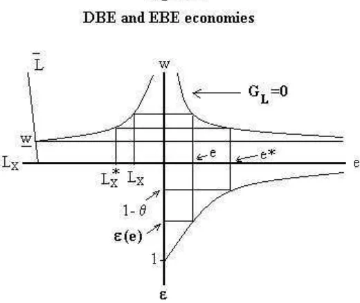
Conditions (91) and (93) constitute the steady state conditions for the domestic goods and labor markets, respectively. Jointly they define the long run equilibrium values of ω and e, as graphed if Figure 2.

The (log) slopes of the two lines are the following:

(96) (ω/e)(de/dω)GP=0 = -

{

}

(97) (ω/e)(de/dω)GL=0 = -{ ε - (1-θ) }-1,

where ε is the elasticity of the export sector product wage w (≡ω/(φe1-θ)) with respect to e along the zero labor gap condition:11

(98) ε≡ -(e/w)/(dw/de) = φeLN’/[LX’+φeLN’ -L’λφ/µW] = [1/ε* + ξ] -1_∈

(0,1),

ε* ≡φeLN’/[LX’+φeLN’] ∈ (0,1),

ξ≡L’λ/[µWρe(-LN’)]>0,

Note that 1/ε is the sum of 1/ε* (the inverse of the analogous elasticity when labor supply is held constant) and ξ. The steady state condition for domestic goods clearly has a negative slope in the e-ω plane but the slope of the labor market balance equation is ambiguous and crucially depends on the sign of ε-(1-θ). As we show in section II.8, under the assumption that our economy is what we call a Domestically Biased Economy in Production relative to Consumption (DBE, for short), the slope is negative. This condition essentially implies that when e increases, the increased demand for labor in the export sector and the lower labor supply do not compensate for the lower demand for labor in the domestic sector, and hence

of the domestic goods balance condition, an increase in λ generates a fall in the steady state value of ω and an increase in the steady state value of e. The opposite occurs when the relation between the slopes is reversed.

From (96) and (97) it follows that the slope of GL=0 is more negative than that of GP=0, because:

(99) (ω/e)(de/dω)GL=0 = -{ θ + (ε-1) }-1 < -1/θ <

< -

{

}

We conclude that the slope of GL=0 is more negative than that of GP=0 if and only if we have a DBE, as we assume, and as depicted in Figure 2. As the figure shows, in a DBE an increase in λ has the effect of increasing the steady state value of e and lowering that of ω.

II.7. The dollar appreciation and its impact on the economy

DBE assumption this increases the steady state value of e and reduces the steady state value of ω. In Figure 3, if the economy was initially at the steady state A, the new steady state is at C (with the steady state inflation rates staying at zero). But what is the impact effect? The definition of e (=E/(ρPN)) guarantees that the increase in ρ makes e fall on impact.

Furthermore, since ω=(W/PN)/eθ and W and PN are predetermined, the rise in ρ makes ω

increase on impact, through the effect of the fall in import prices, which are flexible, on the price level. Hence, the economy moves to point B in Figure 3. It is rather perverse that the impact effects are precisely opposite to the long run effects. And it is especially perverse that a negative shock should have the effect of increasing the real wage!

We can be more precise about the impact effect of the unexpected and temporary strong dollar shock. The effect on ω and e must be such that the product wage in the domestic sector ωeθ maintain its initial value (W/PN)0, and hence must be on a curve as the one

depicted in Figure 3. The (log) slope of this curve at the steady state is –1/θ. But this slope is necessarily between the slopes of GL=0 and GP=0, as (107) proves. This implies that the shock takes the economy to the area where at the initial steady state A there was a negative price gap (GP<0), a negative wage gap (GW<0), and a negative labor gap (GL<0). Because (as we have seen) GP=0 shifts to the right, GL=0 shifts to the left and, therefore, GW=0 also shifts to the left, the economy also has all three gaps negative with the new steady state C. This means that: 1) the supply of labor is greater than the benchmark labor demand (GL<0), 2) the demand for labor is lower than in the benchmark economy (GW<0), and 3) the demand for domestic goods is lower than in the benchmark economy (GP<0). Note that 1) and 2) jointly imply that there is unemployment.

Because the price gap is negative, the domestic price is greater than marginal cost. Hence, firms in the domestic sector start to lower their price, which implies that πN jumps from

zero to a negative value. And the price Phillips curve implies that πN gradually increases,

starting from that negative value. Analogously, because the wage gap is negative, the nominal wage rate is greater than the marginal rate of substitution between leisure and wealth. Hence, households start to lower the wage they set, which makes πW jump from

starting from that negative value. The stability of the steady state equilibrium makes (ω,e) gradually evolve towards C in Figure 3 along a path similar to the one in Figure 1. This means that the economy must traverse a rather lengthy path with deflation, unemployment, and recession before it can reach the new steady state. Even if capital markets were perfect and financed the whole process there would be adverse welfare effects due to the loss of employment, output and domestic income. However, in a global context in which capital flows can suddenly reverse and precipitate a severe crisis the welfare losses can be much more acute, as we develop below.

is further to the northwest than C in Figure 3, as F in Figure 4.12 But this purely

informational shock triggers another, simultaneous, shock. Foreign creditors were willing to finance the debt accumulation generated by the temporary shock, but when the news arrives that the shock is permanent, they are not willing finance the further debt

accumulation that would be needed to get to the new steady state without a devaluation. They prefer to take the haircut on the debt that everyone unanimously expects will result from a sudden stop in financing and the resulting devaluation. Expectations are that if and only if a sudden stop occurs, the government will default, devalue, restructure the debt, assume certain inter-private debts and incur in a major fiscal reform. But since the temporary nature of the dollar appreciation was expected with certainty by everyone, the conditional expectation was devoid of any implication with respect to any further adjustment in consumption. Also, everyone is assumed to believe (rightly) that the

government is not willing or able to make a sufficiently profound direct fiscal reform, in the absence of devaluation and default, that would allow it to avoid further indebtedness. It prefers to devalue, default and restructure its debt, face the realization of contingent

liabilities, and force a combination of fiscal reform and debt forgiveness that is accepted by the population and international creditors, in view of the catastrophic situation. The

devaluation in turn implies a sudden fall in the real wage in our domestically biased economy, one that is certainly greater than the perverse initial increase.

Figure 4 shows the whole story. The initial steady state is at A in both panels. The rise is ρ takes the economy to B on impact, and then gradually along the path that is expected to lead to D. On the left hand panel, the graph shows that λ increases from λ_ to λ0 on impact,

so that the consumption path shifts to the right, which implies lower consumption. On arriving at C, however, the second shock shifts the steady state to F and the devaluation takes the economy to E along a curve as the one depicted in Figure 3. The shift in the steady state is achieved through a new increase in λ to λ+, that again shifts the consumption

12

path to the right. From E, which in the particular case shown in Figure 4 implies

overshooting in e and undershooting in ω, there is again a path that leads to the final steady state F.

ultimately Argentine tax-payers and foreign creditors (through the haircut), will have to pay for the net fiscal cost of the designers of Convertibility’s dogmatic neglect of the huge currency mismatches generated by the banking system.

II.8. The meaning of the DBE assumption

The DBE assumption (that ε>1-θ) played a crucial role above in the characterization of the long run effects on ω and e of an increase in λ. This section explains its exact meaning. Labor demands in the benchmark economy are derived from (26) and (FN’)-1(µPωeθ) (as in

(89)) as decreasing functions of the respective product wages. We may express them as LX(w) and LNn(µPwφe) where w (≡ω/(φe1-θ)) is the export sector product wage and wφe

(≡ωeθ)) is the domestic sector product wage. Labor market clearing in the benchmark economy is hence:

(100) LX(w) + LNn(µPwφe) =L(λwφ/ρµW).

Where labor supply was defined in (92). Equation (100) gives an inverse relation between w and e:

(101) w(e) ( w’<0 ).

The elasticity of w with respect to e is positive and less than unity, as in (98). Note that ε* in (98) is the elasticity of w with respect to e when labor supply is held constant. Hence, ε* is a term related to the structure of labor demand whereas ξ captures the sensitivity of labor supply to w. Also, LX is increasing with e whereas LN is decreasing (because ε<1).

Using (101), the supply functions for goods in the benchmark economy are: (102) yX = FX(L X(w(e))) ≡ yX(e), ( yX’>0 )

yN = FN(LN(w(e)φe))) ≡ yN(e), ( yN’<0 ).

As e increases, labor shifts from the domestic to the export sector.

(100’) LX(ω/(φe1-θ)) + LNn(µPωeθ) =L(λω/ρe1-θµW).

Totally differentiating we obtain the elasticity of ω with respect to e: -(e/ω)(dω/de) = ε - (1-θ).

Hence, the full employment condition in the benchmark economy is such that ω and e vary inversely if and only if ε > 1-θ which, considering (98), is equivalent to 1/ε*+ξ < 1/(1-θ). Note that when labor supply is constant (ξ=0) this condition reduces to ε*>1-θ, which is the necessary and sufficient condition for Lne to be positive:

Lne = (ω/e1-θ) (LN’/ε*)(ε*+θ-1).

From the definition of ε* (in (98)) we see that

ε*>1-θ ⇔ (1-ε*)/ε* = LX’/φeLN’ < θ/(1-θ).

Bearing in mind that w is a function of e and that 1-ε is the elasticity of eφw(e) with respect to e, the last inequality can be expressed as:

(103) (dLX/dlnw)/[-dLN/dln(φew)] < θ/(1-θ).

Thus, ε*>1-θ means that the increase in labor demand in the export sector due to a marginal increase in e (that reduces w), in relation to the marginal reduction in labor demand in the domestic sector (through the increase in eφw), is less than the reduction in imported goods consumption (θ) in relation to the increase in domestic goods consumption (1-θ). More prosaically, an increase in e generates a shift of labor from the domestic to the export sector that is smaller than the shift of consumption from imports to domestic goods. And the stronger condition ε>1-θ essentially means that the sensitivity of labor supply to its argument is not so large as to make 1/ε*+ξ greater than 1/(1-θ).

We now show sufficient conditions for ε* to be a strictly decreasing function of e, in which case the domain of e separates in two segments which respectively define the DBEs and EBEs. Using (101) in the definition of ε* shows that

(104) 1/ε*(e) = h(e) + 1