Keywords:
• cables
• frequency response • power system transients • earth-impedance • ground-return models • skin-effect
Information on the article: received: April 2013, reevaluated: May 2013, accepted: May 2013
Numerical Infinite Series Solution of
the Ground-Return Pollaczek Integral
Solución numérica en series infinitas para la integral
de retorno por tierra de Pollaczek
Uribe-Campos Felipe Alejandro
Departamento de Mecánica EléctricaDivisión de Ingenierías Universidad de Guadalajara,CUCEI
E-mail: fauribe@ieee.org
Abstract
In this paper, the Wedepohl-Wilcox series, proposed for calculating ground-return impedances of buried cables and electromagnetic transients, are analyzed in detail. The origin of this series goes back to the original integral derived by Pollaczek. To enhance the analysis developed here, a numerical comparison between the series, the direct numerical integration of Pollaczek integral, and a proposed hybrid numerical algorithm is presented in this paper. The latter consists on: a) the use of a vector-type efficient algorithm for the converging series for low frequencies, and b) trapezoidal numerical integration for the high frequency range. In addition, and based on the analysis, a criterion for switching between series and direct numerical inte-gration is proposed here.
Resumen
En este artículo se analiza con detalle la serie de Wedepohl-Wilcox, propuesta para calcular impedancias de retorno por tierra de cables subterráneos, así como transito-rios electromagnéticos. El origen de esta serie se remonta a la derivación original de la integral de Pollaczek. Para mejorar el análisis desarrollado aquí se presenta una comparación numérica entre la serie, la integración directa de la integral de Pollac-zek y se presenta un algoritmo híbrido numérico. Este último consiste en: a) el uso eficiente de un algoritmo vectorizado para series convergentes en el rango de baja frecuencia y b) la integración numérica trapezoidal para el rango de alta frecuencia. Adicionalmente, basándose en este análisis, se propone un criterio para switchear entre la solución de la serie y la integración numérica directa.
Descriptores: • cables
• respuesta en frecuencia • transitorios en sistemas de
potencia
• impedancia de tierra
Introduction
One of the most important techniques, over 85 years old, to calculate the influence of the ground-return on aerial and buried electrical conductors was posted by Von F. Pollaczek in June 1926. In this work, Pollaczek presented a set of integral expressions to evaluate the electric field due to an infinite thin filament of current in the presence of an imperfect conducting ground.
Unless, Pollaczek integrals are accurate enough for many power applications, several authors have deve-loped approximate methods and closed-form solu-tions to avoid facing these rapidly increasing oscilla- ting integrals.
One important publication related to this topic was published in 1973 by Wedepohl and Wilcox, in this pu-blication, a complete mathematical model based on the modified Fourier integral for the synthesis of travelling wave phenomena in underground transmission sys-tems was proposed. An important contribution in Wedepohl and Wilcox (1973) is the solution of Pollaczek’s integral through a set of low frequency infi-nite series. To the best author knowledge, an efficient solution of the series has not been implemented nor in-cluded in any commercial software. Besides, it is ar-gued that the series solution is rather complicated and it is better that the impedance is obtained directly from solving the Pollaczek’s integral, numerically.
As a first objective, and inspired on the research in Wedepohl and Wilcox (1973), an efficient numerical im-plementation of the Wedepohl-Wilcox series solution is developed in this paper for calculating ground-return
impedances for underground cables, which can gua-rantee absolute convergence (Kaplan, 1981).
As a second objective, a comparison with four diffe-rent algorithms for solving Pollaczek integral is presen-ted for calculating electromagnetic transients. The first one corresponds to the originally proposed in Wede pohl and Wilcox (1973), i.e., solving the series for low frequencies and using a closed-form solution for the high frequency range. The second algorithm is propo-sed here and corresponds to a hybrid one. This is bapropo-sed on the rapidly converging series for low frequencies, combined with trapezoidal integration of the unexpan-ded integral expression for high frequencies (Wedepohl and Wilcox, 1973). The third and the fourth algorithms consist on trapezoidal numerical integration and Gauss-Kronrod routine, respectively, applied directly to the unexpanded and Pollaczek integral, without using approximating series.
As a third objective, the proposed hybrid algorithm is tested for a wide range of practical application cases on transient analysis. This is achieved by using norma-lized dimensionless variables according to an interpre-tation for underground cables of the application limits reported in (Ametani et al., 2009).
The computational analysis of the studied algo-rithms is presented here regarding accuracy and CPU-time.
Earth-return impedances
Basic relations
The self and mutual earth-return impedance for a qua-si-TEMz (transversal electromagnetic with respect to “z” axis) mode is described by (Figure 1 for reference directions) Wedepohl and Wilcox (1973):
21/ 2 21/ 2 21/ 2
2 2 2 2
( )
2 1/ 2 1/
α α α
α ωm
ω α
π α α α
− + + − − + − + +
∞
−∞
−
= +
+ + +
∫
y h p y h p y h pj x
g j e e e
Z e d
p p
(1a) where α is the dummy variable, w represents the angu-lar frequency (in rad/s), m corresponds to the magnetic permeability (H/m) of the soil, and the complex depth or Skin Effect Layer Thickness (considering displace-ment currents) is given by many authors (Pollaczek, 1926; Wedepohl and Wilcox, 1973; Kaplan, 1981; Ame-tani et al., 2009; Carson, 1926; Uribe et al., 2004; 2000; Dommel, 1986):
1/ ω σ( ωε ε m)
= + o r
p j j (1b)
where σ is the ground resistivity (Ω·m) and ε is the re-lative permittivity (ε0 for the vacuum (F/m) and εr of the
soil).
After the second integral in (1a) is expressed via Bessel functions, where K0 is the Bessel function of zero order, thus (1a) becomes (parameters D and d are shown in Figure1) (Wedepohl and Wilcox, 1973):
[
]
( ) ( / ) ( / ) 2 ωm ω π= o − o + Poll
g j
Z K D p K d p J (2)
where
2
2 3 4
( 2 )
= − +
Poll
J I I I p (3a)
2 2
( ) 1/
2 2
2 α 1/ − + α+ α α
∞
−∞
=
∫
+ ⋅ h y p j xI p e e d (3b)
2 2
( ) 1/
3 α − + α+ α α
∞
=
∫
h y p j xo
I e e d (3c)
2 2
( ) 1/
4 α − + α+ α α
∞
−∞
=
∫
h y p j xI e e d (3d)
According to (3b) and (3d), the solution for I2 and I4 is given by
2 2 2
2 1
2 2 3
2=2(h y+ ) (D/p) +2[(h y+ ) −x ] (D/p)
I K K
D p D p (4a)
2 2
4 2 ( ) (D/p)
+
= jx h y
I K
D (4b)
respectively, where K1 and K2 represent modified Bessel functions of first and second order, respectively. For I3, we have
2 2 /
3 2 2
2 /
2 2 2
2 /
2 2 2
( )/
1 1
( )/
1 [( ) ] +
( ) 1 2 1
1
( ) 2 1 1
1 − − − ∞ + ∞ + = + − + + + − + − + + − − −
∫
∫
∫
Dt p Dt p Dt p h y Dh y D
I h y x te dt
D p
jx h y t e dt
D p t
x h y t e dt
D p t
(4c)
The first part of the integral in (4c) is easily evaluated by traditional integration; the second part corresponds to K2(D/p). In Wedepohl and Wilcox (1973), it is
propo-sed that the third part of (4c) be evaluated by series ex-pansion of the exponential function and then integrated term-by-term to give Sser(D/p, |x|, 1), with ℓ = h + y.
That is
[
]
2 2 ( )/ 3 4 2 2 2 2 2[( ) ] 1 ( ) /
( ) ( / ) ( ) , , − + + − = + + + + + + + +
h y p
ser
h y x
I h y p e
D
jx h y K D p D
x h y S D x
p D p
(4d)
The series term Sser from (4d) is further analyzed in the
following sections.
Wedepohl-Wilcox series
Despite some typographical errors in Wedepohl and Wilcox (1973) regarding the converging series, these can be split up into the following four types of terms:
1 2 3 4
( , , ) = + + +
ser D
S x S S S S
p (5)
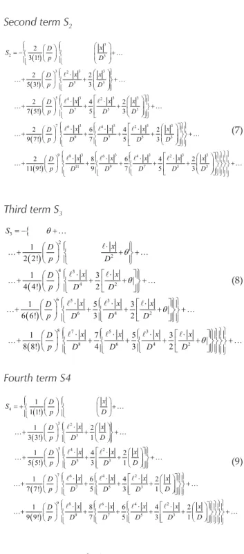
S1 to S4 are displayed here differently than in Wedepohl and Wilcox (1973) for better clarity of programming im-plementation, as shown in (6). For instance, an analysis of S1, given by (6a), reveals that the leading terms
and k = 2, 3,...
can be stored into two separate vectors and used whe-never is required. In addition, it can be observed in (6)-(9) the nesting nature of the remaining terms.
It is noted that the aforementioned leading terms are frequency dependent whilst the nested terms de-pend only on the geometry of the cable system.
First term S1
(6a) 2 , k D p + ( ) ( ) ( ) 1 2 3 2 4 2 3 3 4 3
6 4 2
3 3 3
6 5 3
8 6 4 2
1 1
2 2! 2
1 3 1
3 4! 4 2
1 5 3 1
4 6! 6 4 2
θ θ θ θ ⋅ = − + ⋅ ⋅ + + − + ⋅ ⋅ ⋅ + + + − + ⋅ ⋅ ⋅ ⋅ + + + + − x S D x x D
p D D
x x x
D
p D D D
x x x x
D
p D D D D
( )
3 3 3 3
8 7 5 3
10 8 6 4 2
1 7 5 3 1
5 8! 8 6 4 2 θ
+ ⋅ ⋅ ⋅ ⋅ ⋅ + + + + + − +
D x x x x x
p D D D D D
1 ( 2)!
Second term S2
(7)
Third term S3
{ ( ) ( ) ( ) ( ) 3 2 2 4 3 4 2
6 5 3
6 4 2
8 7 5 3
8 6 4
1 2 2!
1 3
4 4! 2
1 5 3
6 6! 3 2
1 7 5 3
8 8! 4 3 2
θ θ θ θ = − + ⋅ + + + ⋅ ⋅ + + + + ⋅ ⋅ ⋅ + + + + + ⋅ ⋅ ⋅ + + + + S x D p D x x D
p D D
x x x
D
p D D D
x x x
D
p D D D 2 θ
⋅ + +
x
D
(8)
Fourth term S4
( ) ( ) ( ) ( ) 4 3 2 3
5 4 2
5 3
7 6 4 2
7 5 3
1 1 1!
1 2
3 3! 1
1 4 2
5 5! 3 1
1 6 4 2
7 7! 5 3 1
= + + ⋅ + + + ⋅ ⋅ + + + + ⋅ ⋅ ⋅ + + + + x D S p D x x D
p D D
x x x
D
p D D D
x x x x
D
p D D D D
( )
9 8 6 4 2
9 7 5 3
1 8 6 4 2
9 9! 7 5 3 1
+ ⋅ ⋅ ⋅ ⋅ + + + + + +
D x x x x x
p D D D D D
(9)
Convergence analysis
Series versus numerical integration
Consider the three cable application case reported in Wedepohl and Wilcox (1973) and reproduced here in Figure 2. For this case, the frequency range has been uniformly sampled from 1Hz to 10MHz by using 100 points.
Figure 2. Underground cable transmission system, taken from Wedepohl and Wilcox (1973)
As a first evaluation, we use the series proposed by Wedepohl-Wilcox, Sser, given by (5). The second
evalua-tion corresponds to the trapezoidal-based numerical integration of the third integral in (4c), labeled Sint. A
step equal to 10–4 has been used for calculating S
int. The
behavior of both evaluations is presented in Figure 3a. In this figure, the real and complex components of Sint
are presented in black continuous dotted line. As for the Sser, the number of terms has been varied and the
corres-ponding result is shown in the gray dashed line. From the results in Figure 3a, it can be noticed that the first four terms of each Sn, n = 1…, 4, give a fairly good
agree-ment compared to Sint. Further evaluations including
more than four terms did not change meaningfully the results given by Sser. This obeys to the theory of
conver-gence of a series around a given point (Kaplan, 1981).
Ratio test
In addition, the uniform convergence of the sequence of partial sums (or series solution Sn) has been calculated
by using the following ratio test (Kaplan, 1981), for n = 1, 2, 3, and 4
1
lim + < 1
→∞ k k n k n S S (10)
The results of evaluating (10) are shown in Figure 3b. From this numerical analysis, one can observe the smooth behavior of the four sets of curves Sn when
ap-proximating Sser which indicates a uniform convergence
feature, as defined in (Kaplan, 1981).
Proposed hybrid algorithm
From Figure 3a it can be seen that all four terms of the series give accurate results, at very low computational ( ) ( ) ( ) ( ) 3 2 3 3 3 3 2 5 3
3 3 3
5 4 2
7 5 3
3 3 3
7 6 4 2
9 7 5
2 3 1!
2 2
5 3! 3
2 4 2
7 5! 5 3
2 6 4 2
9 7! 7 5
= − + ⋅ + + + ⋅ ⋅ + + + + ⋅ ⋅ ⋅ + + + + x D S p D x x D
p D D
x x x
D
p D D D
x x x
D
p D D D
( )
3 3
3 3 3 3 3
9 8 6 4 2
11 9 7 5 3
3
2 8 6 4 2
11 9! 9 7 5 3
+ ⋅ ⋅ ⋅ ⋅ + + + + + + x D
x x x x x
D
expenses, up to D/|p| ≈ 2. Therefore, it is proposed here to use this number as a criterion for a hybrid algorithm that switches between series and numerical integration. This criterion contrasts to the one proposed in Wedepo-hl and Wilcox (1973) where D/|p| = 1/4 is used to switch between series and a closed form solution of (2). Fur-thermore, in the proposed hybrid algorithm, the displa-cement current has also been accounted for, as indicated in (1b).
a)
b)
Figure 3. Series convergence test, a)comparison between series solution and trapezoidal
integration regarding the number of terms, b)ratio test for convergence (Kaplan, 1981)
The main numerical characteristics of the results that have been obtained for the particular underground ca-ble system configuration in Figure 2 are general. Thus, it can also be extended to a broad range of cable confi-gurations as explained in the following section.
Broad range algorithmic solution
It should be mentioned here that the earth-return impe-dance, given by (1) has been traditionally handled by using true variables. That is, specific physical and
geo-metrical parameters and continuous complex frequen-cy variables are usually involved to calculate the earth return impedance of the system. This consideration is perfectly valid when simulating a transient in that spe-cific system.
Nevertheless, a simple change of variables, as pro-posed here, leads to a wide range representation of the earth return impedance. The wide range formulation encloses the majority of practical cases and can be also used as benchmark for alternative solution methods.
Consider the following normalized dimensionless parameter definitions, which are graphically represen-ted in Figure 4 (Carson, 1926; Uribe, 2004)
, and
x
= +h
=c
= −+ +
y h x y h
p y h y h (11a)
After some mathematical manipulations, one obtains the wide-range representation of (2) as (Uribe, 2004)
2 2 2
0 0
2π ( x c h ) ( x 1 h ) ( , )x h ωm
= ⋅ ⋅ + − ⋅ + +
Ground 0 Poll
Z j K j K j J
(11b)
where now the term JPoll has been transformed into the
following normalized parameter version of the Pollac-zek integral (Carson, 1926; Uribe, 2004)
(
)
(
)
2
2 0
exp
, 2 x cos
x h x h
∞
− +
= ⋅
+ +
∫
Pollu j
J u du
u u j (11c)
In obtaining (11c), the change of variable α = u/|p| has been applied also to (1a).
Moreover, the transformation to normalized para-meters is of general applicability. For instance, consider the following closed-form expression derived by Wede-pohl-Wilcox from the series expansion (Wedepohl and Wilcox, 1973)
(
)
(
)
0 1 2
2
ωm γ
π
+
= ⋅ − + −
Ground
h y j
Z log d 2p
2 3p (11d)
In the normalized parameter form, (11d) becomes now a function of x, c, and h, as follows (Uribe, 2004)
(
2 2)
0
2 1
2
π γ x c h x
ωm
= ⋅ − ⋅ + + − ⋅
Ground 2
Z j log j 2 j
3
Figure 4. Dimensionless normalized vector relations between parameters as described first by Carson’s ground-wave propagation theory (Carson, 1926)
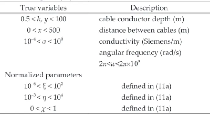
The range for both true and normalized variables is presented in Table 1, following the recommendations from (Ametani et al., 2009). Although the numerical so-lution of (11c) can be computed, one can take the fast hybrid solution in true variables, as described in the last section “proposed hybrid algorithm”. Then, the re-sult can be transformed into dimensionless variables by using (11a).
Table 1. Ranges of physical and normalized variables
True variables Description 0.5 < h, y < 100 cable conductor depth (m)
0 < x < 500 distance between cables (m)
10−4 < σ < 100 conductivity (Siemens/m)
angular frequency (rad/s)
2π<w<2π×109
Normalized parameters
10−6 < ξ < 102 defined in (11a)
10−3 < η < 104 defined in (11a)
0 < χ < 1 defined in (11a)
Figure 5 depicts the numerical solution of JPoll(x,h), given by (11c). This solution was obtained with the hy-brid algorithm where 100 samples for x and 10 sam-ples for h have been used. The results obtained by the Wedepohl-Wilcox algorithm, by trapezoidal
integra-tion, and by the Gauss-Kronrod algorithm can be seen in Appendix A.
For the numerical analysis in the next section, the hy-brid algorithm is taken as basis. Firstly, it has a strong fun-dament on the numerical analysis presented in section “series versus numerical integration”, specifically for the switching criterions. Secondly, it does not show numerical oscillations as other methods (Figure 11, Appendix A).
Computational analysis
The computational performance of the aforementioned methodologies for obtaining the wide range solution curves (as shown in Figure 5) is presented in Table 2. The first one corresponds to the trapezoidal integration applied to the third integral in (4c). The second one is the hybrid algorithm proposed here which uses the convergent series from (5) combined with trapezoidal integration on (4c). The third one uses the Wedepohl-Wilcox algorithm using the convergent series at the low frequency range and formula (11d) or (11e) for the high frequency one (Wedepohl and Wilcox, 1973). Finally, the fourth one consists on a widely used method, i.e., Gauss-Kronrod, directly to the wide range formulation (11c) using the default absolute tolerance of 10–10 (using double precision format).
Table 2 resumes the rms-error (calculated in a classi-cal form (Kaplan, 1981) and the computational times required by the four methods. Only the results for three different values of h, chosen from the curves in Figure 5, are shown in Table 2. To obtain the results in Table 2, Matlab® v7.8 on a 2.4GHz processor with 8GHz RAM was used.
From Table 2 it can be observed that the computatio-nal time by the Gauss-Kronrod method is larger than the rest of the methods (much larger for η10), as expec-ted. The Wedepohl-Wilcox solution takes CPU times
a) b)
Figure 5. Wide range solution of JPoll(x ,h)calculated here with the proposedhybrid algorithm, a)real component,
comparable to trapezoidal and hybrid methods; howe-ver, its rms-error increases for larger values of h. This is perhaps due to the “weak” criterion for switching bet-ween the series and the closed-formula.
Transient
A transient calculation of the underground cable sys-tem of 5km length, shown in Figure 2, is presented in the following. The open circuit voltage and the short circuit current responses are both calculated through the inverse Numerical Laplace Transform (cable data are available in Appendix B) (Uribe et al., 2000).
A unit step voltage is injected to the core of cable 1 at the sending end of the underground cable system. The voltages at the receiving end are shown in Figure 6a for the energized core, while Figure 6b presents the induced voltages for cores 3 and 5, and sheaths 2, 4 and 6.
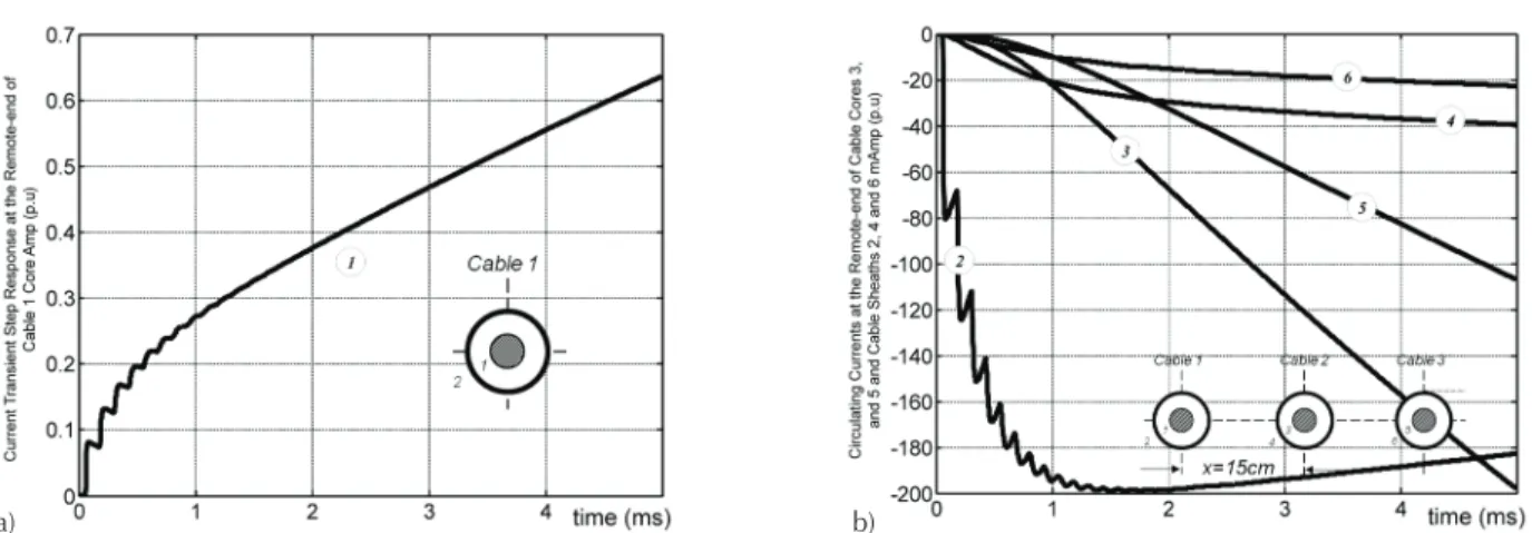
The currents at the receiving end are depicted in Fi-gure 7a for the energized core 1 and in FiFi-gure 7b for the circulating currents.
Each core and sheath conductor of the cable system is coupled with each other through four different ground-return loops.
It should be mentioned here that, when the core of cable 1 is energized, the magnitude of the induced vol-tages and circulating currents for the presented test ca-ses, become naturally smaller as the ground loop distances increases. In these cases, the accuracy of the ground-return impedance calculation becomes impor-tant to identify electromagnetic couplings or interferen-ce phenomena between underground and overhead transmission or communication systems (Carson, 1926; Dommel, 1986).
Hence, the ground return modeling would directly impact on the estimated voltage or current waveform
Table 2. Cpu times and rms error
Trapezoidal rule on (4c)
Test methodology Hybrid algorithm
on (4c) and (5) Wedepohl-Wilcox algorithm (5) and (11d) Direct Gauss-Kronrod on (11c)
h1
CPU time
(Sec) 0.075400400 0.06800050 0.09360059 0.358802
rms error 0.000010414 (base) 0.03823930 0.000003
h5
CPU time
(Sec) 0.079000500 0.07600050 0.0780005 0.3900024
rms error 0.004299822 (base) 0.0444786 0.0006413
h10
CPU time
(Sec) 0.075400400 0.06360060 0.0936006 6.3024403
rms error 0.000000929 (base) 0.2089789 0.0071932
a) b)
magnitude responses and on their respective phase be-havior.
The transient response corresponding to Figures 6 and 7 have been also obtained with: Gauss-Kronrod di-rect numerical integration on (11c), the EMTP methodo-logy (Dommel, 1986) and the Wedepohl-Wilcox (1973) derived formula (11d).
In the EMTP methodology the evaluation of the Po-llaczek integral JPoll in (2) is replaced by the evaluation
of Carson’s integral (Dommel, 1986).
Figure 8a depicts the relative differences for the indu-ced voltage of the loops formed between core-1 on core-5 (circle 5 marker) and on sheath-6 (circle 6 marker), calcu-lated with the aforementioned methods. Figure 8b pre-sents the relative differences for their corresponding circulating currents.
As a second application case, consider again the ca-ble transmission system from Figure 2 (Wedepohl and Wilcox, 1973), but now configured with a separation distance between cables equal to x = 5m.
The calculated induced voltages for this second stu-dy case are shown in Figure 9a, while the circulating currents are presented in Figure 9b. The corresponding relative differences are shown in Figure 10.
The comparison of Figures 6b and 9a shows that, the greater the distance between cables the lower the indu-ced voltage magnitude, as expected. For this case, the relative differences for the longer formed loops bet-ween -core conductor 1 and core conductor 6 and sheath conductor 6 (as shown in Figures 8a and 10a) are more than three times bigger. This confirms that ground return models are highly sensitive on transient applica-tions to the normalized parameters in (11a).
A distinct behavior is presented on the circulating currents in the sheath conductor 2 of the energized ca-ble 1. The greater the distance between caca-bles the grea-ter the magnitude of the current. The relative differences shown in Figures 8b and10b indicate a poor performan-ce at low frequencies of the ground return models for this example.
a) b)
Figure 8. Relative differences for transient wave-form responses formed between loops cable core-1, cable core-5 and cable sheath-6, a) induced voltages, b) circulating currents
a) b)
Conclusions
The Wedepohl-Wilcox original infinite series formula-tion to approximate the ground return impedance, as given by Pollaczek, has been implemented and numeri-cally analyzed in this paper.
An alternative new hybrid method, applicable for both real and wide range dimensionless variables, has also been proposed and also analyzed in this paper. Since the proposed hybrid algorithm can be established for a wide range of physical and geometrical variables, it can be used to define any practical application ranges for approximate formulas and also to assess any other numerical methods (based on quadrature, infinite se-ries, conformal mapping, numerical optimization, etc.) for improving accuracy on transient calculations.
For many years several algorithms to calculate the ground impedance have also been implemented and applied to a transient analysis. From the obtained re-sults, it has been noticed that a precise calculation of such impedance is needed to obtain accurate and relia-ble time domain transient responses.
Appendix A
The wide range approximate solutions of Pollaczek’s integral calculated via the Wedepohl-Wilcox algorithm, trapezoidal integration, and Gauss-Kronrod algorithm, are depicted in Figure 11. There are some numerical os-cillations, that are more noticeable in the real com-ponent case of the η10 curve (its value is tabulated in
a) b)
Figure 9. Second study case transient. Step-responses at the receiving end of the cable system, a) induced voltages, b) circulating currents
a) b)
Figure 5), when applying the Gauss-Kronrod algorithm in the following range 10-4 < x < 100.
Appendix B
Cable design specifications for the paper transient application cases are depicted in Figure 12.
References
Ametani A., Yoneda T., Baba Y., Nagaoka N. An Investigation of Earth-Return Impedance Between Overhead and Underground Conductors and its Applications. IEEE Transactions on
Electro-magnetic Compatibility, volume 51 (issue 3), August 2009: 860-867.
Carson J.R. Wave Propagation in Overhead Wires with Ground Return. Bell Systems Tech. J., 1926: 539-554.
Dommel W. Electromagnetic Transients Program Reference
Ma-nual (EMTP Theory Book), Prepared for Bonneville Power Ad -ministration, P.O. Box 3621, Portland, Ore., 97208, USA, 1986.
Kaplan W. Advanced Mathematics for Engineers, chapter 2, Addison Wesley, 1981.
Pollaczek F. Über das Feld einer unendlich langen wechsel
strom-durchflossenen Einfachleitung. Electrishe Nachrichten Technik,
volume 3 (issue 9), 1926: 339-360.
Uribe F.A., Naredo J.L., Moreno P., Guardado L. Algorithmic Evalua -tion of Underground Cable Earth Impedances. IEEE Transactions
on Power Delivery, volume 19 (issue 1), January 2004: 316-322.
Uribe F.A., Naredo J.L., Moreno P., Guardado L. Electromagnetic
Transients in Underground Transmission Systems Through the
Numerical Laplace Transform, International Journal of Electrical
Power & Energy Systems, Elsevier Science Ltd, September 2000.
Wedepohl L.M. and Wilcox D.J. Transient Analysis of Under -ground Power-Transmission Systems. Proc. IEE, volume 120
(issue 2), february 1973: 253-260.
Citation for this article:
Chicago citation style
Uribe-Campos, Felipe Alejandro. Numerical Infinite Series Solu-tion of the Ground-Return Pollaczek Integral. Ingeniería Investiga-ción y Tecnología, XVI, 01 (2015): 49-58.
ISO 690 citation style
Uribe-Campos F.A. Numerical Infinite Series Solution of the Ground-Return Pollaczek Integral. Ingeniería Investigación y Tec-nología, volume XVI (issue 1), January-March 2015: 49-58.
About the author
Felipe Alejandro Uribe-Campos. Received the B.Sc. and M.Sc. degrees of Electrical Engineering, both from the State
University of Guadalajara, in 1994 and 1998, respectively. During 2001 he was a visiting researcher at the Univer -sity of British Columbia, B.C. Canada. In 2002 he received the Dr. Sc. degree of Electrical Engineering from the Center for Research and Advanced Studies of Mexico. The dissertation was awarded with the Arturo Rosen-blueth prize. From 2003 to 2006 he was a full professor with the Electrical Graduate Program at the State
Univer-sity of Nuevo Leon, México. In May 2006, Dr. Uribe joined the Electrical Engineering Graduate Program at the State University of Guadalajara, México, where he is a full time researcher. Since 2004, he is a member of the National System of Researchers of Mexico (SNI). His primary interest is the electromagnetic simulation of biolo -gical tissues for early cancer detection, and power system harmonic and transient analysis.
Figure 12. Original cable data for the electromagnetic transient calculation example, taken from Wedepohl and Wilcox (1973)
Figure 11. Wide range solution of JApprox (x,h)
calculated with approximate methodologies, a) real
component, b) imaginary component