A low-order mixed finite element method for a class of
quasi-Newtonian Stokes flows.
Part II: a posteriori error analysis
Gabriel N. Gatica
a,*, Mar
ıa Gonz
alez
b, Salim Meddahi
c aGI2MA, Departamento de Ingenierıa Matematica, Universidad de Concepcion, Casilla 160-C, Concepcion, ChilebDepartamento de Matem
aticas, Universidade da Coru~na, 15071 A Coru~na, Spain
cDepartamento de Matem
aticas, Universidad de Oviedo, Calvo Sotelo s/n, 33007 Oviedo, Spain
Received 9 December 2002; received in revised form 8 September 2003; accepted 10 November 2003
Abstract
This is the second part of a work dealing with a low-order mixed finite element method for a class of nonlinear Stokes models arising in quasi-Newtonian fluids. In the first part we showed that the resulting variational formulation is given by a twofold saddle point operator equation, and that the corresponding Galerkin scheme becomes well posed with piecewise constant functions and Raviart–Thomas spaces of lowest order as the associated finite element sub-spaces. In this paper we develop a Bank–Weiser type a posteriori error analysis yielding a reliable estimate and propose the corresponding adaptive algorithm to compute the mixed finite element solutions. Several numerical results illus-trating the efficiency of the method are also provided.
Ó 2003 Elsevier B.V. All rights reserved.
AMS:65N30; 65N22; 65N15; 76D07; 76M10
Keywords:Mixed finite element method; Twofold saddle point formulation; A posteriori error analysis
1. Introduction
We first recall from [5] the boundary value problem of interest. Indeed, letXbe a bounded and simply connected domain in R2 with Lipschitz-continuous boundary C. Our goal is to determine the velocity
u:¼ ðu1;u2Þ t
and the pressurepof a nonlinear Stokes fluid occupying the region Xunder the action of an external force. More precisely, givenf2 ½L2ðXÞ2
andg2 ½H1=2ðCÞ2
, we look forðu;pÞin appropriate spaces such that
*Corresponding author.
E-mail addresses: [email protected] (G.N. Gatica), [email protected] (M. Gonzalez), [email protected] (S. Meddahi).
0045-7825/$ - see front matter Ó 2003 Elsevier B.V. All rights reserved. doi:10.1016/j.cma.2003.11.008
Comput. Methods Appl. Mech. Engrg. 193 (2004) 893–911
divðwðjrujÞrupIÞ ¼f inX;
divðuÞ ¼0 inX; andu¼g on C; ð1:1Þ
wheredivand div are the usual vector and scalar divergence operators,ruis the tensor gradient ofu,j jis the euclidean norm of R2, Iis the identity matrix of R22, and w:Rþ !Rþ is the nonlinear kinematic viscosity function of the fluid. We remark that g2 ½H1=2ðCÞ2
must satisfy the compatibility condition
R
Cgmds¼0, wheremis the unit outward normal toC.
We now letw:R22!R22be the tensor defined bywðrÞ:¼ ðwðjrjÞrijÞfor allr2R22. Then, the mixed variational formulation of (1.1), as deduced in [5], which introducesr:¼wðruÞ pIandt:¼ ruas further unknowns, reads as follows: Findðt;ðr;pÞ;ðu;nÞÞ 2X1M1M such that
½A1ðtÞ;s þ ½B1ðsÞ;ðr;pÞ ¼0;
½B1ðtÞ;ðs;qÞ þ ½Bðs;qÞ;ðu;nÞ ¼ ½G;ðs;qÞ;
½Bðr;pÞ;ðv;gÞ ¼ ½F;ðv;gÞ;
ð1:2Þ
for allðs;ðs;qÞ;ðv;gÞÞ 2X1M1M, whereX1:¼ ½L2ðXÞ 22
,M1:¼Hðdiv;XÞ L2ðXÞ,M :¼ ½L2ðXÞ 2
R, and the operatorsA1:X1!X10,B1:X1!M10, andB:M1!M0, and the functionalsðG;FÞ 2M10M0, are defined as follows:
½A1ðrÞ;s:¼
Z
X
wðrÞ:sdx; ½B1ðrÞ;ðs;qÞ:¼
Z
X
s:rdx
Z
X
qtrðrÞdx; ð1:3Þ
½Bðs;qÞ;ðv;gÞ:¼
Z
X
vdivsdxþg
Z
X
trðsÞdx; ð1:4Þ
½G;ðs;qÞ:¼ hsm;giC and ½F;ðv;gÞ:¼
Z
X
fvdx; ð1:5Þ
for allr,s2X1,ðs;qÞ 2M1, andðv;gÞ 2M.
Hereafter,½; stands for the duality pairing induced by the corresponding operators and functionals,
h;iC denotes the duality pairing of½H1=2ðCÞ2
and½H1=2ðCÞ2
with respect to the½L2ðCÞ2
-inner product, and Hðdiv;XÞ is the space of tensors s2 ½L2ðXÞ22
satisfying divðsÞ 2 ½L2ðXÞ2
. It is well known that
Hðdiv;XÞ, provided with the inner product hf;siHðdiv;XÞ:¼ hf;si½L2ðXÞ22þ hdivf;divsi½L2ðXÞ2, is a Hilbert
space, where h;i½L2ðXÞ22 and h;i½L2ðXÞ2 stand for the usual inner products of ½L2ðXÞ22 and ½L2ðXÞ2,
respectively. The other notations to be used in this paper are the same as those employed in [5].
In order to define the corresponding mixed finite element scheme, we now assume for simplicity thatCis a polygonal curve, and letfThgh>0be a regular family of triangulations ofXby trianglesT of diameterhT such that h:¼maxfhT :T2Thg and X¼ [fT :T 2Thg. For each T 2Th we let RT0ðTÞ be the local
Raviart–Thomas space of order zero, that is RT0ðTÞ:¼span 1 0 ;
0 1 ;
x1
x2
, where x1
x2 is a
generic vector ofR2. In addition, given a nonnegative integerkand a subsetSofR2, we letPkðSÞbe the space of polynomials defined onSof degree 6k.
Then we introduce the following finite element subspaces:
X1;h:¼ s2 ½L2ðXÞ22:sjT 2 ½P0ðTÞ228T 2Th
n o
;
M1r;h:¼ s:¼ ðsijÞ 2Hðdiv;XÞ:ðsi1si2Þ t
jT 2RT0ðTÞ 8i2 f1;2g;8T 2Th
;
M1p;h:¼ fq2L2ðXÞ:qjT 2P0ðTÞ 8T 2Thg;
M1;h:¼M1r;hM p 1;h;
Mu
h :¼ fv2 ½L 2ðXÞ2
:vjT 2 ½P0ðTÞ 2
8T 2Thg; and
Mh:¼MhuR:
Hence, the Galerkin scheme associated with (1.2) reads: Find ðth;ðrh;phÞ;ðuh;nhÞÞ 2X1;hM1;hMh such that
½A1ðthÞ;sh þ ½B1ðshÞ;ðrh;phÞ ¼0;
½B1ðthÞ;ðsh;qhÞ þ ½Bðsh;qhÞ;ðuh;nhÞ ¼ ½G;ðsh;qhÞ;
½Bðrh;phÞ;ðvh;ghÞ ¼ ½F;ðvh;ghÞ;
ð1:6Þ
for allðsh;ðsh;qhÞ;ðvh;ghÞÞ 2X1;hM1;hMh.
In [5] we proved that, under suitable assumptions on the nonlinear kinematic viscosity functionw(see Eqs. (1.2) and (1.3) in [5]), the continuous formulation (1.2) and the Galerkin scheme (1.6) are well posed. In addition, we derived there the associated a priori error analysis and the corresponding rate of conver-gence. We refer to Theorems 2.4, 3.1, and 3.2 in [5] for details.
On the other hand, we recall that the application of adaptive algorithms, based on a posteriori error estimates, usually guarantees the quasi-optimal rate of convergence of the finite element solution to boundary value problems. In addition, this adaptivity is specially necessary for nonlinear problems where no a priori hints on how to build suitable meshes are available. To this respect, we have shown recently that the combination of the usual Bank–Weiser approach from [1] with the analysis from [3,4] allows to derive fully explicit and reliable a posteriori error estimates for the dual-mixed variational formulations (showing a two-fold saddle point structure) of some linear and nonlinear problems (see, e.g. [2,6,7]). However, no a pos-teriori error analysis has been developed yet for the nonlinear Stokes problems studied in [5]. Therefore, as a natural continuation of our results in [5], in the present paper we apply the Bank–Weiser type a posteriori error analysis mentioned above to derive reliable estimates for the mixed finite element scheme (1.6). The rest of this work is organized as follows. In Section 2 we collect some basic results on Sobolev spaces and state the main result of this paper. The proof of our a posteriori estimate, which makes use of the Ritz projection of the error, is provided in Section 3. In Section 4 we prove thequasi-efficiencyof the estimator and discuss on suitable choices for the auxiliary functions needed for its computation. Finally, several numerical results illustrating the good performance of the adaptive algorithm are reported in Section 5.
2. The main result
2.1. Preliminaries
Let us first introduce some notations. GivenT 2Th, we letEðTÞbe the set of its edges, and letEhbe the set of all edges of the triangulation Th. In particular, we put EhðCÞ:¼ fe2Eh:eCg. Also,h;iHðdiv;TÞ denotes the inner product ofHðdiv;TÞ, andmT stands for the unit outward normal tooT.
In addition, given a polygonal domainSR2ands2 ð1;1Þ, the Sobolev spaceW1;sðSÞis the space of functionsv2LsðSÞsuch that the first order distributional derivatives ofvare functions ofLsðSÞ(see [8]). It is well known thatW1;sðSÞendowed with the norm
kvkW1;sðSÞ:¼ kvk
s LsðSÞ
þ krvks½LsðSÞ2
1=s
is a Banach space. The trace Theorem ensures that there exists a linear continuous map c:W1;sðSÞ 7!
LsðoSÞsuch thatcv¼vj
oSfor eachv2W1;sðSÞ \CðSÞ. It is usual to denoteW11=s;sðoSÞ:¼cðW1;sðSÞÞ which is a strict subspace ofLsðoSÞ(see [8]). We also recall, by virtue of a Sobolev imbedding theorem, that
W1;sðSÞ CðSÞifs>2.
We now take in particular S:¼T 2Th. Then when s¼2 we use the standard notation and write
H1=2ðoTÞinstead ofW1=2;2ðoTÞ. The fractional Sobolev spacesH1=2ðoTÞmay be equivalently defined by the completion of the space of indefinitely differentiable functions in the norm:
kvkH1=2ðoTÞ¼ kvk
2 L2ðoTÞ
þ jvj2H1=2ðoTÞ
1=2 ;
where
jvj2H1=2ðoTÞ:¼
Z
oT
Z
oT
jvðxÞ vðyÞj2 jxyj2 dsxdsy:
Let us now consider an edge e2EðTÞ. Then, H1
0ðeÞ stands for the closure in H1ðeÞ of the space of indefinitely differentiable functions with compact support in e. Finally, we recall that the interpolation space with index 1/2 betweenH1
0ðeÞandL2ðeÞisH 1=2
00 ðeÞ(cf. [8]), and its norm is given by
kvkH1=2 00ðeÞ
¼ jvj2H1=2ðeÞ
þ
Z
e
v2ðxÞ
jxa1j dsxþ
Z
e
v2ðxÞ
jxa2j dsx
1=2 ;
where a1 and a2 are the end points of the edgee. The spaceH 1=2
00 ðeÞmay be alternatively defined as the subspace of functions inH1=2ðeÞwhose extensions by zero to the rest ofoT belong toH1=2ðoTÞ.
We will also need in the sequel the dual space ofH1=2ðoTÞdenoted hereH1=2ðoTÞ. It is important to retain that the restriction of an element inH1=2ðoTÞoveredoes not belong in general toH1=2ðeÞ, but to the dual ofH001=2ðeÞ, usually denoted by H001=2ðeÞ, and which is larger thanH1=2ðeÞ. According to this, in what follows we denote byh;iethe duality pairing between ½H001=2ðeÞ2 and½H001=2ðeÞ2with respect to the
½L2ðeÞ2-inner product. Further, we also denote by h;i
oT the duality pairing between ½H1=2ðoTÞ 2
and
½H1=2ðoTÞ2
with respect to the ½L2ðoTÞ2
-inner product.
2.2. The a posteriori error estimate
The main result of this paper is stated as follows.
Theorem 2.1. Let~t:¼ ðt;ðr;pÞ;ðu;nÞÞ 2X1M1M and~th:¼ ðth;ðrh;phÞ;ðuh;nhÞÞ 2X1;hM1;hMh be the solutions of the continuous and Galerkin formulations (1.2) and (1.6), respectively. Assume there exists
s>2 such that g2 ½H1=2ðCÞ \W11=s;sðCÞ2
and let uh be a function in ½H1ðXÞ \W1;sðXÞ 2
such that uhðxÞ ¼gðxÞfor each vertexxofThlying onC. In addition, letrT^ 2Hðdiv;TÞbe the unique solution of the local problem
h^rT;siHðdiv;TÞ¼Fh;TðsÞ 8s2Hðdiv;TÞ; ð2:1Þ
where Fh;T 2Hðdiv;TÞ0 is defined by
Fh;TðsÞ:¼
Z
T
s:thdxþ
Z
T
uhdivsdxnh
Z
T
trðsÞdx hsmT;uhioTþ
X
e2EðTÞ\EhðCÞ
hsmT;uhgie:
Then,there existsC>0,independent ofh, such that
k~t~thk X1M1M
6Ch:¼C X
T2Th
h2T
( )1=2
; ð2:2Þ
where for each triangleT 2Th we define
h2T :¼ k^rTk2Hðdiv;TÞþ krhwðthÞ þphIk 2
½L2ðTÞ22þ kfþdivrhk
2
½L2ðTÞ2þ ktrðthÞk 2
L2ðTÞ: ð2:3Þ
Further,let u~h be a function in½L2ðXÞ 2
such thatu~h;T :¼u~hjT 2 ½H 1ðTÞ2
for each T 2Th. Then, there existsC~ >0,independent ofh,such that
k~t~thk
X1M1M6 ~
C~h:¼C~ X
T2Th ~
h2T
( )1=2
; ð2:4Þ
where
~
h2T :¼ kth r~uh;Tk 2
½L2ðTÞ22þ kuhu~h;Tk2
½L2ðTÞ2þh2Tjnhj2þ
X
e2EðTÞ\EhðCÞ
kuhgk 2 ½H001=2ðeÞ2
þ kuhu~h;Tk 2
½H1=2ðoTÞ2þ krhwðthÞ þphIk2
½L2ðTÞ22þ kfþdivrhk2
½L2ðTÞ2þ ktrðthÞk2L2ðTÞ: ð2:5Þ
In particular,if we take u~h¼uh,then (2.4) becomes
k~t~thk X1M1M
6C^^h:¼C^ X T2Th ^
h2T
( )1=2
; ð2:6Þ
where
^
h2T :¼ kth ruhk 2
½L2ðTÞ22þ kuhuhk½L22ðTÞ2þh2Tjnhj2þ
X
e2EðTÞ\EhðCÞ
kuhgk 2 ½H001=2ðeÞ2
þ krhwðthÞ þphIk 2
½L2ðTÞ22þ kfþdivrhk
2
½L2ðTÞ2þ ktrðthÞk 2
L2ðTÞ: ð2:7Þ
The proof of Theorem 2.1 is given in the following section. We just remark here that the hypotheses ong
anduhguarantee, by virtue of the Sobolev imbedding theorems, thatganduhare both continuous and that
ðguhÞje2 ½H 1=2 00 ðeÞ
2
for eache2EhðCÞ.
3. The proof of the main result
The proof itself is provided below in Section 3.2. For this purpose, we need to introduce first the Ritz projection of the error.
3.1. Ritz projection of the error
LetX :¼X1M1and introduce the nonlinear saddle point operator A:X !X0given by the first two rows and two columns of (1.2), that is
½Aðt;ðr;pÞÞ;ðs;ðs;qÞÞ:¼ ½A1ðtÞ;s þ ½B1ðsÞ;ðr;pÞ þ ½B1ðtÞ;ðs;qÞ; for allðt;ðr;pÞÞ,ðs;ðs;qÞÞ 2X.
Then we define the Ritz projection of the error, with respect to the inner product of X, as the unique
ðt;r; pÞ 2X such that
hðt;r;pÞ;ðs;s;qÞiX ¼ ½Aðt;ðr;pÞÞ;ðs;ðs;qÞÞ ½Aðth;ðrh;phÞÞ;ðs;ðs;qÞÞ þ ½Bðs;qÞ;ðu;nÞ ðuh;nhÞ
8ðs;ðs;qÞÞ 2X; ð3:1Þ
wherehðt;r; pÞ;ðs;s;qÞiX :¼ ht;si½L2ðXÞ22þ hr;siHðdiv;XÞþ hp;qiL2ðXÞ.
The following lemma provides a suitable upper bound for kðt;r; pÞk
X.
Lemma 3.1.For eachT 2Th, letrT^ 2Hðdiv;TÞbe the unique solution of the local problem (2.1). Then there holds
kðt;r;pÞk2
X6
X
T2Th
k^rTk2Hðdiv;TÞ
n
þ krhwðthÞ þphIk 2
½L2ðTÞ22þ ktrðthÞk2L2ðTÞ
o
: ð3:2Þ
Proof.From the first two equations of (1.2) we have
½Aðt;ðr;pÞÞ;ðs;ðs;qÞÞ þ ½Bðs;qÞ;ðu;nÞ ¼ hsm;giC; and hence
hðt;r;pÞ;ðs;s;qÞi
X ¼ hsm;giC ½Aðth;ðrh;phÞÞ;ðs;ðs;qÞÞ ½Bðs;qÞ;ðuh;nhÞ; ð3:3Þ for allðs;ðs;qÞÞ 2X.
According to the definitions of the operatorsAandB, we deduce from (3.3) that
t¼rhwðthÞ þphI; p¼trðthÞ; ð3:4Þ
and
hr;siHðdiv;XÞ¼ hsm;giCþ
Z
X
s:thdxþ
Z
X
uhdivsdxnh
Z
X
trðsÞdx; ð3:5Þ
for alls2Hðdiv;XÞ.
On the other hand, using GaussÕs formula on eachT 2Thand onX, we obtain
X
T2Th
hsmT;uhioT ¼
X
T2Th
Z
T
ruh:sdx
þ
Z
T
uhdivsdx
¼
Z
X
ruh:sdxþ
Z
X
uhdivsdx¼ hsm;uhiC;
that is
hsm;uhiC
X
T2Th
hsmT;uhioT ¼0: ð3:6Þ
In addition, sinceðuhgÞje2 ½H 1=2 00 ðeÞ
2
for eache2EhðCÞ, we can write
hsm;uhgiC¼
X
e2EhðCÞ
hsm;uhgie: ð3:7Þ
Then, including (3.6) into the right hand side of (3.5), and using (3.7) and the fact that
1
2krk 2
Hðdiv;XÞ¼s min 2Hðdiv;XÞ
1 2ksk
2 Hðdiv;XÞ
hr;siHðdiv;XÞ
;
we find that
1
2krk 2
Hðdiv;XÞ¼s2Hðmindiv;XÞ
X
T2Th
QTðsTÞ
( )
;
wheresT is the restriction ofsto the triangleT, andQTðsTÞ:¼1 2ksk
2
Hðdiv;TÞFh;TðsTÞ. Next, sinceHðdiv;XÞis contained infs2 ½L2ðXÞ22
:sT 2Hðdiv;TÞ 8T 2Thg, it follows that
1
2krk 2 Hðdiv;XÞP
X
T2Th
min sT2Hðdiv;TÞ
QTðsTÞ
¼ 1
2
X
T2Th
k^rTk2Hðdiv;TÞ:
This inequality and (3.4) yield (3.2) and complete the proof. h
3.2. Proof of Theorem 2.1
We begin with the main a posteriori error estimate.
Lemma 3.2.There existsC>0, independent ofh, such that
k~t~thk
X1M1M6Ch:
Proof.We first recall from the proof of Theorem 2.4 in [5] thatDA1ð~rÞis a uniformly bounded and uni-formly elliptic bilinear form onX1X1, for all~r2X1, and that the operatorsBandB1 satisfy the corre-sponding continuous inf–sup conditions. Therefore, the linear operator obtained by adding the three equations of the left hand side of (1.2), after replacingA1 by the G^ateaux derivativeDA1ð~rÞat any~r2X1, satisfies a global inf–sup condition with a constantC~ >0, independent of~r.
In particular, we consider~r2X1 such that DA1ð~rÞðtth;sÞ ¼ ½A1ðtÞ;s ½A1ðthÞ;s for all s2X1, and apply the above inf–sup condition to the error~t~th, thus obtaining
1
~
Ck
~t~thk
X1M1M6 sup
k~sk61
½Aðt;ðr;pÞÞ;ðs;ðs;qÞÞ
n
½Aðth;ðrh;phÞÞ;ðs;ðs;qÞÞ
þ ½Bðs;qÞ;ðuuh;nnhÞ þ ½Bðrrh;pphÞ;ðv;gÞ
o
;
where~s:¼ ðs;ðs;qÞ;ðv;gÞÞ.
Using now the Ritz projectionðt;r;pÞ 2X (cf. (3.1)), the definition of the operator B, and the third
equations of the continuous and Galerkin formulations (1.2) and (1.6), respectively, the above estimate becomes
1
~
Ck
~t~thk
X1M1M6 sup
k~sk61
hðt;r; pÞ;ðs;s;qÞi
X
þ
Z
X
ðfþdivrhÞ vdx
: ð3:8Þ
Finally, (3.8), Lemma 3.1, and Cauchy–SchwarzÕs inequality, conclude the proof. h
We provide now a priori estimates for the solution of the local problem (2.1).
Lemma 3.3.Letuhandu~hbe as indicated in Theorem2.1. Then there existsC>0, independent ofhandT, such that
k^rTk2Hðdiv;TÞ6C kth
(
ru~h;Tk 2
½L2ðTÞ22þ kuhu~h;Tk2
½L2ðTÞ2þh2Tjnhj2
þ X
e2EðTÞ\EhðCÞ
kuhgk 2
½H001=2ðeÞ2þ kuhu~h;Tk
2 ½H1=2ðoTÞ2
)
: ð3:9Þ
Furthermore, for anyz2 ½H1ðXÞ \W1;sðXÞ2, withs>2, such that z¼g onC, we get
k^rTk2Hðdiv;TÞ6C kth
n
rzk2½L2ðTÞ22þ kuhzk2
½L2ðTÞ2þh2Tjnhj2þ kJh;TðzÞk2
½H1=2ðoTÞ2
o
; ð3:10Þ
where Jh;TðzÞ:¼
0 onoT\C;
zuh otherwise:
Proof.We recall from (2.1) thatk^rTkHðdiv;TÞ¼ kFh;TkHðdiv;TÞ0, where
Fh;TðsÞ:¼
Z
T
s:thdxþ
Z
T
uhdivsdxnh
Z
T
trðsÞdx hsmT;uhioTþ
X
e2EðTÞ\EhðCÞ
hsmT;uhgie:
ð3:11Þ
Then, using that hsm;uhioT ¼ hsm;uhu~h;TioTþ hsm;u~h;TioT, applying GaussÕs formula to the term
hsm;u~h;TioT, and replacing back into (3.11), we get (3.9). The proof of (3.10) is similar. We just need to observe that
hsmT;uhioTþ
X
e2EðTÞ\EhðCÞ
hsmT;uhgie¼ hsmT;zioTþ hsmT;zuhioT þ
X
e2EðTÞ\EhðCÞ
hsmT;uhzie
¼ hsmT;zioTþ hsmT;Jh;TðzÞioT;
and then proceed as before, applying now GaussÕs formula tohsmT;zioT. h
Consequently, the proof of Theorem 2.1 follows straightforwardly from Lemma 3.2 and the estimate (3.9) (cf. Lemma 3.3).
At this point we observe that it would also be desirable to obtain an efficiency result for the a posteriori error estimate. This basically means to be able to prove the existence of a constant C>0 such that h6Ck~t~thk. As we show next, we do not prove the above inequality but just a related result.
4. Quasi-efficiency and choice ofuhand u~h
We remark first that Theorem 2.1 and Lemma 3.1 do not require any further assumptions on the given functionsuhandu~h. However, we show now in Section 4.1 thath(cf. Theorem 2.1) becomes efficient up to the traces ofðuuhÞon the edges ofTh. This property of the a posteriori error estimator leads us to the concept ofquasi-efficiency, which restricts the possible choices ofuh. We also notice that the introduction of the second auxiliary functionu~hyields an additional degree of freedom for the definition and computation of the local estimator. We refer again to these points in Section 4.2 below.
4.1. Quasi-efficiency
It is well known that the Bank–Weiser type a posteriori error analysis does not yieldefficiency, and that it is possible to derive an explicit lower bound of the error only through the use of another estimator, usually
of residual type. Nevertheless, motivated by the a priori estimate (3.10) (cf. Lemma 3.3), we prove next that the reliable estimatehisquasi-efficient, which means that it is efficient up to a term depending on the traces
ðuuhÞon the edgeseofTh.
Lemma 4.1.Letuhbe as stated before, and assume thatu2 ½W1;sðXÞ 2
, withs>2. Then there existsC>0, independent ofh, such that for allT 2Th
h2T6C kt
n
thk 2
½L2ðTÞ22þ krrhk2Hðdiv;TÞþ kpphk2L2ðTÞþ kuuhk 2
½L2ðTÞ2þh2Tjnnhj2þ kJh;TðuÞk2½H1=2ðoTÞ2
o
;
ð4:1Þ
and hence
h26C k~t
(
~thk2
X1M1Mþ
X
T2Th
kJh;TðuÞk 2 ½H1=2ðoTÞ2
)
: ð4:2Þ
Proof.The first equation of (1.2) yieldsr¼wðtÞ pIinX. In addition, from the second equation of (1.2) we easily getn¼0 and trðtÞ ¼0 inX. Then, takings2 ½C1
0 ðXÞ 22
in this equation, we deduce thatt¼ ru
inX, andu¼gonC, whenceu2 ½H1ðXÞ2
. Also, it follows from the third equation of (1.2) that divr¼ f
inXandRXtrðrÞdx¼0.
Then, applying (3.10) (cf. Lemma 3.3) withz¼u, we deduce that
k^rTk2Hðdiv;TÞ6C kth
n
tk2½L2ðTÞ22þ kuhuk2½L2ðTÞ2þh2Tjnnhj2þ kJh;TðuÞk2½H1=2ðoTÞ2
o
: ð4:3Þ
On the other hand, we have
krhwðthÞ þphIk½L2ðTÞ226krhrk
½L2ðTÞ22þ krwðthÞ þphIk
½L2ðTÞ22
6krhrk
½L2ðTÞ22þ kwðtÞ wðthÞk½L2ðTÞ22þ kphIpIk½L2ðTÞ22
6Cfkrrhk
½L2ðTÞ22þ ktthk½L2ðTÞ22þ kpphkL2ðTÞg; ð4:4Þ
where the term kwðtÞ wðthÞk½L2ðTÞ22 has been bounded using the Lipschitz continuity of the nonlinear
operatorA1 (restricted to the triangleT 2Th). Next, it is easy to see that
kfþdivrhk½L2ðTÞ26krrhkHðdiv;TÞ and ktrðthÞkL2ðTÞ6ktthk½L2ðTÞ22: ð4:5Þ
Therefore, (4.3)–(4.5), and the definition ofhT (cf. Theorem 2.1), imply (4.1).
Finally, the quasi-efficiency of h (given by (4.2)) is obtained summing up (4.1) over all the triangles
T 2Th. h
4.2. Further comments and choice ofuh andu~h
We observe that the solution of the local problem (2.1) lives in the infinite dimensional spaceHðdiv;TÞ. This implies that (2.1) must be solved approximately by using, for instance, thehor thehpversion of the finite element method, which yields approximations of the local indicators hT (and hence of h). Never-theless, the main property ofh, as proved by Lemma 4.1, is that it constitutes aquasi-efficientand reliable a posteriori error estimate.
Alternatively, the advantage of~hand^h, which are not necessarilyquasi-efficient, lies on the fact that they do not require neither the exact nor any approximate solutions of the local problems (2.1), and hence they constitute fully explicit reliable a posteriori error estimates.
Now, concerning the choice ofuhandu~h, and because of (4.2) (cf. Lemma 4.1), we first realize that the tracesuhjoT have to be as close as possible to the exact tracesujoT for allT 2Th. Certainly, since the exact solutionu is not known, the above criterion must be understood in an empirical sense. Also, although a prioriuhandu~hare not necessarily related, the termskuhu~h;Tk
2
½H1=2ðoTÞ2 appearing in the definition of~hT
suggest that these functions should be close to each other as well. Further, since the restrictions ofu~hon the triangles T 2Thcan be defined independently, one may choose these local functions so that the compu-tation of~hT becomes simpler.
According to the above, for eachT 2Thwe suggest to takeu~h;T as the function in½CðTÞ 2
satisfying the following conditions:
1. u~h;T 2 ½P1ðTÞ 2
. 2. ru~h;T ¼thjT.
3. u~h;TðxTÞ ¼uhjT, wherexT is the barycenter of the triangleT.
We remark that u~h;T is uniquely determined by the above conditions, which yield a straightforward computation of this function. Certainly, the termskth ru~h;Tk½L2ðTÞ22now disappear from the definition of
the local indicator~hT (cf. Theorem 2.1).
Then, we takeuhas thecontinuous averageof the local functionsu~h;T. More precisely,uh2 ½CðXÞ2is the unique function satisfying the following conditions:
1. uhjT 2 ½P1ðTÞ 2
for allT 2Th.
2. uhðxÞ ¼gðxÞfor each vertexxof Thlying onC.
3. For each vertexxofThlying inX,uhðxÞis the weighted average of the valuesu~h;TðxÞon all the triangles
T 2Thto whichx belongs. The weighting here is either constant or with respect to the areas of those triangles.
We end this section by observing that theH1=2-norms appearing in the definition of~h
T (cf. Theorem 2.1) can be bounded by using the interpolation theorem. In particular, given T 2Th, e2EðTÞ, and q2 ½H1
0ðeÞ 2
, we have
kqk2½H1=2 00 ðeÞ
26kqk½L2ðeÞ2kqk½H1 0ðeÞ
2:
5. Numerical results
In this section we provide some numerical examples illustrating the performance of the mixed finite element scheme (1.6) and the explicit a posteriori error estimate given in Theorem 2.1.
In what follows,N is the number of degrees of freedom defining the subspacesX1;h,M1;h, andMh, that is
N :¼7 (number of triangles ofTh) + 2 (number of edges ofTh) + 1. Further, the individual and total errors are defined as follows:
eðtÞ:¼ ktthk½L2ðXÞ22; eðrÞ:¼ krrhkHðdiv;XÞ;
eðpÞ:¼ kpphkL2ðXÞ; eðuÞ:¼ kuuhk½L2ðXÞ2; eðnÞ:¼ jnnhj;
and
e:¼ f½eðtÞ2þ ½eðrÞ2þ ½eðpÞ2þ ½eðuÞ2þ ½eðnÞ2g1=2;
where ðt;ðr;pÞ;ðu;nÞÞ and ðth;ðrh;phÞ;ðuh;nhÞÞ are the unique solutions of the continuous and discrete mixed formulations (1.2) and (1.6), respectively.
In addition, given two consecutive triangulations with degrees of freedomN andN0, and corresponding total errors given byeande0, the experimental rate of convergence is defined by c:¼ 2 logðe=e0Þ
logðN=N0Þ.
Now, the a posteriori error estimate to be used in the mesh refinement process for the computation of the solutions of (1.6) is the reliable one given by~h(see (2.4) and (2.5)) with the functionsuhandu~hdefined in Section 4.2.
Table 1
Individual errors, error estimate~h, effectivity index, and rate of convergence for the uniform refinement (Example 1)
N eðtÞ eðrÞ eðpÞ eðuÞ ~h e=~h c
89 0.9436 3.4698 0.7774 0.4146 3.8782 0.9546 –
337 0.7135 4.7834 0.4239 0.1900 4.9657 0.9784 –
1313 0.4901 5.2289 0.2252 0.0890 5.3116 0.9898 – 5185 0.2970 4.2814 0.1164 0.0435 4.3211 0.9936 0.2949 20 609 0.1622 2.7426 0.0577 0.0216 2.7622 0.9949 0.6466 82 177 0.0838 1.5084 0.0278 0.0108 1.5181 0.9953 0.8650
Table 2
Individual errors, error estimate~h, effectivity index, and rate of convergence for the adaptive refinement (Example 1)
N eðtÞ eðrÞ eðpÞ eðuÞ ~h e=~h c
89 0.9436 3.4698 0.7774 0.4146 3.8782 0.9546 –
211 0.8055 4.8320 0.6367 0.2258 5.0337 0.9824 –
333 0.6519 5.2927 0.5994 0.1565 5.3888 0.9962 –
455 0.5517 4.3776 0.5906 0.1420 4.4389 1.0034 1.1960 577 0.5071 2.9355 0.5876 0.1394 2.9931 1.0155 3.2177 699 0.4949 1.9459 0.5870 0.1390 2.0176 1.0391 3.8708 821 0.4927 1.5886 0.5869 0.1390 1.6724 1.0579 2.1119 2681 0.3159 0.8790 0.3271 0.0686 0.9549 1.0388 0.9777 4079 0.2116 0.6971 0.1888 0.0425 0.7565 0.9964 1.3086 10 359 0.1356 0.4149 0.1126 0.0252 0.4619 0.9775 1.1000 16 738 0.1078 0.3373 0.0905 0.0193 0.3727 0.9822 0.8737 40 921 0.0684 0.2080 0.0551 0.0123 0.2324 0.9730 1.0783 69 385 0.0536 0.1674 0.0422 0.0093 0.1866 0.9701 0.8428
Table 3
Individual errors, error estimate~h, effectivity index, and rate of convergence for the uniform refinement (Example 2)
N eðtÞ eðrÞ eðpÞ eðuÞ ~h e=~h c
89 0.5597 1.2555 0.7527 0.6447 1.4444 1.1732 –
337 0.3630 0.9359 0.3959 0.3214 1.0686 1.0536 0.6140 1313 0.2089 0.8348 0.1932 0.1597 0.8978 0.9983 0.3354 5185 0.1126 0.8025 0.0908 0.0796 0.8253 0.9928 0.1306 20 609 0.0588 0.7208 0.0436 0.0397 0.7283 0.9964 0.1759 82 177 0.0301 0.5608 0.0214 0.0199 0.5634 0.9982 0.3686
Table 4
Individual errors, error estimate~h, effectivity index, and rate of convergence for the adaptive refinement (Example 2)
N eðtÞ eðrÞ eðpÞ eðuÞ ~h e=~h c
89 0.5597 1.2555 0.7527 0.6447 1.4444 1.1732 –
326 0.3530 0.9306 0.3916 0.3204 1.0579 1.0555 –
448 0.3020 0.9360 0.3363 0.2679 1.0209 1.0514 –
570 0.2917 0.9455 0.3311 0.2628 1.0177 1.0573 –
692 0.2893 0.8907 0.3306 0.2624 0.9636 1.0660 0.4794 814 0.2887 0.7753 0.3305 0.2623 0.8570 1.0837 1.2414 936 0.2885 0.6586 0.3305 0.2623 0.7528 1.1075 1.5458 1491 0.2309 0.4710 0.2250 0.1946 0.5857 1.0296 1.3913 2645 0.1596 0.3415 0.1491 0.1281 0.4198 1.0127 1.2198 6376 0.1184 0.2209 0.1044 0.0918 0.2912 0.9842 0.8962 12 859 0.0758 0.1564 0.0658 0.0577 0.1975 0.9854 1.1036 20 797 0.0650 0.1184 0.0555 0.0496 0.1580 0.9759 0.9680 49 037 0.0398 0.0802 0.0330 0.0294 0.1033 0.9663 1.0146 78 877 0.0338 0.0607 0.0281 0.0253 0.0820 0.9636 0.9834
Fig. 1. Total errorefor uniform and adaptive refinements (Example 1).
The corresponding adaptive algorithm, which applies a usual procedure from [10], reads as follows:
1. Start with a coarse meshTh.
2. Solve the discrete problem (1.6) for the actual meshTh. 3. Compute~hT for each triangleT 2Th.
4. Evaluate stopping criterion and decide to finish or go to next step. 5. Useblue–greenprocedure to refine eachT02Th whose indicator~h
T0 satisfies
~
hT0P1
2maxf~hT :T 2Thg:
6. Define resulting mesh as actual meshThand go to step 2.
The numerical results presented here were obtained in aCompaq Alpha ES40 Parallel Computerusing a MATLAB code. Some aspects of this computational implementation and further details on the solution of (1.6) will be reported in a separate work.
0 0.2 0.4 0.6 0.8 1 1.2 1.4 1.6 1.8 2 0
0.2 0.4 0.6 0.8 1 1.2 1.4 1.6 1.8 2
0 0.2 0.4 0.6 0.8 1 1.2 1.4 1.6 1.8 2 0
0.2 0.4 0.6 0.8 1 1.2 1.4 1.6 1.8 2
0 0.2 0.4 0.6 0.8 1 1.2 1.4 1.6 1.8 2 0
0.2 0.4 0.6 0.8 1 1.2 1.4 1.6 1.8 2
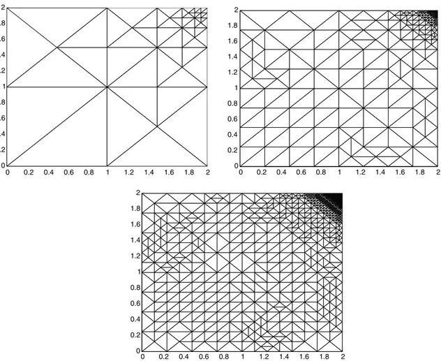
Fig. 3. Adapted intermediate meshes with 577, 4079, and 16 738 degrees of freedom, respectively, for Example 1.
We first consider the linear version of the boundary value problem (1.1) on the square X:¼ ð0;2Þ ð0;2Þ. We take the kinematic viscosity function w1, and choose the data f and g so that the exact solution of (1.1) is, respectively, for Examples 1 and 2,
u1ðxÞ:¼ ðð4:1x1x2Þ 1=3
;ð4:1x1x2Þ 1=3
Þt; p1ðxÞ:¼x1þx2;
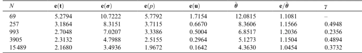
Table 5
Individual errors, error estimate~h, effectivity index, and rate of convergence for the uniform refinement (Example 3)
N eðtÞ eðrÞ eðpÞ eðuÞ ~h e=~h c
69 5.2794 10.7222 5.7792 1.7154 12.0815 1.1081 – 257 3.1864 8.3151 3.7115 0.6670 8.3606 1.1566 0.4948 993 2.7048 7.0207 3.3386 0.5004 6.8517 1.2036 0.2356 3905 2.3132 4.7988 2.5155 0.2964 5.1273 1.1504 0.4894 15 489 2.1680 3.4936 1.9672 0.1642 4.3630 1.0454 0.3732
0 0.2 0.4 0.6 0.8 1 1.2 1.4 1.6 1.8 2 0
0.2 0.4 0.6 0.8 1 1.2 1.4 1.6 1.8 2
0 0.2 0.4 0.6 0.8 1 1.2 1.4 1.6 1.8 2 0
0.2 0.4 0.6 0.8 1 1.2 1.4 1.6 1.8 2
0 0.2 0.4 0.6 0.8 1 1.2 1.4 1.6 1.8 2 0
0.2 0.4 0.6 0.8 1 1.2 1.4 1.6 1.8 2
and
u2ðxÞ:¼ ðð4:01x1x2Þ 3=4
;ð4:01x1x2Þ 3=4
Þt; p2ðxÞ:¼x1þx2;
for all x:¼ ðx1;x2Þ 2X. We notice that u1 and u2 are divergence free in X and singular in an exterior neighborhood of the pointð2;2Þ.
In Tables 1–4, we give the errors for each unknown (excepteðnÞ, which converges very rapidly to zero), the error estimate~h, the effectivity indexe=~h, and the experimental rate of convergencecfor the uniform and adaptive refinements. The individual and global errors are computed on each triangle using a 7 points Gaussian quadrature rule (see [9]). We observe here that the effectivity indexes are bounded above and below, which confirms the reliability of the a posteriori estimate ~h (cf. Theorem 2.1), and provides
Table 6
Individual errors, error estimate~h, effectivity index, and rate of convergence for the adaptive refinement (Example 3)
N eðtÞ eðrÞ eðpÞ eðuÞ ~h e=~h c
69 5.2794 10.7222 5.7792 1.7154 12.0815 1.1081 – 202 3.2431 9.6118 4.3531 0.8386 8.1037 1.3661 0.3538 326 1.8141 5.8557 1.1372 0.3873 6.0926 1.0253 2.3911 528 1.1815 3.7349 0.2741 0.2353 4.1806 0.9410 1.9183 730 0.8565 2.3970 0.2993 0.2173 2.8618 0.8988 2.6230 1667 0.5601 1.5001 0.2795 0.1477 1.8178 0.8979 1.1017 3590 0.3975 1.0074 0.1671 0.1134 1.2672 0.8694 1.0246 9034 0.2528 0.6283 0.0978 0.0717 0.8054 0.8543 1.0200 15 492 0.1893 0.4895 0.0690 0.0531 0.6230 0.8539 0.9542 36 185 0.1265 0.3115 0.0468 0.0355 0.4049 0.8427 1.0473
Table 7
Individual errors, error estimate~h, effectivity index, and rate of convergence for the uniform refinement (Example 4)
N eðtÞ eðrÞ eðpÞ eðuÞ ~h e=~h c
69 5.5291 20.7907 6.9546 1.6773 20.9411 1.0827 – 257 3.7377 14.9927 3.5568 0.7641 15.4037 1.0305 0.5421 993 2.9702 11.6530 3.2730 0.5219 11.8187 1.0554 0.3568 3905 2.4196 7.9531 2.4870 0.2999 8.3101 1.0448 0.5292 15 489 2.2007 5.1378 1.9601 0.1646 5.8258 1.0171 0.5547
Table 8
Individual errors, error estimate~h, effectivity index, and rate of convergence for the adaptive refinement (Example 4)
N eðtÞ eðrÞ eðpÞ eðuÞ ~h e=~h c
69 5.5291 20.7907 6.9546 1.6773 20.9411 1.0827 – 111 5.3733 17.1622 6.6382 1.5643 17.6647 1.0890 0.6916 317 4.3304 14.4414 6.3571 1.2294 13.3123 1.2328 0.3026 878 3.0736 10.7921 4.8276 0.7634 9.6218 1.2721 0.5758 1109 1.2380 7.3492 0.6084 0.1824 7.6423 0.9787 4.2166 1537 0.9658 5.1429 0.4443 0.1657 5.4367 0.9664 2.1642 2979 0.6404 3.1625 0.3380 0.1353 3.3701 0.9635 1.4544 4411 0.5447 2.5478 0.3043 0.1328 2.7265 0.9633 1.0810 10 140 0.3987 1.6597 0.2001 0.1017 1.8212 0.9453 1.0148 16 879 0.2809 1.3344 0.1452 0.0658 1.4366 0.9557 0.8881 42 271 0.1941 0.8190 0.0909 0.0478 0.9025 0.9396 1.0498
numerical evidences for it being efficient. Then, Figs. 1 and 2 showeversus the degrees of freedomN for Examples 1 and 2. In each case the total erroreof the adaptive algorithm decreases much faster than that of the uniform one. In particular, the slow convergence observed in the uniform refinement of Example 2 is considerably improved by the corresponding adaptive strategy. These facts are also emphasized by the experimental rates of convergence provided in the tables, which show that the adaptive method recovers the order of convergence guaranteed by Theorem 3.2 in [5], that is OðhÞ. Next, Figs. 3 and 4 display some intermediate meshes obtained with the refinement procedure. We remark, as expected, that the algorithm is able to recognize the neighborhood of the singularpointð2;2Þin both examples.
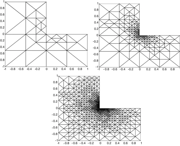
We now consider the full nonlinear boundary value problem (1.1) on the L-shaped domain X:¼ ð1;1Þ2 ð0;1Þ2. We take the kinematic viscosity functionwas given by the Carreau law withj0¼j1¼ 1=2 andb¼3=2 (see Section 1 in [5]), that iswðtÞ:¼1
2þ
1 2ð1þt
2Þ1=4
, and choose the dataf andgso that the exact solution of (1.1) is, respectively, for Examples 3 and 4,
u3ðxÞ:¼ ðx1
h
0:1Þ2þ ðx20:1Þ2
i1=2
ðx20:1;0:1x1Þt; p3ðxÞ:¼ð 2 x1x2Þ1=2;
Fig. 5. Total errorefor uniform and adaptive refinements (Example 3).
and
u4ðxÞ:¼ ðx1
h
0:1Þ2þ ðx20:1Þ 2i1=2
ðx20:1;0:1x1Þ t
; p4ðxÞ:¼1=ðx11:1Þ;
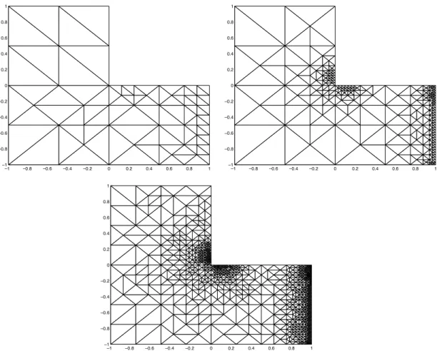
for all x:¼ ðx1;x2Þ 2X. We note that u3 and u4 are divergence free in X and singular in an exterior neighborhood ofð0;0Þ. In addition, the singularity of p4runs along the line x1¼1:1.
Similarly as for the linear case, we present in Tables 5–8 the errors for the main unknowns, the error estimate~h, the effectivity indexe=~h, and the experimental rate of convergencec. The discrete scheme (1.6) is solved by NewtonÕs method with an initial guess given by the solution of the linear problem (w1), and a tolerance of 103 for the relative error. The number of iterations needed in each mesh is 3 (for both examples). Next, Figs. 5 and 6 showeversus the degrees of freedomN, and Figs. 7 and 8 provide some intermediate meshes obtained with the refinement method.
The remarks and conclusions here are the same of the linear examples. In particular, the effectivity indexes confirm the reliability of~hand constitute experimental evidences of an eventual efficiency. Further, the adaptive procedure leads again to the quasi-optimal linear rate of convergence, and it is able to identify the singularities of each problem. This means, as observed in Figs. 7 and 8, that the adapted meshes are
1 0.8 0.6 0.4 0.2 0 0.2 0.4 0.6 0.8 1 1
0.8 0.6 0.4 0.2 0 0.2 0.4 0.6 0.8 1
1 0.8 0.6 0.4 0.2 0 0.2 0.4 0.6 0.8 1 1
0.8 0.6 0.4 0.2 0 0.2 0.4 0.6 0.8 1
1 0.8 0.6 0.4 0.2 0 0.2 0.4 0.6 0.8 1 1
0.8 0.6 0.4 0.2 0 0.2 0.4 0.6 0.8 1
-- - - -
-- - - -
-- - - -
-Fig. 7. Adapted intermediate meshes with 528, 3590, and 15 492 degrees of freedom, respectively, for Example 3.
highly refined around the point ð0;0Þ for Examples 3 and 4, and also around the segment x1¼1:0 for Example 4.
Summarizing, the results presented in this section provide enough support for the adaptive algorithm being much more efficient than a uniform discretization procedure when solving the mixed finite element scheme (1.6).
Acknowledgements
This research was partially supported by CONICYT-Chile through the FONDAP Program in Applied Mathematics, and by the Direccion de Investigaci on of the Universidad de Concepcion through the Ad-
vanced Research Groups Program.
References
[1] R.E. Bank, A. Weiser, Some a posteriori error estimators for elliptic partial differential equations, Math. Computat. 44 (1985) 283–301.
–1 –0.8 –0.6 –0.4 –0. 2 0 0.2 0.4 0.6 0.8 1 –1
–0.8 –0.6 –0.4 –0.2 0 0.2 0.4 0.6 0.8 1
–1 –0.8 –0.6 –0.4 –0.2 0 0.2 0.4 0.6 0.8 1 –1
–0.8 –0.6 –0.4 –0.2 0 0.2 0.4 0.6 0.8 1
–1 –0.8 –0.6 –0.4 –0.2 0 0.2 0.4 0.6 0.8 1 –1
–0.8 –0.6 –0.4 –0.2 0 0.2 0.4 0.6 0.8 1
[2] M.A. Barrientos, G.N. Gatica, E.P. Stephan, A mixed finite element method for nonlinear elasticity: two-fold saddle point approach and a-posteriori error estimate, Numerische Mathematik 91 (2) (2002) 197–222.
[3] U. Brink, E. Stein, A posteriori error estimation in large-strain elasticity using equilibrated local Neumann problems, Comput. Methods Appl. Mech. Engrg. 161 (1998) 77–101.
[4] U. Brink, E.P. Stephan, Adaptive coupling of boundary elements and mixed finite elements for incompressible elasticity, Num. Methods Partial Diff. Equat. 17 (2001) 79–92.
[5] G.N. Gatica, M. Gonzalez, S. Meddahi, A low-order mixed finite element method for a class of quasi-Newtonian Stokes flows. Part I: a-priori error analysis, Comput. Methods Appl. Mech. Engrg. 193 (6–8) (2004), to be published.
[6] G.N. Gatica, N. Heuer, E.P. Stephan, An implicit-explicit residual error estimator for the coupling of dual-mixed finite elements and boundary elements in elastostatics, Math. Methods Appl. Sci. 24 (2001) 179–191.
[7] G.N. Gatica, E.P. Stephan, A mixed-FEM formulation for nonlinear incompressible elasticity in the plane, Num. Methods Partial Diff. Equat. 18 (1) (2002) 105–128.
[8] J.-L. Lions, E. Magenes, Problemes aux Limites non Homogenes et Applications I, Dunod, Paris, 1968. [9] A. Stroud, Approximate Calculation of Multiple Integrals, Prentice-Hall, Englewood Cliffs, 1971.
[10] R. Verf€urth, A Review of A Posteriori Error Estimation and Adaptive Mesh-Refinement Techniques, Wiley-Teubner, Chichester, 1996.