Título60 GHz Millimeter Wave Propagation Inside Bus: Measurement, Modeling, Simulation, and Performance Analysis

Received May 30, 2019, accepted June 18, 2019, date of publication June 24, 2019, date of current version August 6, 2019. Digital Object Identifier 10.1109/ACCESS.2019.2924729

60-GHz Millimeter-Wave Propagation Inside Bus:

Measurement, Modeling, Simulation, and

Performance Analysis

ANIRUDDHA CHANDRA 1, (Senior Member, IEEE), ANIQ UR RAHMAN1, (Student Member, IEEE), USHASI GHOSH1_{, (Student Member, IEEE), JOSÉ A. GARCÍA-NAYA} 2_{, (Member, IEEE),}

ALEŠ PROKEŠ 3, JIRI BLUMENSTEIN 3, (Member, IEEE), AND

CHRISTOPH F. MECKLENBRÄUKER 4, (Senior Member, IEEE)

1_{Department of Electronics and Communication Engineering, National Institute of Technology, Durgapur 713209, India} 2_{CITIC Research Center, Universidade da Coruña, 15071 A Coruña, Spain}

3_{Department of Radio Electronics, Brno University of Technology, 61200 Brno, Czech Republic}

4_{Christian Doppler Laboratory, Institute of Telecommunications, Vienna University of Technology, 1030 Vienna, Austria}

Corresponding author: Aleš Prokeš ([email protected])

This work was supported in part by the Czech Science Foundation through the Project Mobile Channel Analysis and Modelling in Millimeter Wave Band, under Grant 17-27068S, and in part by the National Sustainability Program through Interdisciplinary Research of Wireless Technologies under Grant LO1401. The work of A. Chandra was supported in part by the Core Research Grant (CRG), Science and Engineering Research Board, Department of Science and Technology, Government of India, under Grant CRG/2018/000175, and in part by the Research Initiation Grant (RIG), NIT Durgapur, under Grant 996/2017. The work of J. A. García-Naya was supported in part by the Xunta de Galicia under Grant ED431C 2016-045, Grant ED341D R2016/012, and Grant ED431G/01, in part by the Agencia Estatal de Investigación of Spain under Grant TEC2015-69648-REDC and Grant TEC2016-75067-C4-1-R, and in part by the ERDF funds of the EU (AEI/FEDER, UE).

ABSTRACT Millimeter-wave (mmWave) transmission over the unlicensed 60-GHz spectrum is a potential solution to realize high-speed internet access, even inside mass transit vehicles. The solution involves communication between users and a mmWave-band on-board unit that aggregates/disseminates data streams from/to commuters and maintains the connection with the nearest terrestrial network infrastructure node. In this paper, we provide a measurement-based channel model for the 60-GHz mmWave propagation inside a typical inter-city bus. The model characterizes power delay profile (PDP) of the wireless intra-vehicular channel, and it is derived from about 1000 data sets measured within the bus. The proposed analytical model is further translated into a simple simulation algorithm that generates in-vehicle channel PDPs. Different goodness-of-fit tests confirm that the simulated PDPs are in good agreement with the measured data. Finally, a tapped-delay-line (TDL) channel model is formulated from the proposed PDP model, and the TDL model is used to study the bit error rate (BER) performance of the mmWave link inside bus under varying data rates and link lengths.

INDEX TERMS Intra-vehicular communication, 60 GHz channel sounding, power delay profile, tapped delay line, bit error rate.

I. INTRODUCTION

Remaining connected while on-the-move is the mantra of the next generation commuters [1]. Over the last two decades, there had been a steady increase in long distance commuting as a result of urbanization of employment opportunities [2]. According to the European Union (EU) labor force survey conducted in 2015, 8% of the EU workforce commuted to

The associate editor coordinating the review of this manuscript and approving it for publication was Ke Guan.

work in a different region, and 1% commuted cross-border. The average commute time per day is about 1.1 hours [3], with around 10% extreme commuters spending more than 2 hours per day [4]. Driving personal cars for commuting is a unproductive task and leads to unnecessary stress. By letting someone else to do the driving, connected commuters can utilize the unpaid time for working, gathering information, or enjoying multimedia streaming [5].

For a daily commuter, public transport vehicles (e.g., buses, trains, and ferries) are cost-effective and

FIGURE 1. Network access during commute.

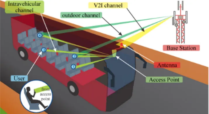
environmentally friendly alternatives, providing easy access to major urban joints and alleviating the user from parking worries. On top of that, policymakers are working hard to achieve car-free cities [6], [7] through subsidies and aware-ness campaigns. In spite of these, the shift in the commuting mode is sluggish [8]–[10] and the transportation sector is in desperate need of a game changer. A large section of stakeholders believe that equipping public vehicles with on-board gigabit wireless networks can accelerate the shift considerably. The idea is illustrated in Fig.1, where the access network forms a two-hop system: base stations (BSs) or road side units (RSUs) serve the vehicular access point (AP) over vehicle-to-infrastructure (V2I) mobile channels, and the vehicular AP connects to the passengers inside over static intravehicular channels.1 The network architecture helps in avoiding the penetration loss caused by metallic bodies and signaling overhead due to group handovers [1] experienced in direct outdoor channels. There are many other potential appli-cations of intravehicular wireless signaling beyond user con-nectivity, which include counting the number of passengers in a public vehicle [11] or establishing a small-scale social networking platform between co-passengers [12]. However, wireless communication infrastructures inside public vehi-cles should be able to provide such on-demand real-time high-data-rate diverse services.

Millimetre wave (mmWave) is a promising new technology [13] which is able to provide an enormous band-width to support the aforementioned diverse services in cur-rent fifth generation (5G) [14] and beyond 5G [15] networks. There had been already several initiatives to implement mmWave in intelligent transportation systems [16], [17]. In the 60 GHz unlicensed band, mmWave networks can provide up to 100 Gbit/s [18] in short-range limited-mobility scenarios, i.e., inside offices and buildings [19]–[21], or in specialized environments such as inside vehicles.

1_{The outdoor channel referred in Fig.1is basically an outdoor-to-indoor}

channel penetrating the vehicle and is used by a commuter to directly connect with a BS or RSU when there is no provision of connecting to an in-vehicle AP. Further, the AP needs to be equipped with two antennas, one outside the vehicle, which connects to the nearest BS/ RSU and has a wired connection to the AP fitted inside the vehicle, and another inside the vehicle attached to the AP, which connects to the user devices.

In general, mmWave propagation is significantly distinct when compared to narrowband sub-6 GHz propagation in several respects [22]: sparse multipath, high path-loss, direc-tional transmission, lesser penetration, diffuse scattering, etc. In a closed space environment such as interior of a vehicle, the effect of some of these characteristics is magnified. Thus, experimental study of intravehicle mmWave propagation channel is of fundamental interest.

The 60 GHz mmWave propagation was earlier inves-tigated for links between cars [23]–[25], for links inside cars [26]–[29], and for links inside aircrafts [30], [31]. Recent works also compare the 60 GHz mmWave transmis-sion to the traditional ultra-wideband (UWB) transmistransmis-sion in the 3-11 GHz band [32]–[34]. However, mmWave channel models inside public transport vehicles such as buses have rarely been studied in depth. Previous works include nar-rowband measurements at 2.4 GHz [35], at 5 GHz [36], [37], and UWB measurements in the range of 2.3-11 GHz [38]. The only exceptions are [39] or authors’ own works such as [40] and [41], in which some initial measurement data and preliminary channel modeling is presented for 60 GHz mmWave signal propagation inside a bus.

The electronic communications committee (ECC) recom-mendation on using 57-64 GHz band in 2009 [42] paved the way for 60 GHz mmWave-based pan-European cross-border experiments on connected and automated driving [43]. Stan-dardization and regulation of such EU cooperative intelligent transport systems (C-ITSs) [44] is driven by car-2-car com-munication consortium (C2C-CC), European telecommuni-cations standards institute (ETSI) and European committee for standardization (CEN). In this regard, the present work is the outcome of the collaboration between research groups in three different countries, namely Czech Republic, Austria, and Spain, in which we focus on intravehicular communi-cations. The main contributions of this paper are detailed below.

• We provide measurement data for 60 GHz frequency-domain channel sounding inside a bus. Around a thou-sand data points have been recorded during the field trials. Instead of using a vector network analyzer (VNA) (which has range limitations due to the cable costs), we employed a signal analyzer, enabling us to cover the whole bus length.

FIGURE 2. Measurement setup [left]. The bus from outside [right-top] and inside [right-bottom].

• Power delay profiles (PDPs) are obtained from the frequency-domain sounding data by means of the complex-valued inverse fast Fourier transform (IFFT). General PDP trends are identified, which helped to perform an analytical characterization and subsequently led to a simple PDP simulation algorithm which requires only the receiver-transmitter distance d as an input. Additionally, the performance of the algorithm has been evaluated and validated with several goodness-of-fit (GoF) tests.

• Discrete-time PDPs are derived from the continuous-time PDPs, hence the channel can be modeled as a tapped-delay-line (TDL) filter for link-level simulations. The entire simulation code along with the recorded data set is made available through IEEE Code Ocean plat-form (DOI: 10.24433/CO.1876676.v1). The TDL model is used to study the bit error rate (BER) performance of the mmWave link inside the bus with varying data rates and link lengths.

The rest of the paper is organized as follows. In Section II, we discuss the experimental setup employed for the channel measurements. The post processing method using the Hilbert transform is presented in Section III. In Section IV, we discuss our analytical PDP model and introduce the PDP simulation algorithm. Section V presents of the TDL model and the results of the BER simulations. Finally, Section VI concludes the paper.

II. FIELD EXPERIMENTS

Field experiments were performed at Brno University of Technology campus in Czech Republic. The vehicle used is a 50-seater long-distance inter-city coach (model: Mercedes Benz Tourismo BlueTec4), parked in front of a covered garage. There were no other cars on the parking lot during

measurements and the immediate surroundings have no buildings or concrete structures. The bus has a dimension of 12 m (length) by 2.5 m (width) by 3.3 m (height). Inside, the floor-to-ceiling distance is 2 m, the overhead luggage rack is at 1.7 m height and each seat is 1.25 m high. The half-rows are 0.95 m wide on each side with an aisle space of 0.5 m in-between, and the distance between successive seat rows is 0.75 m. The exterior and interior of the bus is shown in Fig.2.

FIGURE 3. Placement of the antennas inside the bus [left], photographs of the antenna assemblies [middle], and simulated radiation patterns of the antennas both in the E-plane and in the H-plane [right].

connected to the VNA, facing large cable losses and thus limiting the Tx-Rx distance.

A bandwidth (BW) of 10 GHz was covered, ranging from 55GHz to 65 GHz and 60 GHz being the center frequency. 1001 measurement points were recorded in each sweep. A complete sweep requires 4 minutes. The CTF amplitude, |H(f)|, is recorded for each frequency point (fi;fi+1−fi = 10 MHz). The output of the signal generator is sent, by means of a cable, to the PA, which is powered by the DC power supply and exhibits a gain to compensate for the cable losses and also to boost the signal to be fed to the open waveguide type Tx antenna (OWGA). At the receiver end, the signal is captured by a substrate-integrated-waveguide slot antenna (SIW SA) and is sent to the signal analyzer. Given that the signal analyzer can only work up to 50 GHz, an external mixer down-converts the signal to an intermediate frequency (IF) of 404.4 MHz, mitigating also the high cable losses at mmWave frequencies.

The position of the Tx and the Rx antennas inside the bus is shown in Fig. 3. Since our goal is to evaluate the performance of the 60 GHz downlink channel, the Rx antenna is attached to a drop-down seat tray, imitating the typical position of a handheld personal wireless device. To cover the entire space inside the bus, the Rx antenna was placed at 15 different seats during the course of the measurements. On the other hand, the position of the Tx antenna is placed near the ceiling and the bust front window to emulate a rooftop access point. The close-up of the antenna fixtures is also shown in Fig. 3. The absorbers are used to limit reflections from metal parts of the fixtures. There are a number of WR 15 type waveguides used between the PA

and the Tx antenna to point the antenna towards the desired direction.

As shown in Fig.3, the radiation pattern of the Rx antenna is omni-directional (mobile user), whereas the Tx antenna (access point) is a directional waveguide, whose main beam is directed towards the seats to maximize directivity.

III. POST PROCESSING

Measurement setups based on VNAs are favored to carry out frequency-domain static wireless channel measurements/ sounding due to their robustness and high dynamic range. In spite of a static channel environment inside a bus, a VNA-based setup could not be employed for the channel measure-ments because the measurement distance would then have been restricted by the length of the coaxial cables. Contrarily, a signal analyzer cannot measure directly the phase of the captured signals, but the phase can be retrieved from the amplitude only measurement data to produce the complex-valued CTF. The complex-complex-valued IFFT can then be applied to procure the channel response in the time domain.

those papers can be demonstrated in the following manner. The complex-valued CTF in the frequency-domain can be written in polar form as

H(jω)= |H(jω)|exp(jarg[H(jω)]), (1)

and taking logarithms on both sides we have ˜

H(jω)=log_e{|H(jω)|} +jarg[H(jω)], (2)

where log_e{H(jω)} =log_e{|H(jω)|} +jarg[H(jω)]. Defining ˜

h(n) = F−1_[H(j˜ _{ω)] as the Fourier inverse ofH}˜_{(jω), then} the phase information can be obtained from the amplitude response [45] as follows

arg[H(jω)]=H[log_e{|H(jω)|}], (3)

whereH[·] denotes the Hilbert transform assuming thath(n)˜ is causal, i.e.,h(n)˜ =0; n<0.

A. PROPOSED METHOD

In this subsection, we present our HT based approach to recover the phase information. The CTF need not be a mini-mum phase function in this case. However, it must be a causal function, a significantly weaker condition inflicted on the channel response.

The objective is to project the amplitude data into the real-valued component of the regenerated CTF employing the HT. Consequently, the phase delay is first derived as a function of the frequency. The phase difference (1φ), path difference (1x), wavelength (λ), speed of light (c) and frequency (f) are related as1φ =2π1x/λandc=λf. During our mea-surements, we recorded the Tx-Rx distance (d) for each pair of Tx-Rx combinations, which we use as the path difference. Combining the above mentioned equations, the phase delay function is then defined as:

φd(f)=(2π d f)/c. (4)

The Tx-Rx propagation delay is compensated by the phase delay function,φd(f), hence the phase information appears right from the line-of-sight (LoS)/ strongest arrival path instant. The real-valued part is obtained as the cosine com-ponent of the CTF magnitude:

Re{ ˜H(f)})= |H(f)| cos{φd(f)}. (5)

This real-valued part is then fed as the argument of the hilbert operator:

ˆ

H(f)=H[Re{ ˜H(f)}], (6)

that generates the complex-valued CTF,H(fˆ ). After applying the IFFT [48] on it, the corresponding PDP realization is obtained.

B. VALIDATION AND COMPARISON

To prove the validity/ accuracy of our method, we take advan-tage of the previous measurement campaign [29] in which 60 GHz intra-vehicular channel sounding was carried out in a sedan car employing a VNA. The phase data is first

FIGURE 4. CTF amplitude measured and generated [car data].

FIGURE 5. CTF phase measured and generated [car data].

removed from the recorded measurements and then we try to regenerate the complex-valued CTF,H(fˆ ), following the method proposed in the previous subsection.

Figs.4and5show the retrieved amplitude and phase plots, respectively, corresponding to a specific Rx-Tx position. This procedure is performed for all the data sets corresponding to the various Rx-Tx settings. The results have exhibited excellent agreement between both the estimated amplitude and phase plots and the true measurement data.

Next, IFFT is applied to the regenerated complex-valued CTFs which are then utilized to produce the PDPs. This is then compared with the PDPs produced directly by applying the IFFT on the VNA recorded data. Fig.6presents the PDP plots for four exemplary Tx-Rx settings. The generated PDPs closely resemble the corresponding measured PDP trails.

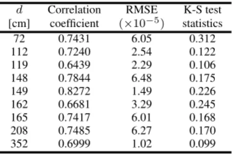
Table1summarizes the goodness-of-fit (GoF) results that gauge the similarity between the generated and the measured values of the PDP. We have considered three GoF metrics, correlation coefficient, root mean square error (RMSE) and Kolmogorov-Smirnov (K-S) test statistic. The correlation coefficient (ρˆ) has been modeled according to [49]:

ˆ

ρ=

1 N

PN

n=1|P(n)||Pg(n)|

q 1 N

PN

n=1|P(n)|2 1N

PN

n=1|Pg(n)|2

, (7)

FIGURE 6. PDPs measured and generated [car data].

TABLE 1. GoF between measured and generated PDPs.

has been evaluated as [50]

RMSE=

r

1 N

XN

n=1(|P(n)| − |Pg(n)|)

2, ₍₈₎

and the two-sample K-S test has been evaluated according to [51]

K =max[F(|P(n)|)−_F(|_Pg(n)|)], (9)

whereK denotes the statistic test of the K-S test and F is the cumulative distribution function (CDF). The high values of the correlation coefficients demonstrate the existence of a strong association between the generated and the measured data. Low values of the RMSE between the two datasets and the two-sample K-S test statistic calculated with a 5% significance level corroborates the claim.

The efficacy of the proposed method is further proven as the time dispersion parameters are also estimated, i.e, the mean delay time (τ¯) and the root mean square (RMS) delay spread (τrms). These are the first moment and the second central moment of the PDP, respectively, and they are defined as [52]

¯

τ =

Pτmax τ=0τP(τ) Pτmax

τ=0P(τ)

, and (10)

TABLE 2.Measured and generated time-delay parameters.

τrms=

s Pτmax

τ=0(τ− ¯τ)2P(τ) Pτmax

τ=0P(τ)

, (11)

whereP(τ)=E{|h(τ)|2}is the received power at time-delay

τ, i.e., the PDP; E{·} is the expectation operator and τ is a discrete-time vector defined at the nonzero values of the CIR (h(τ)), varying between 0 and a maximum time-delay (τmax). Table2affirms our proposed approach by comparing the time dispersion parameters,τ¯ andτrms, of the measured and generated data sets.

Finally, the supremacy of our proposed approach is estab-lished as we analyze the same data with the approach pro-posed in [46], in which a blind Hilbert approach has been considered which is available in any commercial mathemat-ical software package such as MATLAB. It does not exploit the Tx-Rx distance information available in the measurement data set. Fig.7shows the generated PDP and CTF from the method in [46], proving that applying basic HT can yield inaccurate results.

IV. PDP MODELLING AND SIMULATION

The propagation environment inside a bus is different from the conventional indoor scenarios, and often this can be attributed to the general construction of the interior of the bus. It was shown in [40] that although a higher value of path loss (PL) is expected at mmWave frequencies, it is possible to reach even the back seats of the bus with a single AP antenna mounted on the top of the driver seat at the front side of the bus. The reason behind this was the low value of PL coefficient, which was close to the free-space case, and this fact may be attributed to the metallic body of the bus which behaved as a waveguide and facilitated the wave propagation. The right side of a long distance commuter bus also have a different construction compared to the left side, with doors, staircases, place for toilet/ WC and a TV screen. This caused an additional PL of 2-3 dB. However, the effect of upholstery or curtains was not very significant.

FIGURE 7. Generated PDP and CTF using the method proposed in [46]. The same car data is used to obtain the figures. Comparison of Fig. 7b with Fig.4and Fig. 7a with Fig.6shows that basic HT can give inaccurate results while the proposed modified HT gives accurate results.

FIGURE 8. General PDP trends inside the bus.

1) When viewed in log scale, the PDPs decay in a nonlin-ear manner.

2) Again, in the log scale, the gross decay slope across the PDPs are quite close for identicald values.

3) There exists a power law relationship between the peak amplitude, say,A(d), andd, across the PDPs. In the log-log scale, this is reflected as a linear decrease of the peak amplitude with distance.

4) The PDP values oscillate between a lower bound and an upper bound. The interval between the two boundaries does not change significantly with time delay.

A. ANALYTICAL PDP MODEL

From these observations, we may assume a PDP function of the form

fd(τ)=A(d) exp[B(d)τ], (12)

where, as defined earlier,A(d) is the peak amplitude while B(d) denotes the decay rate, and both are functions of d. A visual inspection inspires us to set power-law relation for

FIGURE 9. log(A(d)) versus log(d) regression plot.

both the functions, i.e.A(d)=αdmandB(τ)=βdn, which describesfd(τ) as

fd(τ)=αdmexp(βdnτ). (13)

The empirical values of log(A(d)) with log(d) are plotted across several experiments in Fig.9. Consequently, the values m= −1.3891 andα= −5.434×10−2are obtained from the line of best-fit.

From (13) we can write log_efd(τ)/(αdm)

/τ =βdn. (14)

From the regression plot in Fig.9, it is possible to obtain the values forαandm. Next, with the help of (14), we can find the maximum likelihood values ofβandnin a similar manner for all experiments (the corresponding fittings are omitted for brevity). After analyzing and calibrating the values ofβ and nacross all the measured experimental data sets, we set them ton= −0.4 andβ = −1×10−12.

Next, we define an adjustable boundary function, b(τ), to account for the variations between the upper and the lower bounds,

b(τ)=

1+ρlog

τ τscale

+1

fd(τ), (15)

This boundary function helps us define the upper limit (bU) and the lower limit (bL) of the PDP as

bU(τ)=(1−B/100+ε)b(τ), (16)

and

bL(τ)=(1+ε)b(τ), (17)

whereBis the range of the PDP values expressed in dBm units andεlowers the PDP curve by 100εdBm. The following set of values,ε=0.005,B=10, was found to be optimum.

The simulated PDP,Ps(τ), for every time delayτ, can be finally obtained by generating a uniformly distributed random number,

Ps(τ)=U(bL(τ),bU(τ)), (18)

where, U(·,·) returns a uniform random number ranging between its arguments.

B. SIMULATION OF PDP

The method of generating PDP, which is discussed in Section IV-A in detail, is summed up in this subsection in the form of a pseudocode (see Algorithm1). Our simulation algorithm takes Tx-Rx distance (d) as input and returns simu-lated channel PDP (Ps(τ)) as output. The algorithm produces a continuous-time PDP starting from zero to a maximum time delayτmaxwith a sampling rateτres = 1/BW. Considering the dimensions of the bus, the parameterτmaxis set to 50 ns.

Algorithm 1Channel PDP Simulation

Input: d [Tx-Rx distance]

Assignments: [Parameters]

α← −5.434×10−2;β← −1×10−12;m← −1.3891; n← −0.4;B←10;ρ←0.09;ε←0.005;

τ ←0;τscale ←10;τres←10−10;τmax←50×10−9 1: whileτ ≤τ_maxdo

2: fd(τ):=αdmexp(βdnτ) 3: b(τ):=1+ρlog

τ τscale +1

fd(τ) 4: bU(τ):=(1−B/100+ε)b(τ) 5: bL(τ):=(1+ε)b(τ)

6: Ps(τ):=U(bL(τ),bU(τ)) 7: τ :=τ +τ_res

8: end while

Output: Ps(τ) [Simulated channel PDP]

A sample simulated PDP is shown in Fig.10along with the PDP obtained from the measurement data. The generated and measured PDPs compare pretty well with a strong correlation, the coefficient being greater than 0.7.

C. VALIDATION OF THE SIMULATION METHOD

To assess the performance of the simulation model, the same set of GoF tests are employed as done in Section III-B, with replacingPg(n) withPs(n), wherePs(n) denote the data points for simulated PDPs. The values correlation coefficient, RMS error and K-S test are enlisted for 9 cases in Table3.

FIGURE 10. Simulated PDP [d=972 cm,ρˆ=0.7230].

TABLE 3.GoF between measured and simulated PDPs.

FIGURE 11. CDFs of both measured and simulated PDPs.

The comparison is performed for all the measured test points, and PDPs calculated from the measured CTFs are compared to the corresponding PDPs simulated with the measured d value. In order to validate the proposed intravehicle channel model simulation, we have visualized the CDFs from the two-sample K-S test shown in Fig.11for a typical measurement scenario with a Tx-Rx separation of 5.16 m.

Finally, in Fig.12we show a comparison of the time dis-persion parameters for the measured and the generated data sets using a comparative bar graph, showing how closely the simulated channel time dispersion parameters resemble the measured channel parameters across all the 9 experimental data sets.

V. BER PERFORMANCE ANALYSIS

FIGURE 12. Measured and simulated time-delay parameters.

terms of the bit error rate (BER), which requires to discretize the PDP and derive an equivalent TDL model.

A. TDL MODEL

In a multipath fading wireless channel, if there exists a small number of distinctive multipath components (MPCs) or if the multipath components can be grouped into clusters where the path delays between clusters can be resolved but the MPC delays within a cluster are non-resolvable, then the channel can be modeled in the time-domain as a tapped-delay-line (TDL) filter. In the TDL model, delays between taps dif-ferentiate one scatterer group from the other and each tap represents the contribution of an individual scatterer group. The impulse response for the channel in this case can be conveniently expressed in the form [53]

h(t, τ)= N−1 X

i=0

Giγi(t)δ(τ−τi), (19)

whereN is the total number of taps, andGi,γi(t) andτi are the gain, small-scale fading and delay of the (i+1)th tap, respectively.

For our model we considered a uniform delay ofτi+1− τi = 5 ns between taps and for aτmax = 50 ns,2the TDL model consisted ofN =10 taps. The first tap is normalized (G0 = 0 dB,γ0 = 1), denoting the LoS/ strongest path, whereas the remaining tap gains are derived by sampling the simulated PDP and the small-scale fading coefficients follow-ing a Rayleigh process, γi ∼ CN(0,1), where CN(µ, σ2) denotes circularly symmetric complex-valued Gaussian ran-dom variable with meanµand varianceσ2. Fig. 13shows a typical channel realization obtained following our TDL model.

In Table 4, we enlist the tap gains obtained from the simulated PDPs for all the taps and for four different Tx-Rx separations. The distance values are chosen to represent dif-ferent sections of the bus; a d value of 1.66 m (2.35 m) denotes the second (third) row from the front, the distance is 5.76 m to the seat near the middle door, and in the back seat d goes up to 9.72 m. As one can notice, the tap gains decay

2_{PDP record of 50 ns ensured that propagation paths having a path length}

of up to 15 m with multiple bounces inside the bus are taken into account. The differential delay of 5 ns symbolizes a data rate of 200 Mbit/s which can be changed by resampling of the PDP to obtain a TDL model having a different delay gap.

FIGURE 13. Sample TDL realization [d=3.70 m].

TABLE 4.Tap gain for differentdvalues.

FIGURE 14. Block diagram for BER simulation.

sharply at the front rows, whereas at the back seat, the tap gain remains constant for the last four to five taps. The slow decrease of the tap gain indicates that the effect of multipath will be much more prominent at the back seats.

B. SIMULATION OF BER

FIGURE 15. BER curves for different data rates.

During the simulation, a bit-stream ofBN =106data bits3 were transmitted through the channel after modulation. The modulated signal is defined as

x(t)= BN X

k=0 ˆ

x(k)δ(t−kτp), (20)

whereτpis the sampling period of the input which, assuming a simple binary phase shift keying (BPSK) modulation, i.e.

ˆ

x(k)∈ {+1,−1}, rendersR=1/τpto be the transmitted bit rate andEb=E{ ˆx2(k)}τpto be the energy transmitted per bit. The modulated signal is fed as the input to the multipath fading channel. The tap coefficients for various distances are taken from Table 4. The received signal is, y(t) = x(t)∗ h(t)+n(t), where∗denotes the convolution operator andn(t) is additive Gaussian white noise (AWGN) with double-sided power spectral densityN0/2. The outputy(t) is truncated from t = 0 tot = BNτp and demodulated to recover the input signal. The demodulated bit-stream,y(t), is deduced asˆ

ˆ

y(k)=sign{y(t−kτp)}, (21)

and is compared to x(k). The number of mismatches areˆ divided byBN to compute the BER. During the simulations, BER is determined as a function of the signal-to-noise ratio (SNR),Eb/N0.

Fig.15shows the BER variation with different data rates for a fixeddvalue of 1.66 m. BER curves are shown for three different data rates, 50 Mbit/s, 100 Mbit/s and 200 Mbit/s. These data rates are comparable to data rates available with wired cable modem or 4G cellular LTE networks. Fig. 15

shows that the SNR requirement may go up by 10 dB when the required data rate doubles. For lower bit rates, the effect of inter-symbol interference is reduced, as the information bits are spaced out. The AWGN BER curve is also shown as a reference.

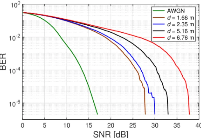
Next, we plot the BER curves for varying Tx-Rx dis-tances in Fig. 16 keeping the bit rate fixed at 100 Mbit/s. As the distance increases, the multipath environment degrades the signal. In our case, the access point is placed in front, so the back seat passenger experiences an additional

3_{Each time an averaging over 10}3_{runs were performed to test BER up to}

the range 10−7.

FIGURE 16. BER curves for different Tx-Rx distances.

SNR penalty of about only 10 dB compared to the front row passengers. This observation nullifies the myth that mmWave cannot propagate over larger distances in confined environ-ments. The BER curves indicate that if a proper link margin is maintained, it is possible to use 60 GHz hardware to provide broadband access with desired reliability.

VI. CONCLUSION

The article presents measurement-based modeling and per-formance evaluation of 60 GHz mmWave wireless link inside a bus. Comprehensive measurements are conducted to study the PDP behavior which led to the development of an ana-lytical framework followed by an algorithmic flowchart to simulate PDPs. Simulated PDP values are used to derive a TDL equivalent link model which forms the basis for link performance evaluation. It is observed that the distance of the user from the access point and the specified data rate has a large impact on the BER performance of the intrave-hicular mmWave link. Although the modeling and analysis is carried out for a bus, the characterization is applicable for other public transport vehicles (e.g. subway coaches, trams and trolleybuses) which have similar internal structures and comparable dimensions.

ACKNOWLEDGMENT

For the research, the infrastructure of the SIX Center was used.

REFERENCES

[1] J. Kim, H. Chung, G. Noh, S. W. Choi, I. Kim, and Y. Han, ‘‘Overview of moving network system for 5G vehicular communications,’’ inProc. IEEE EuCAP, Apr. 2019, pp. 1–5.

[2] M. Andersson, N. Lavesson, and T. Niedomysl, ‘‘Rural to urban long-distance commuting in Sweden: Trends, characteristics and pathways,’’ J. Rural Stud., vol. 59, pp. 67–77, Apr. 2018.

[3] A. Künn-Nelen, ‘‘Does commuting affect health?’’Health Econ., vol. 25, no. 8, pp. 984–1004, Aug. 2016.

[4] S. Vincent-Geslin and E. Ravalet, ‘‘Determinants of extreme commuting. Evidence from Brussels, Geneva and Lyon,’’J. Transp. Geography, vol. 54, pp. 240–247, Jun. 2016.

[6] M. Nieuwenhuijsen, J. Bastiaanssen, S. Sersli, E. O. D. Waygood, and H. Khreis, ‘‘Implementing car-free cities: Rationale, requirements, barriers and facilitators,’’ inProc. Integrating Hum. Health Urban Transp. Plan-ning, Jul. 2018, pp. 199–219.

[7] M. J. Nieuwenhuijsen and H. Khreis, ‘‘Car free cities: Pathway to healthy urban living,’’Environ. Int., vol. 94, pp. 251–262, Sep. 2016.

[8] C. Calastri, S. Borghesi, and G. Fagiolo, ‘‘How do people choose their commuting mode? An evolutionary approach to travel choices,’’Economia Politica, vol. 13, pp. 1–26, Feb. 2018.

[9] A. Lieberoth, N. H. Jensen, and T. Bredahl, ‘‘Selective psychological effects of nudging, gamification and rational information in converting commuters from cars to buses: A controlled field experiment,’’Transp. Res. Part F, Traffic Psychol. Behav., vol. 55, pp. 246–261, May 2018. [10] N. Hoang-Tung, A. Kojima, and H. Kubota, ‘‘Impacts of travellers’ social

awareness on the intention of bus usage,’’IATSS Res., vol. 39, no. 2, pp. 130–137, Mar. 2016.

[11] T. A. Myrvoll, J. E. Håkegård, T. Matsui, and F. Septier, ‘‘Counting public transport passenger using WiFi signatures of mobile devices,’’ inProc. IEEE 20th Int. Conf. Intell. Transp. Syst. (ITSC), Oct. 2017, pp. 1–6. [12] S. Maaroufi and S. Pierre, ‘‘Vehicular social systems: An overview and a

performance case study,’’ inProc. ACM DIVANet, Montreal, QC, Canada, Sep. 2014, pp. 17–24.

[13] M. Xiao, S. Mumtaz, Y. Huang, L. Dai, Y. Li, M. Matthaiou, G. K. Karagiannidis, E. Björnson, K. Yang, I. Chih-Lin, and A. Ghosh, ‘‘Millimeter wave communications for future mobile networks,’’IEEE J. Sel. Areas Commun., vol. 35, no. 9, pp. 1909–1935, Sep. 2017. [14] A. Al-Dulaimi, X. Wang, and I. Chih-Lin,5G Networks:

Fundamen-tal Requirements, Enabling Technologies, and Operations Management. Hoboken, NJ, USA: Wiley, 2018.

[15] K. David and H. Berndt, ‘‘6G vision and requirements: Is there any need for beyond 5G?’’IEEE Veh. Technol. Mag., vol. 13, no. 3, pp. 72–80, Sep. 2018.

[16] L. Kong, M. K. Khan, F. Wu, G. Chen, and P. Zeng, ‘‘Millimeter-wave wireless communications for IoT-cloud supported autonomous vehicles: Overview, design, and challenges,’’IEEE Commun. Mag., vol. 55, no. 1, pp. 62–68, Jan. 2017.

[17] I. Mavromatis, A. Tassi, R. J. Piechocki, and A. Nix, ‘‘Efficient millimeter-wave infrastructure placement for city-scale ITS,’’ Mar. 2019, arXiv:1903.01372. [Online]. Available: https://arxiv.org/abs/1903.01372 [18] Y. Ghasempour, C. R. C. M. D. Silva, C. Cordeiro, and E. W. Knightly,

‘‘IEEE 802.11 ay: Next-generation 60 GHz communication for 100 Gb/s Wi-Fi,’’IEEE Commun. Mag., vol. 55, no. 12, pp. 186–192, Dec. 2017. [19] A. Bamba, F. Mani, and R. D’Errico, ‘‘Millimeter-wave indoor channel

characteristics in V and E bands,’’IEEE Trans. Antennas Propag., vol. 66, no. 10, pp. 5409–5424, Oct. 2018.

[20] A. W. Mbugua, K. Saito, F. Zhang, and W. Fan, ‘‘Characterization of human body shadowing in measured millimeter-wave indoor channels,’’ inProc. IEEE 29th Annu. Int. Symp. Pers., Indoor Mobile Radio Commun. (PIMRC), Bologna, Italy, Sep. 2018, pp. 1–5.

[21] S. Li, Y. Liu, L. Lin, D. Sun, S. Yang, and X. Sun, ‘‘Simulation and modeling of millimeter-wave channel at 60 GHz in indoor environment for 5G wireless communication system,’’ inProc. IEEE Int. Conf. Comput. Electromagn. (ICCEM), Mar. 2018, pp. 1–3.

[22] A. F. Molisch, A. Karttunen, R. Wang, C. U. Bas, S. S. Korea, S. S. Korea, and J. Zhang, ‘‘Millimeter-wave channels in urban environments,’’ inProc. 10th Eur. Conf. Antennas Propag. (EuCAP), Apr. 2016, pp. 1–5. [23] W. Schafer and E. Lutz, ‘‘Propagation characteristics of short-range

radio links at 60 GHz for mobile intervehicle communication,’’ inProc. SBT/IEEE Int. Symp. Telecommun., Rio de Janeiro, Brazil, Sep. 1990, pp. 212–216.

[24] D. L. Didascalou, F. Kuchen, and W. Wiesbeck, ‘‘An investigation of millimeter wave propagation mechanisms for mobile intervehicle com-munications and outdoor MBS,’’ inProc. 48th IEEE Veh. Technol. Conf. Pathway Global Wireless Revolution, May 1998, pp. 1800–1804. [25] A. Kato, K. Sato, M. Fujise, and S. Kawakami, ‘‘Propagation

characteris-tics of 60-GHz millimeter waves for ITS inter-vehicle communications,’’ IEICE Trans. Commun., vol. 84, no. 9, pp. 2530–2539, Sep. 2001. [26] H. Sawada, T. Tomatsu, G. Ozaki, H. Nakase, S. Kato, K. Sato, and

H. Harada, ‘‘A sixty GHz intra-car multi-media communications system,’’ inProc. IEEE 69th Veh. Technol. Conf., Apr. 2009, pp. 1–5.

[27] K. Fujita, H. Sawada, and S. Kato, ‘‘Intra-car communications system using radio hose,’’ inProc. IEEE Asia–Pacific Microw. Conf., Dec. 2010, pp. 57–60.

[28] R. Nakamura and A. Kajiwara, ‘‘Empirical study on 60GHz in-vehicle radio channel,’’ in Proc. IEEE Radio Wireless Symp., Jan. 2012, pp. 327–330.

[29] A. Chandra, P. Kukolev, T. Mikulášek, and A. Prokeš, ‘‘Frequency-domain in-vehicle channel modelling in mmW band,’’ inProc. IEEE 1st Int. Forum Res. Technol. Soc. Ind. Leveraging Better Tomorrow (RTSI), Sep. 2015, pp. 106–110.

[30] M. Peter, W. Keusgen, A. Kortke, and M. Schirrmacher, ‘‘Measurement and analysis of the 60 GHz in-vehicular broadband radio channel,’’ inProc. IEEE 66th Veh. Technol. Conf., Sep. 2007, pp. 834–838.

[31] R. Felbecker, W. Keusgen, and M. Peter, ‘‘Ray-tracing simulations of the 60 GHz incabin radio channel,’’ inProc. URSI GASS, Aug. 2008, pp. 1–4. [32] M. Schack, M. Jacob, and T. Kiirner, ‘‘Comparison of in-car UWB and 60 GHz channel measurements,’’ inProc. IEEE 4th Eur. Conf. Antennas Propag., Apr. 2010, pp. 1–5.

[33] J. Blumenstein, A. Prokes, A. Chandra, T. Mikulasek, R. Marsalek, T. Zemen, and C. Mecklenbräuker, ‘‘In-vehicle channel measurement, characterization and spatial consistency comparison of 3-11 GHz and 55-65 GHz frequency bands,’’IEEE Trans. Veh. Technol., vol. 66, no. 5, pp. 3526–3537, May 2017.

[34] A. Prokes, T. Mikulasek, J. Blumenstein, C. F. Mecklenbrauker, and T. Zemen, ‘‘Intra-vehicle ranging in ultra-wide and millimeter wave bands,’’ inProc. IEEE Asia–Pacific Conf. Wireless Mobile (APWiMob), Aug. 2015, pp. 246–250.

[35] L. Azpilicueta, P. L. Iturri, E. Aguirre, J. J. Astrain, J. Villadangos, C. Zubiri, and F. Falcone, ‘‘Characterization of wireless channel impact on wireless sensor network performance in public transportation buses,’’ IEEE Trans. Intell. Transp. Syst., vol. 16, no. 6, pp. 3280–3293, Dec. 2015. [36] H. Suzuki, Z. Chen, and I. B. Collings, ‘‘Analysis of practical MIMO-OFDM performance inside a bus based on measured channels at 5.24 GHz,’’ inProc. IEEE 2nd Eur. Conf. Antennas Propag. EuCAP, Nov. 2007, pp. 1–8.

[37] D. W. Matolak and A. Chandrasekaran, ‘‘5 GHz intra-vehicle channel characterization,’’ inProc. IEEE Veh. Technol. Conf., Sep. 2012, pp. 1–5. [38] B. Li, C. Zhao, H. Zhang, X. Sun, and Z. Zhou, ‘‘Characterization

on clustered propagations of UWB sensors in vehicle cabin: Mea-surement, modeling and evaluation,’’IEEE Sensors J., vol. 13, no. 4, pp. 1288–1300, Apr. 2013.

[39] V. Semkin, A. Ponomarenko-Timofeev, A. Karttunen, O. Galinina, S. Andreev, and Y. Koucheryavy, ‘‘Path loss characterization for intra-vehicle wearable deployments at 60 GHz,’’ Jan. 2019,arXiv:1902.01949. [Online]. Available: https://arxiv.org/abs/1902.01949

[40] A. Chandra, T. Mikulasek, J. Blumenstein, and A. Prokes, ‘‘60 GHz mmW channel measurements inside a bus,’’ inProc. IEEE 8th IFIP Int. Conf. Technol., Mobility Secur., Larnaca, Cyprus, Nov. 2016, pp. 1–5. [41] A. U. Rahman, U. Ghosh, A. Chandra, and A. Prokes, ‘‘Channel modelling

for 60GHz mmWave communication inside bus,’’ inProc. IEEE Veh. Netw. Conf. (VNC), Taipei, Taiwan, Dec. 2018, pp. 1–6.

[42] I. Karls and M. Mueck, ‘‘V2X requirements, standards, and regulations,’’ inNetworking Vehicles to Everything: Evolving Automotive Solutions. Berlin, Germany: De Gruyter, 2018, ch. 3, pp. 59–88.

[43] E. Uhlemann, ‘‘Continued dispute on preferred vehicle-to-vehicle tech-nologies,’’IEEE Veh. Technol. Mag., vol. 12, no. 3, pp. 17–20, Sep. 2017. [44] K. Sjoberg, P. Andres, T. Buburuzan, and A. Brakemeier, ‘‘Cooperative intelligent transport systems in Europe: Current deployment status and outlook,’’IEEE Veh. Technol. Mag., vol. 12, no. 2, pp. 89–97, Jun. 2017. [45] B. P. Donaldson, M. Fattouche, and R. W. Donaldson, ‘‘Characterization

of in-building UHF wireless radio communication channels using spectral energy measurements,’’IEEE Trans. Antennas Propag., vol. 44, no. 1, pp. 80–86, Jan. 1996.

[46] A. Prokes, T. Mikulasek, J. Blumenstein, and J. Vychodil, ‘‘Usability of Hilbert transform for complex channel transfer function calculation in 60 GHz band,’’ inProc. PIERS, Nov. 2017, pp. 2945–2951.

[47] M. Kyrö, S. Ranvier, V. M. Kolmonen, K. Haneda, and P. Vainikainen, ‘‘Long range wideband channel measurements at 81-86 GHz frequency range,’’ inProc. IEEE 4th Eur. Conf. Antennas Propag. EuCAP, Barcelona, Spain, Apr. 2010, pp. 1–5.

[48] T. Domínguez-Bolaño, J. Rodríguez-Piñeiro, J. A. García-Naya, and L. Castedo, ‘‘Experimental characterization of LTE wireless links in high-speed trains,’’Wireless Commun. Mobile Comput., vol. 2017, pp. 1–20, Sep. 2017.

[50] R. J. Hyndman and A. B. Koehler, ‘‘Another look at measures of forecast accuracy,’’Int. J. Forecasting, vol. 22, no. 4, pp. 679–688, Oct. 2006. [51] F. J. Massey, Jr., ‘‘The Kolmogorov-Smirnov test for goodness of fit,’’

J. Amer. Statist. Assoc., vol. 46, no. 3, pp. 68–78, 1951.

[52] A. J. Goldsmith,Wireless Communications. Cambridge, U.K.: Univ. Press, 2005.

[53] T. Blazek, M. Ashury, C. F. MecklenbrÃďuker, D. Smely, and G. Ghiaasi, ‘‘Vehicular channel models: A system level performance analysis of tapped delay line models,’’ inProc. IEEE 15th Int. Conf. ITS Telecommun. (ITST), Warsaw, Poland, May 2017, pp. 1–8.

ANIRUDDHA CHANDRA (M’08–SM’16)

received the B.E., M.E., and Ph.D. degrees from Jadavpur University, Kolkata, India, in 2003, 2005, and 2011, respectively. He joined the Electron-ics and Communication Engineering Department, National Institute of Technology, Durgapur, India, in 2005, where he is currently an Associate Pro-fessor. In 2011, he was a Visiting Lecturer with the Asian Institute of Technology, Bangkok. From 2014 to 2016, he was a Marie Curie Fellow with the Brno University of Technology, Czech Republic. He has published about 80 research papers in refereed journals and peer-reviewed conferences. His research interest includes physical layer issues in wireless communication. He was a co-recipient of the Best Short Paper Award at the IEEE VNC 2014, Paderborn, Germany, and delivered a keynote lecture at the IEEE MNCApps 2012, Bengaluru, India.

ANIQ UR RAHMAN(S’18) is currently pursuing the B.Tech. degree with the Department of Elec-tronics and Communication Engineering, National Institute of Technology, Durgapur (NITD), India, where he also serves as the Chair of the IEEE Student Branch. He was a Summer Intern with the European Organization for Nuclear Research (CERN), Switzerland, in 2018. He is also an Avid Programmer and an Open Source Enthusiast and was accepted in the Google Summer of Code Pro-gram, in 2017, where he was a Software Developer Intern with Robocomp, Universidad de Extremadura, Spain, in 2017. His research interests include wireless communication, signal processing, and the Internet of Things.

USHASI GHOSH (S’18) is currently pursuing the degree with the Department of Electronics and Communication Engineering, National Insti-tute of Technology, Durgapur, India. She was a Summer Research Intern with the IIT Kanpur, Kanpur, India, in 2018. Prior to that, she was also a Research Intern with the IIT Hyderabad, India. Her research interest includes the broad area of wireless communications.

JOSÉ A. GARCÍA-NAYA(S’07–M’10) received the M.Sc. and Ph.D. degrees in computer engi-neering from the University of A Coruña (UDC), A Coruña, Spain, in 2005 and 2010, respectively, where he has been with the Group of Electron-ics Technology and Communications, since 2005, and is currently an Associate Professor. He is the coauthor of more than 90 peer-reviewed papers in journals and conferences. His research interests include the experimental evaluation of wireless systems in realistic scenarios (indoors, outdoors, high mobility, and railway transportation), signal processing for wireless communications, wireless sensor networks, specially devoted to indoor positioning systems, and time-modulated antenna arrays applied to wireless communication systems. He is also a member of the research team of more than 40 research projects funded by public organizations and private companies.

ALEŠ PROKEŠreceived the M.Sc., Ph.D., and Habilitation degrees from the Brno University of Technology (BUT), in 1988, 1999, and 2006, respectively, where he has been with the Faculty of Electrical Engineering and Communication, since 1990, and is currently a Professor. Since 2013, he has been the Head of the Research Cen-ter of Sensor, Information and Communication Systems, and Radio-Frequency Systems Group. He has coauthored 30 journal publications and more than 40 conference papers. His research interests include measurement and modeling of channels for V2X communication, optimization, and design of optical receivers and transmitters for free-space optics (FSO) systems, influence of atmospheric effects on optical signal propagation, evaluation of FSO availability and reliability, higher order non-uniform sampling and signal reconstruction, and software-defined radio.

JIRI BLUMENSTEIN(M’17) received the Ph.D. degree from the Brno University of Technology, in 2013. In 2011, he was a Researcher with the Institute of Telecommunications, TU Wien. He has cooperated with several companies, includ-ing Racom, Volkswagen, and ON Semiconductor, in the areas of applied research of wireless systems and fundamental research funded by the Czech Science Foundation. He is currently a Researcher with the Department of Radio Electronics, Brno University of Technology. His research interests include signal processing, physical layer of communication systems, channel characterization and mod-eling, and wireless system design.

CHRISTOPH F. MECKLENBRÄUKER (S’88–