DIFFERENCE LIMENS FOR MEASURES OF APPARENT SOURCE WIDTH

(1)

DIFFERENCE LIMENS FOR MEASURES OF APPARENT SOURCE WIDTH

PACS REFERENCE: 43.55.Br

Blau, Matthias

TU Dresden

Institut f ¨ur Akustik und Sprachkommunikation D–01062 Dresden

Tel.: +49 351 463 33041 Fax: +49 351 458 37510 Email: Matthias.Blau@epost.de

ABSTRACT

Apparent source width (ASW) is thought of being one important component of spatial impression in concert halls. The validity of known objective measures that correlate with ASW, namelyLF_E4

andIACC_E3_{, has recently been questioned as measurements of these quantities in concert halls}

revealed significant fluctuations over small spatial intervals. In a first step towards assessing the perceptual relevance of these fluctuations, listening tests aimed at finding a threshold difference below which changes in perceived ASW are no longer relevant for concert halls were carried out. The results of these tests are discussed together with implications for further research.

1 INTRODUCTION

Apparent source width (ASW) is thought of being one important component of spatial impres-sion in concert halls. As spatial impresimpres-sion is considered a major acoustical attribute of halls, it should be taken into account in the design of new, or in the modification of existing, halls. In order to aid the design process, objective measures (i.e. quantities that can be measured in existing halls or models of halls) have been developed.

In the case of ASW, these objective measures include the strength factor at low frequencies, as well as the early parts of the lateral fraction, the interaural cross-correlation coefficient (all of which are defined in the appendix to ISO 3382 [1]) and that of TRAUTMANN’s criterion RL _[2].

All of these measures, with perhaps the exception of the strength factor, are subject of ongoing discussions [1, 3, 2, 4].

One major point of criticism is that these measures can fluctuate considerably over small spatial intervals (one and the same seat), both in concert halls [5] and in virtual sound fields [6]. Whereas most people argue that one will usually not perceive differences in ASW over one and the same seat, it was recently shown that one can create pairs of plausible virtual sound fields whose differences in ASW are judged differently when the subjects lean towards the left or the right side of the seat [6].

To aid future investigations into this field, it would be helpful to have difference limens for the known objective measures, i.e. differences below which no change in ASW is perceived. On the other hand, investigations into difference limens must take into account that, even in a listening experiment with well controlled parameters, there may be fluctuations of the objective measures depending on the actual position of the subject’s head. This latter fact appears to be completely ignored in the work on difference limens for objective measures published so far.

(2)

[image:2.595.105.489.72.332.2]

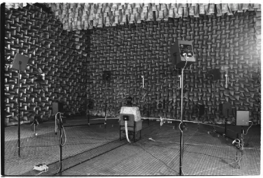
Figure 1: Listening test: set-up.

2 LISTENING TESTS: METHOD

Listening tests were carried out in the anechoic room of Institut f ¨ur Akustik und Sprachkom-munikation (room free volume: 1000m3_{, low-frequency limit: 60Hz). The test set-up is shown in} fig. 1. Subjects were seated in the center of a circular louspeaker array (radius 3m) which served to produce virtual sound fields based on anechoic music (a continuous repetition of bars 560/561 of the first movement of the Symphony No. 4 in E-flat by BRUCKNER, taken from the CD “Ane-choic Orchestral Recordings” by DENON). All experiments were carried out in the dark in order to exclude visual cues. The virtual sound fields consisted of the direct sound (originating from the loudspeaker in front of the subject) plus eight reflections with varying level and delay (delivered by loudspeakers at±30◦, ±45◦, ±60◦, ±85◦, respectively). The sound fields were generated randomly by imposing the following conditions:

1. the larger the angle of incidence, the larger the delay,

2. reflections with symmetric angles of incidence were required to be at least 3ms apart,

3. reflection levels were chosen from a modifiedχ2-distribution with given mean and maximum values which in turn were varied but always decreased with increasing delays,

4. the total energy of the reflection was adjusted such that it was within 0.5dB of that of the direct sound.

(3)

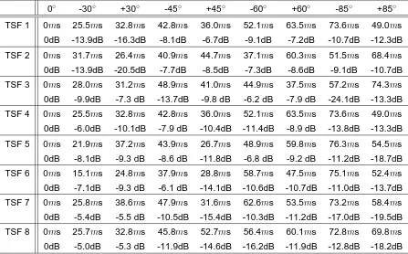
0◦ _-30◦ ₊₃₀◦ _-45◦ ₊₄₅◦ _-60◦ ₊₆₀◦ _-85◦ ₊₈₅◦

TSF 1 0ms 25.5ms 32.8ms 42.8ms 36.0ms 52.1ms 63.5ms 73.6ms 49.0ms

0dB -13.9dB -16.3dB -8.1dB -6.7dB -9.1dB -7.2dB -10.7dB -12.3dB

0dB -13.9dB -20.5dB -7.7dB -8.5dB -7.3dB -8.6dB -9.1dB -10.7dB

0dB -9.9dB -7.3 dB -13.7dB -9.8 dB -6.2 dB -7.9 dB -24.1dB -13.3dB

0dB -6.0dB -10.1dB -7.9 dB -10.4dB -11.4dB -8.9 dB -13.8dB -13.3dB

0dB -8.1dB -9.3 dB -8.6 dB -11.8dB -6.8 dB -9.2 dB -11.2dB -18.7dB

TSF 6 0ms 15.1ms 24.8ms 37.9ms 28.8ms 58.7ms 47.5ms 75.1ms 52.4ms 0dB -7.1dB -9.3 dB -6.1 dB -14.1dB -10.6dB -10.7dB -11.0dB -13.7dB

0dB -5.4dB -5.5 dB -10.5dB -15.4dB -10.3dB -11.2dB -17.0dB -19.5dB

[image:3.595.86.533.72.350.2]

0dB -5.0dB -5.3 dB -11.9dB -14.6dB -16.2dB -11.9dB -12.8dB -18.2dB

Table 1: Listening test: Parameters of the eight test sound fields. Given are delays and levels for reflections arriving under the indicated angles of incidence.

the absolute value of the scale values was decreased by 0.5 in order to rejoin positive and neg-ative scales after the enforced split in the first step. As complete sets of pair-comparisons were tested, the consistency of the judgements could be verified: All subjects achieved a coefficient of consistency of at least 0.8. Each session lasted about 30min.

All signal processing and the test control was provided by a Personal Computer running jMax 2.5.1 (IRCAM), equipped with a 16-channel audio interface (RME Digi9632 + Creamware A16). Objective measures were calculated on the basis of measured binaural impulse responses (arti-ficial head: Neumann KU-80). As the calculation ofRL_E _{involves the determination of the sine}

of incidence angles of 2ms long sections of the first 80ms of the binaural impulse response, one can derive a modified lateral energy fractionLFC0

Efrom it,

LFC0

E= PW

i=1Eisinϕi ED+PW_i=1Ei

. (1)

In this equation, Ei andϕi are the energy and the angle of incidence of theith section of the binaural impulse response andED is the energy of the direct sound. Because of the directional characteristics of the artificial head, values ofLFC0

E are different from (higher than) what would be measured with the classical combination of figure-of-eight and omnidirectional microphones. However, both are highly correlated, withLFC0_E4_{being about 2.4 times}LF_E4_{for the sound fields}

studied here.

Although the position of the subject’s head was predetermined to a certain degree by the seat, it was not explicitely enforced to be the same for all subjects. Therefore, the impulse responses were measured on a grid of 8×8cm (every 2cm) in the head plane.

In addition to the octave-band averaged values of IACC_E_, RL_E _and LFC0

E (i.e. IACCE3,

RL_E6_andLFC0

E4, withE3: 500Hz. . . 2kHz,E4: 125Hz. . . 1kHz,E6: 125Hz. . . 4kHz), broadband versions based on low-pass (at 6kHz) filtered impulse responses were considered as well. These measures are referred to asIACC_Ebb_,RL_Ebb_andLFC0_Ebb_{, respectively. Measured values ranged}

(4)

R²=0.8

dIACC_E3

−0.05 0

0.05

Subjective Scale of ASW

−4 −2 0 2 4

R²=0.69

dIACC_Ebb

−0.05 0

0.05

[image:4.595.117.480.73.245.2]

Subjective Scale of ASW

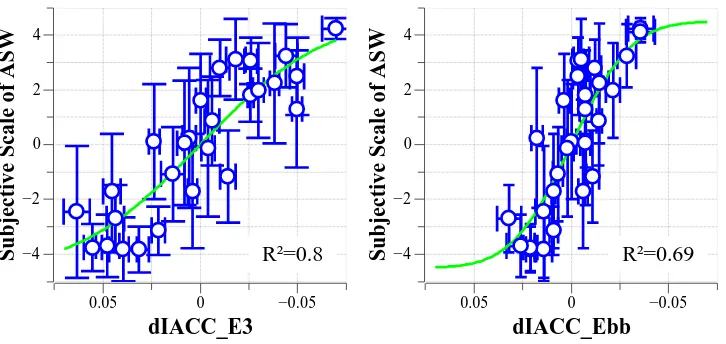
−4 −2 0 2 4

Figure 2: Listening test: subjective judgements of ASW versus differences inIACC_E. Circles represent means, vertical error bars 95% confidence intervals for the mean of the judgements, horizontal error bars 95% confidence intervals for the mean of the difference inIACC_E. The solid curve is the model for the means, according to eq. 2. Left:IACC_E3. Right:IACCEbb.

3 LISTENING TESTS: RESULTS

In fig. 2, subjective scale values for individual test pairs are plotted versus the differences inIACC_E_{. For both versions of the}IACC_E_{, the correlation between judgements and objective}

measures is fairly good. However, for the broad-band version the change in the judgements is much larger for a given difference inIACC_E_{. Conversely, the values (and the differences) of the} IACCEbbare within much smaller limits than those of theIACCE3.

An inspection of the confidence intervals for the means of both the subjective judgements and the difference inIACC_E_{suggests that the influence of spatial variations in}IACC_E _{over the area}

where the subjects’ heads were, is not very important (compared to that of the fluctuations in the subjective judgements).

The appearance of the relation between subjective scale values and differences in the objec-tive measure suggests that a linear model with saturation for large absolute differences inIACC_E

could be used. The model adopted here is a modified error integral,

mean judgement=

( _√9 π

R|dIACCE|

0 e

(ξ/σ)2

dξ if dIACC_E≤0

−√9

π

R|dIACCE|

0 e

(ξ/σ)2

dξ if dIACC_E_>0 . (2)

This model was iteratively (inσ) fitted to the means of both the subjective judgements and the differences inIACC_E_.

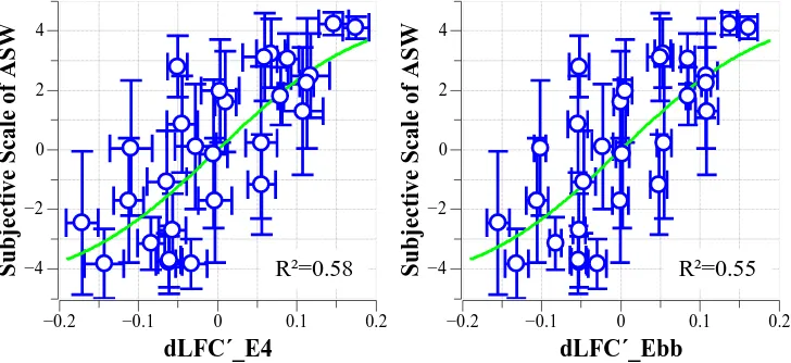
Similar analyses were carried out forRL_E _and LFC0_E_{, see figs. 3 and 4. In comparison to} IACC_E_{, the correlation between judgements and objective measures is not as good, and}

differ-ences between octave-band averaged and broad-band versions of the measures are negligeable.

4 DISCUSSION

In the preceding section, results of listening tests were presented in the form of subjective scale values of differences in ASW, as a function of differences in the objective measures. To derive difference limens from these relations, H ¨OHNEand SCHROTH[7] proposed to consider the value of the objective measure at which the value of the model function is±2.5. This means that the average (experienced) listener will perceive a small difference in ASW, under ideal listening conditions and in a pair-comparison scenario. It is the author’s belief that this proposal is a sensible criterion for the difference limen, if different seats in a hall are to be compared.

Following this proposal, the difference limen for theIACC_E3_{would turn out to be 0.038, and}

(5)

R²=0.61

dRL_E6 in dB

−2 0 2

Subjective Scale of ASW

−4 −2 0 2 4

R²=0.61

dRL_Ebb in dB

−2 0 2

[image:5.595.117.477.74.246.2]

Subjective Scale of ASW

−4 −2 0 2 4

Figure 3: Listening test: subjective judgements of ASW versus differences inRL_E. Circles represent means, vertical error bars 95% confidence intervals for the mean of the judgements, horizontal error bars 95% confidence intervals for the mean of the difference inRL_E. The solid curve is the model for the means, according to eq. 2 (where dIACC_E must be substituted by−dRLE). Left:RLE6. Right:RLEbb.

R²=0.58

dLFC´_E4

−0.2 −0.1 0 0.1 0.2

Subjective Scale of ASW

−4 −2 0 2 4

R²=0.55

dLFC´_Ebb

−0.2 −0.1 0 0.1 0.2

Subjective Scale of ASW

−4 −2 0 2 4

Figure 4: Listening test: subjective judgements of ASW versus differences inLFC0

E. Circles represent

means, vertical error bars 95% confidence intervals for the mean of the judgements, horizontal error bars 95% confidence intervals for the mean of the difference inLFC0

E. The solid curve is the model for the means,

according to eq. 2 (where dIACC_E must be substituted by−dLFC0E). Left:LFC0E4. Right:LFC0Ebb.

If the difference limen forLF_E4_{is estimated from that of}LFC0_E4_{(using the factor 2.4 mentioned}

in section 2) or from that of theIACC_E3_{(using a logarithmic model of data by B}ERANEK[8]), a value of 0.045. . . 0.07 is obtained.

The difference limen for the IACC_E3 _{found here is somewhat lower than the values found}

recently by OKANO[4] (0.05. . . 0.07) or that found by COXet al. for theIACC_E4_{[9] (0.075). The}

most likely reason for this (small) discrepancy is that in those investigations, only the level of one or more reflections was altered whereas in the work presented here, completely different sound fields were compared. A relatively low difference limen forIACC_E _{is however consistent with}

results from investigations on the perception of spatial fluctuations of theIACC _[6].

As was seen in section 3, theIACC_E_{gave the best correlation with the subjective judgements}

in the tests presented here. However, previous investigations [2, 10] have shown that this is not consistently the case. Instead, the IACC_E _{sometimes produced predictions which largely}

underestimated the subjective judgements. Future work is needed to clarify this issue.

[image:5.595.117.481.334.501.2]

(6)

mea-sures.

5 CONCLUSION

In this paper, investigations aiming at finding difference limens for measures of apparent source width (ASW) were presented. As opposed to work published so far, spatial fluctuations over the area of the subjects’ head of the objective measure in question were controlled, and a pair comparison technique in which both level and delays of all reflections were altered was used. Using a criterion proposed by H ¨OHNEand SCHROTH, the difference limen for theIACC_E3_was

found to be 0.038, for values of theIACC_E3_{between 0.3 and 0.42. For the corresponding value}

ofRL_E6_{between -3.8dB and +0.7dB, the difference limen was found to be 1.8dB. The difference}

limen forLF_E4_{can be estimated from the difference limen of the}IACC_E3_{and from that of}LFC0 E4. For a value of theLF_E4_{between 0.18 and 0.26, this estimate is 0.045. . . 0.07.}

Future work is needed to cover other ranges of the objective measures and to clarify the origin of some outliers that theIACC_E_{produced in previous listening tests.}

References

[1] ISO 3382:1997, Acoustics - Measurement of the reverberation time of rooms with reference to other acoustical parameters.

[2] A. Then and M. Blau. Vergleich ausgew ¨ahlter objektiver raumakustischer Parameter hin-sichtlich ihrer Korrelation mit dem subjektiven Kriterium “Scheinbare Breite der Quelle” bei Musikdarbietungen. In Fortschritte der Akustik - DAGA 2001, Oldenburg, 2001. DEGA e.V.

[3] T. Okano, L.L. Beranek, and T. Hidaka. Relations among interaural cross-correlation coef-ficient (IACCE), lateral fraction (LFE), and apparent source width (ASW) in concert halls. JASA, 104:255–265, 1998.

[4] T. Okano. Judgements of noticeable differences in sound fields of concert halls caused by intensity variations in early reflections. JASA, 111:217–229, 2002.

[5] D. de Vries, Hulsebos. E.M., and J. Baan. Spatial fluctuations in measures for spaciousness. Journal of the Acoustical Society of America, 110:947–954, 2001.

[6] M. Blau. Untersuchungen zur Wahrnehmbarkeit ¨ortlicher Schwankungen von R ¨aumlichkeitsparametern bei Musikdarbietungen. In Fortschritte der Akustik - DAGA 2002, Oldenburg, 2002. DEGA e.V.

[7] R. H öhne and G. Schroth. Zur Wahrnehmbarkeit von Deutlichkeits- und Durchsichtigkeitsun-terschieden in Zuh örers älen. Acustica, 81:309–319, 1995.

[8] L. L. Beranek. Concert and opera halls: How they sound. Acoustical Society of America, 1996.

[9] T. Cox, W.J. Davies, and Y.W. Lam. The sensitivity of listeners to early sound field changes in auditoria. Acustica, 79:27–41, 1993.