Contents lists available atScienceDirect
Physica A
journal homepage:www.elsevier.com/locate/physa
Pattern synchrony in electrical signals related to earthquake activity
R. Hernández-Pérez
a,d,∗, L. Guzmán-Vargas
b, A. Ramírez-Rojas
c, F. Angulo-Brown
daSatélites Mexicanos, S.A. de C.V., Centro de Control Satelital Iztapalapa. Av. de las Telecomunicaciones S/N CONTEL Edif. SGA-II. México, D.F. 09310, Mexico bUnidad Profesional Interdisciplinaria en Ingeniería y Tecnologías Avanzadas, Instituto Politécnico Nacional, Av. IPN No. 2580, Col. Ticomán, México D.F. 07340,
Mexico
cDepartamento de Ciencias Básicas, Universidad Autónoma Metropolitana, Av. San Pablo 180, Col. Reynosa, México D.F., 02200, Mexico
dDepartamento de Física, Escuela Superior de Física y Matemáticas, Instituto Politécnico Nacional, Edif. 9 U.P. Zacatenco, México D.F. 07738, Mexico
a r t i c l e i n f o
Article history:
Received 19 August 2009
Received in revised form 13 November 2009
Available online 4 December 2009
Keywords:
Seismicity Time series analysis Complexity Statistical methods Pattern synchrony
a b s t r a c t
We apply the cross sample entropy method to geoelectrical time series collected from inde-pendent channels (North–South and East–West directions) monitored at two sites located in Mexico, to assess the presence of pattern synchrony between the signals, particularly in the proximity of earthquakes. To our best knowledge, this method has not been applied yet for the study of electrical signals related to earthquake activity. Moreover, we introduce the multiscale pattern synchrony analysis by extending the multiscale entropy technique to calculate the cross-entropy between two signals, which represents a novel approach to the study of pattern synchrony. The results obtained suggest that in the vicinity of an earth-quake the geoelectrical signals exhibit pattern synchrony that persists for long sequences and through multiple scales, in addition to the presence of correlations in each channel.
©2009 Elsevier B.V. All rights reserved.
1. Introduction
There have been many studies on developing a robust meaning ofcomplexity, noticeably in physiological signals where complexity has been associated to healthy systems [1–5], and particularly in electrical signals related to earthquake activity [6–24]. With respect to the electroseismic signals, the study of electromagnetic phenomena that were possibly associated with earthquakes (EQs) was developed by Varotsos and Alexopoulos in 1984, through the introduction of the VAN method, which is based on the premise that large EQs are preceded by observable anomalous changes in the geoelectrical potential called seismic electric signals (SES) [25,26]. The geoelectrical signals are collected from two independent channels of the experimental setup, with one channel for each direction: North–South (NS) and East–West (EW).
The studies on geoelectrical signals have been focused in searching for a possible relationship between changes in the statistical patterns, and other features of the signals, and the occurrence of EQs. Different approaches to analyze these signals have been followed, mainly: time-clustering behaviour [15–19], natural time [27,9,28], power spectrum [29,11,12], correlation profiles [21], multifractal analysis [14,30], information analysis [13,31] and multiscale entropy profiles [20]. These studies have suggested that in the vicinity of an EQ, the geoelectrical time-series exhibit complex behavior, mainly consisting of the appearance of long-range correlations. Moreover, these studies have been performed on a single channel and it has been found that each channel exhibits complex behavior in the vicinity of an EQ.
In particular, several papers have been devoted to studying the self-potential signals collected at the Pacific Coast of Mexico using different tools such as spectral analysis, regularity, variability and correlations [11,12,20,21,29,32–34]. These works have reported changes in the correlation dynamics of each channel observed prior to the occurrence of EQs with
∗Corresponding author. Tel.: +52 5558047346.
E-mail address:ricardohdzpz@gmail.com(R. Hernández-Pérez). 0378-4371/$ – see front matter©2009 Elsevier B.V. All rights reserved.
M
>
6: the signals exhibit long-range correlations, resembling 1/
f-noise signals. In addition, another work was devoted to analyzing the mutual information index measured between the channels (EW and NS) [31], for which a changing behav-ior is observed when analyzing signals close to an EQ; which may suggest that the crust is anisotropic, therefore seismic stresses/waves propagate differently in each direction.Entropy, as it relates to dynamical systems, in this case represented by a time series, is the rate of information production and is quantified by theKolmogorov–Sinai (KS) entropy[35]. In order to quantify the regularity and complexity of time series in the context of physiological signals, entropy-based algorithms are often used, such as theApproximate Entropy[2], the Sample Entropy[35] and theMultiscale Entropy[5]. Moreover, the cross-entropy versions of the Approximate and Sample entropy techniques were introduced as a measure of the similarity of two distinct, yet intertwined, time series [35,36], in particular in the analysis of biological signals, such as the study of hormone secretion [36–38], the relation between heart rate and blood pressure [39], functional connectivity in the brain [40], and renal sympathetic nerve activity in rats [41]. In particular, the Cross Sample Entropy is used to define thepattern synchronybetween two signals, where synchrony refers to pattern similarity, not synchrony in time, in which patterns in one series appear (within a certain tolerance) in the other series.
To our best knowledge, the Cross Sample Entropy technique has not been applied yet for the study of electrical signals related to earthquake activity, neither has the multiscale cross entropy been explored. Thus, in the present work we are interested in using the Cross Sample Entropy method to assess whether there is pattern synchrony between the signals from each channel, particularly in the proximity of an earthquake occurrence. Moreover, we are interested in studying this cross entropy in different time scales by extending the Multiscale Entropy method to include the cross entropy. The paper is organized as follows. In Section2, we describe the entropy-based methods, in particular the Cross Sample Entropy. The data are described in Section3. In Section4we present the results, and we discuss the findings in Section5. Finally, concluding remarks are given in Section6.
2. Methods
2.1. Entropy as measure of regularity
Entropy, as it relates to dynamical systems, is the rate of information production, and it is quantified by the Kol-mogorov–Sinai (KS) entropy. The KS entropy is useful to characterize the system dynamics: for instance, the KS entropy for deterministic systems is zero, since any state depends only on the initial conditions; while for uncorrelated random pro-cesses, the KS entropy reaches a maximum, since each new state is totally independent of the previous ones. However, the calculation of KS requires very long data sets. An alternative procedure to estimate the entropy of a signal was proposed: theK2entropy, which is a lower bound of the KS entropy [42]. Later on, other approaches were developed based onK2to estimate KS for short data sequences, such as the Approximate Entropy (AE) that was introduced to quantify the regularity
in time series [1].
2.2. Approximate Entropy
TheAEwas introduced to estimate KS for short data sequences and to quantify the regularity in time series [1,2]. TheAE
algorithm can be summarized as follows: forNdata points, the statisticsAE
(
m,
r,
N)
is approximately equal to the negativeaverage natural logarithm of the conditional probability that two sequences that are similar formpoints remain similar at the next point, within a tolerancer, where the tolerance is set asr
×
σ
, beingσ
the standard deviation of the series [2,35]. Fig. 1illustrates the procedure to find and count sequence matches within a time series.The procedure to calculateAEis as follows [35]: for a time series ofNpointsu
(
j)
, we define a set of vectorsxm(
i)
fori
∈ [
1,
N−
m+
1]
, wherexm
(
i)
= {u
(
i+
k)
|
0≤
k≤
m−
1}
is the vector ofmsamples fromu
(
i)
tou(
i+
m−
1)
. These vectors are also known aspatterns: a sequence of data points from the time series. The distance between two such vectors, i.e., the maximum difference between their corresponding components is defined as:d[xm
(
i),
xm(
j)
] =
max{|u
(
i+
k)
−
u(
j+
k)
| :
0≤
k≤
m−
1}
.
LetBibe the number of vectorsxm
(
j)
, withj≤
N−
m+
1, such thatd[xm(
i),
xm(
j)
] ≤
r. Then, define the functionCim
(
r)
=
BiN
−
m+
1,
(1)to quantify the probability of finding another vector within the distancer from the template vectorxm
(
i)
. In calculating Cmi
(
r)
, the vectorxm(
i)
is called thetemplate, and an instance where a vectorxm(
j)
is withinrof it is called atemplate match.Now, the function
Φm
(
r)
=
1N
−
m+
1N−m+1
X
i=1
0 5 10 15 20 25 30 35 40 45 50
Data point number (index)
Amplitude (arb. units)
u[4]
u[5]
u[21]
u[22]
u[42]
u[43] u[6]
u[44]
[image:3.544.130.413.53.281.2]–2.5 –2 –1.5 –1 –0.5 0 0.5 1 1.5 2
Fig. 1. A simulated time seriesu[1], . . . ,u[N]is shown to illustrate the procedure for finding sequence matches to calculate the Approximate (AE) and Sample (SE) entropies for the casem=2 and a given tolerancer(a fraction of the standard deviation of the series). Dotted lines around pointsu[4],u[5] andu[6]representu[4] ±r,u[5] ±randu[6] ±r, respectively. We say that two data points match each other if the absolute difference between them is ≤r. Consider the two-component template sequence(u[4],u[5])and the three-component template sequence(u[4],u[5],u[6]). Apatternis a sequence of data points from the time series. For the segment shown, there are two sequences (patterns),(u[21],u[22])and(u[42],u[43]), that match the template sequence(u[4],u[5]), and only one sequence that matches the sequence(u[4],u[5],u[6]). Then, in this case there are two sequences matching the two-component template sequences and one sequence matching the three-two-component template sequence. These calculations are then repeated for the next two- and three-component template sequence, which are(u[5],u[6])and(u[5],u[6],u[7]), respectively. The number of sequences that match each of the two- and three-component template sequences are again summed and added to the previous values. This counting provides the values forBi(Eq.(1)) for
AE; or, the values forB0i(Eq.(2)) forSE, depending on whether the self-matches are counted or not.
is the average of the natural logarithms of the functionsCm i
(
r)
.Eckmann and Ruelle suggested the following approximation for the entropy of the underlying process: limr→0limm→∞
limN→∞
(
Φm(
r)
−
Φm+1(
r))
[43]. However, this definition is not suited for the analysis of finite and noisy time series obtainedin experiments because it requires infinite data sets. Therefore, Pincus defined the Approximate Entropy (AE) as
AE
(
m,
r)
=
lim N→∞Φm
(
r)
−
Φm+1(
r)
,
which for finite data sets is estimated by the statistics [2]:
AE
(
m,
r,
N)
=
Φm(
r)
−
Φm+1(
r).
2.3. Sample Entropy
The Approximate Entropy provides a measure of the degree of irregularity or randomness in a time series, and was introduced as a measure of system complexity: smaller values indicate greater regularity, and greater values convey more disorder and randomness; it is also useful to distinguish correlated stochastic processes and composite deterministic/stochastic models [2]. However, it has been found thatAEis biased, leading to inconsistent results. This bias
is produced since theAEcounts self-matching sequences.
The Sample Entropy (SE) was introduced to reduce the bias by removing the counting of self-matched sequences in
theAEalgorithm [35]. Discounting the self-matches is justified since the entropy is conceived as a measure of the rate of
information production [43]; then, self-matches do not add information. Therefore, the probability of finding another vector within the distancerfrom the template vectorxm
(
i)
, without counting self-matches, is given by the following expression:Ci0m
(
r)
=
B0
i
N
−
m+
1,
(2)whereB0
iis the number of vectorsxm
(
j)
, withj≤
N−
m+
1 andj6=
i, such thatd[xm(
i),
xm(
j)
] ≤
r. Then, the functionUmprovides the average of the termsCi0m
(
r)
as follows:Um
(
r)
=
1N
−
m+
1N−m+1
X
i=1
Finally, the Sample Entropy is defined as [35]:
SE
(
m,
r)
=
lim N→∞−
lnUm+1
(
r)
Um(
r)
,
which can be estimated by the statistics:
SE
(
m,
r,
N)
= −
lnUm+1
(
r)
Um(
r)
.
It has been reported thatSEagrees with theory much better than theAEstatistics for different stochastic processes over
a wide range of operating conditions and it improves the evaluation of time series regularity [35].
2.4. Cross Sample Entropy
Entropy can also be calculated between two signals, and this mutual entropy characterizes the probability of finding sim-ilar patterns within the signals. Therefore, the cross-entropy technique was introduced to measure the degree of asynchrony or dissimilarity of two time series [36,44].
When calculating the cross-entropies, the patterns that are compared are taken in pairs from the two different time series
{u
(
i)
}
and{
v(
i)
}
,i=
1, . . . ,
N. The vectors are constructed as follows:xm
(
i)
=
[u(
i),
u(
i+
1),
u(
i+
2), . . . ,
u(
i+
m−
1)
],
ym
(
i)
=
[v(
i), v(
i+
1), v(
i+
2), . . . , v(
i+
m−
1)
],
with the vector distance defined as
d[xm
(
i),
ym(
j)
] =
max{|u
(
i+
k)
−
v(
j+
k)
| :
0≤
k≤
m−
1}
.
With this definition of distance, theSEalgorithm can be applied to compare sequences from thetemplateseries to those
of thetarget series to obtain the Cross Sample Entropy (CE). It is usual that the two time series are first normalized by
subtracting the mean value from each data series and then dividing it by the standard deviation. This normalization is valid since the main interest is to compare patterns.
It is quite possible that no vectors in the target series can be found to be within a distancerof the template vector and then the value ofCEis not defined. One important property ofCEis that its value is independent of which signal is taken as
a template. In particular, the Cross Sample Entropy is used to define thepattern synchronybetween two signals, where syn-chrony refers to pattern similarity, not synsyn-chrony in time, wherein patterns in one series appear (within a certain tolerance) in the other series. Moreover,CEassigns a positive number to the similarity (synchronicity) of patterns in the two series,
with larger values corresponding to greater common features in the pattern architecture and smaller values corresponding to large differences in the pattern architecture of the signals [40,37]. When no matches are found, a fixed negative value is assigned toCEto allow a better displaying of the results.
The conceptual difference between pattern synchrony, as measured by theCE, and correlations, as measured by the
cross-correlation function, can be expressed as follows: let us suppose that we have two time series
{x
(
k)
}
and{y
(
k)
}
. TheCEdealswith patterns: a sequence of data points of a certain lengthmis taken from the template time-series
{x
(
k)
}
and this pattern is searched for in the target time-series{y
(
k)
}
within a tolerancer. However, theCEdoes not collect the time-stamp of thematching sequence in the time series
{y
(
k)
}
, but counts the number of sequence matches of lengthsmandm+
1. On the other hand, the objective of the cross-correlation function is to find the time lagτ
for which the whole time series{x
(
k)
}
resembles{y
(
k)
}
, but the time series are not decomposed in sequences of points. Therefore,CEanalysis is complementary tothe cross-correlation and spectral analysis since it operates on different features of the signals (see theAppendixof Ref. [36]).
2.5. Multiscale Entropy
Furthermore, Multiscale Entropy (ME) was developed to measure the complexity of signals for different time scales [5].
This technique shows that long-range correlated noises are more complex than uncorrelated signals. In summary, the multiscale entropy method applied to a given time seriesx1
, . . . ,
xN, starts with a coarse-graining procedure, for a givenscale factor
τ
, that consists of a moving average filtering given by:yτj
=
1τ
jτ
X
i=(j−1)τ+1 xi
,
with 1
≤
j≤
N/τ
. Note that the length of the coarse-grained time series is given byN/τ
, and for scale one the original time series is recovered. Then, theSEis calculated for the coarse-grained time series{y
τj}
. This process is repeated for the desiredscales
τ
to obtain the values ofME(τ)
. It has been reported thatMEreaches a very good agreement with theory for simulatedFig. 2. Location of the monitoring stations and the epicenters of the earthquakes occurring during the studied time period.
than uncorrelated signals [5,45]. When applied to biological signals, theME provides consistent results indicating higher
complexity for healthy dynamics showing long-range correlations than for certain pathologic conditions [45]. Moreover, our group has recently introduced theMEtechnique for the analysis of geoelectrical signals, finding that in the vicinity of
an earthquake occurrence the signals on each channel exhibit complex behavior characterized by the presence of long-range correlations, and emphasizing the importance ofMEas a complementary tool in the search for possible geoelectrical
precursory phenomena of earthquakes [20,21].
Finally, to assess the multiscale pattern synchrony of the geoelectrical signals, we introduce an extension to the Multiscale Entropy (ME) method [5] to include the calculation of theCEbetween the coarse-grained version of the two original time
series.
3. Data
We have used geoelectrical signals collected during the period from June 1994 to May 1996, by two monitoring stations located in the South Pacific coast of Mexico: Acapulco (16.85 N, 99.9 W) and Coyuca (17.1 N, 100.2 W) [11]. These time series are the electric self-potential fluctuationsVbetween two electrodes buried 2 m into the ground and separated by a distance of 50 m, where each pair of electrodes was oriented in one direction: NS and EW, as indicated by the VAN methodology [25,26]; and the time series, one for each channel, were simultaneously recorded at each monitoring station, near the Middle American trench, which is the border between the Cocos and the American tectonic plates (seeFig. 2). InFig. 3we present representative time series for each channel for a short period of time collected at the Acapulco station. Due to technical adjustments, two different sampling rates were used:T
=
2 s for Acapulco andT=
4 s for Coyuca [46].During the period of study, two EQs withM
>
6 occurred with epicenters within 250 km of the two monitoring stations. The first EQ occurred on September 14, 1995 withM=
7.
4 and epicenter with coordinates (16.31 N, 98.88 W), with a focal depth of 22 km; the hypocenter wasd=
112 km from Acapulco andd=
146.
6 km from Coyuca. The second EQ occurred on February 24, 1996 withM=
7.
0 and epicenter with coordinates (15.8 N, 98.25 W), with a focal depth of 3 km; the hypocenter wasd=
220.
02 km from Acapulco andd=
250.
01 km from Coyuca. As can be seen fromFig. 2, the two earthquakes had epicenters located closer to the Acapulco station.The geoelectrical data are split into three time periods which showed a remarkably different behavior in the variability and correlation profiles of the signals [20,21]: region I from June 1994 to October 1994, region II from November 1994 to October 1995 (encompassing the occurrence of the EQ of September 14, 1995); and region III from November 1995 to May 1996 (encompassing the occurrence of the EQ of February 24, 1996).
Finally, to have a reference as to what theCEand its multiscale version would look like for fractional Gaussian noises,
we simulated signals with 215points and a power spectral density given by 1
/
fβ, 0≤
β
≤
1, generated with the Fourier filtering method [47,48].4. Results
In the following paragraphs we present the results for both single- and multi-scale versions of theCE, calculated on the
0 10 min 20 min 30 min 40 min 50 min 100
150 200 250 300 350 400 450 500 550
NS Channel
Amplitude
0 10 min 20 min 30 min 40 min 50 min
100 150 200 250 300 350 400
EW Channel
Time
[image:6.544.104.445.56.302.2]Amplitude
Fig. 3. Representative geoelectrical time series for 50 min of data from the Acapulco station (January 17, 1995).
TheCEis calculated between the NS and EW channels. The procedure starts by partitioning the data in non-overlapping
calculation windows containing 5400 samples each. The values of the parameters for the calculation of the Cross Sample entropy were: a maximum sequence length of 15 samples and a tolerancer
=
0.
2σ
, whereσ
is the standard deviation of the series. The usage of a tolerance of 20% is typical in virtually all clinical applications, since it provides an appropriate Approximate Entropy statistics for assessing irregularity in short data series that is in agreement with theory [35,37,38]. Since no previous studies on Cross Sample Entropy have been performed for geoelectrical signals, we adopted the value of 20% for the tolerancer. As a convention, we set the value of−
1 forCEwhenever either of the following conditions is met:(i) a single match is observed for a sequence with lengthm, whereas no matches are found form
+
1, thereforeCEis infinite;or, (ii) if the number of matches formandm
+
1 are both zero, and thenCEis not well defined.Moreover, we performed the same calculation for the shuffled version of the data, maintaining theCEparameters as well
as the length of the calculation windows, in order to study the behavior ofCEafter correlations have been destroyed by the
shuffling process.
4.1. Cross Sample Entropy results
4.1.1. Simulated signals
Fig. 4shows theCEprofile for the simulated signals with power spectral density of the formf−β, with 0
≤
β
≤
1. For eachvalue of the spectral exponent, ten independent realizations were performed and averaged to obtain the displayed results. As can be seen,CEstays well-defined for longer sequences when longer-range correlations are present in the signal (increasing
β
). Specifically, we observe that for values ofβ
close to the white noise fluctuations (β
=
0), the pattern synchrony shows a high value and persists for a sequence length of around 8 samples, whereas for values ofβ
close to one, theCEis slightlylower than for the uncorrelated case, but it persists for a larger sequence length such that for
β
=
1 it is around 12 samples. In addition,Fig. 4shows the results of theCEbetween signals with different spectral exponentsβ
1andβ
2, for different sequence lengths. As can be seen, the pattern synchrony between signals with correlations of longer range (forβ
→
1) persists for longer sequences.4.1.2. Acapulco data
The results of theCEcalculation for the original and shuffled data from the Acapulco monitoring station are shown in
Fig. 5.
We observe regularity in theCE profile for region I. Moreover, theCE profile for the original data is not significantly
different to the one obtained for the shuffled data, except that theCEreaches systematically higher values for the shuffled
Spectral exponent
Sequence length
a
b
c
d
0 0.1 0.2 0.3 0.4 0.5 0.6 0.7 0.8 0.9 1
2 4 6 8 10 12 14
0 0.2 0.4 0.6 0.8 1
0 0.2 0.4 0.6 0.8 1
0 0.2 0.4 0.6 0.8 1
0 0.2 0.4 0.6 0.8 1
β1
β2 β2
β2
β1 β1
0 0.2 0.4 0.6 0.8 1
0 0.2 0.4 0.6 0.8 1
0.02 0.04 0.06 0.08 0.1 0.12
0.5 1 1.5 2 2.5
1. 5 1. 6 1. 7 1. 8 1. 9 2 2. 1 2. 2
[image:7.544.91.454.56.323.2]0.5 1 1.5
Fig. 4. Cross Sample Entropy analysis for synthetic 1/fβ-signals, withβ∈ [0,1]. (a) Shows theCEbetween two signals with the sameβ; while the figures at the right show the results ofCEbetween signals with different spectral exponentsβ1andβ2, for the sequence lengths of (b) 5, (c) 10, and (d) 15 samples.
–0.5 0 0.5 1 1.5 2 2.5 3 3.5 4
Sequence length
Jun–94 Aug–94
Aug–94
Nov – 94 Feb– 95 May –95 Aug–95 Nov–95 Feb–96 May– 96
Jun–94 Nov – 94 Feb– 95 May –95 Aug–95 Nov–95 Feb–96 May– 96 2
4 6 8 10 12 14
Sequence length
2 4 6 8 10 12 14
Region I Region II Region III
[image:7.544.90.450.362.672.2]2 3 4 5 6 7 8 9 101112131415 0
0.1 0.2 0.3 0.4 0.5
Region I
Normalized frequency
2 3 4 5 6 7 8 9 101112131415 0
0.1 0.2 0.3 0.4 0.5
Region II
2 3 4 5 6 7 8 9 101112131415 0
0.1 0.2 0.3 0.4 0.5
Region III
2 3 4 5 6 7 8 9 101112131415 0
0.1 0.2 0.3 0.4 0.5 0.6
2 3 4 5 6 7 8 9 101112131415 0
0.1 0.2 0.3 0.4 0.5 0.6
Maximum sequence length
2 3 4 5 6 7 8 9 101112131415 0
[image:8.544.110.442.55.318.2]0.1 0.2 0.3 0.4 0.5 0.6
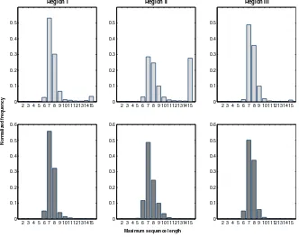
Fig. 6. Acapulco station. Histograms of the maximum sequence length up to whichCEis well-defined for the three epoch regions described in the text, corresponding to the original (top row) and to the shuffled data (bottom row).
Moreover, in order to assess the effect of the data shuffling on theCEcalculation, we obtain the distribution of the
maximum sequence length for which theCEis well-defined (for which there is pattern synchrony), in each calculation
window. In other words, for each calculation window we obtain the value of the longest data-points sequence (pattern) for which there is pattern synchrony, such that for longer sequences the value ofCEis not well-defined. In order to quantify the
difference between the histograms obtained for the original and shuffled data sets, we use the kurtosis (denoted byk) and the skewness (denoted bys) of the distribution of the maximum sequence length.
InFig. 6we see that for region I the histograms for the original and for the shuffled data are similar, withk
=
7.
00 and s=
2.
32, andk=
6.
94 ands=
2.
32; respectively. In both cases, the majority of the calculation windows show the presence of pattern synchrony for sequences up to 7 data-points, although for the original data we observe that there are calculation windows for which the pattern synchrony is present for longer sequences. This suggests that the pattern synchrony between the channels in this region resembles the one exhibited by white noise-like signals. This result is connected to previous works [20,21], in which we have found that for region I the signals in each channel exhibit a variability and correlation profile similar to the one for white noise.On the other hand, we observe more variability in theCEprofile for region II. In particular, notice the significant variation
of theCEthat occurred between January and April 1995. Also, notice that there is certain variability of theCEprofile towards
the end the region. Moreover, the histogram for the maximum sequence length for the data is remarkably different to the one for the shuffled data (seeFig. 6). For the original data the pattern synchrony is present for longer patterns than in the other two regions and there is a significant number of windows for which the pattern synchrony is present for sequences with the maximum length considered, and the histogram hask
=
2.
75 ands=
1.
25. Once the data has been shuffled, the corresponding histogram, withk=
6.
85 ands=
2.
20, exhibits a shape similar to the histograms for the shuffled data of the other regions. From our previous studies on correlations and variability for the signals in separate channels [20,21], the geoelectrical signals for region II exhibit long-range correlation behavior; and the present results suggest that not only the channel signals individually exhibit long-range correlations, but also there is pattern synchrony between channels that persists longer than for the other regions.Finally, for region III we observe that the histogram for the original data is not as similar to that corresponding to the shuffled data as occurs for region I; since the histogram for the original data hask
=
5.
58 ands=
2.
05; while for the shuffled data hask=
5.
64 ands=
2.
08.4.1.3. Coyuca data
TheCEresults for the geoelectrical signals collected by the Coyuca monitoring station are shown inFig. 7, while the
Sequence length
Jun–94 Nov–94 Feb–95 May–95 Aug–95 Nov–95 Feb–96 May–96
Jun–94 Nov–94 Feb–95 May–95 Aug–95 Nov–95 Feb–96 May–96 2
4 6 8 10 12 14
Sequence length
2 4 6 8 10 12 14
[image:9.544.91.451.72.392.2]–0.5 0 0.5 1 1.5 2 2.5 3 3.5 4 Region I Region II Region III
Fig. 7. Cross Sample Entropy analysis for geoelectrical time series from the Coyuca station: Original (top) and shuffled data (bottom).
We observe regularity in theCEprofile for region I. As can be seen inFig. 8, the histogram for the original data is wider
than for the shuffled data, indicating that the pattern synchrony for the original data is defined for longer sequences. The histogram for the original data hask
=
4.
22 ands=
1.
58; while for the shuffled data hask=
7.
75 ands=
2.
40. Notice that the original data from Coyuca in region I exhibits pattern synchrony for longer sequences than for the Acapulco station, where theCEprofile for the original data resembles the one obtained for the shuffled data.On the other hand, for region II we notice the significant variation of theCEthat occurs mainly between April and June
1995. Moreover, the variability ofCEcontinues for the remaining part of the region. Comparing to the results for the Acapulco station (seeFig. 5), it can be seen that this signature occurred later for the Coyuca station, which was farther away from the EQ epicenter than Acapulco. Moreover, from the histogram for the original data in region II we observe that theCEis
well-defined for long sequences for most calculation windows, with a significant number of cases for sequences with 15 samples; showing that the pattern synchrony between the channels in this region persists for long sequences, which is consistent with the observed behavior for the Acapulco data. Moreover, the histogram for the shuffled data is narrower than for the original data. The histogram for the original data hask
=
3.
58 ands=
1.
36; and the one for the shuffled data hask=
6.
79 and s=
2.
18.Finally, for region III we see that theCEprofile at the beginning of the region shows pattern synchrony for long sequences,
with some gaps towards the middle and the end of the region, on which theCEis defined for shorter sequences. Again, we
observe that theCE profile for the shuffled data still shows pattern synchrony on a non-negligible number of cases for
relatively long sequences, with a more even distribution. The variability in theCEprofile in this region is captured by the
histograms shown inFig. 8, on which we observe that after the shuffling, most of the calculation windows give positive values ofCEfor sequences of 7 and 8 samples. Comparing to the results from Acapulco, for the Coyuca station we observe
2 3 4 5 6 7 8 9 101112131415 0
0.1 0.2 0.3 0.4 0.5
Region I
Normalized frequency
2 3 4 5 6 7 8 9 101112131415 0
0.1 0.2 0.3 0.4 0.5
Region II
2 3 4 5 6 7 8 9 101112131415 0
0.1 0.2 0.3 0.4 0.5
Region III
2 3 4 5 6 7 8 9 101112131415 0
0.1 0.2 0.3 0.4 0.5 0.6
2 3 4 5 6 7 8 9 101112131415 0
0.1 0.2 0.3 0.4 0.5 0.6
Maximum sequence length
2 3 4 5 6 7 8 9 101112131415 0
[image:10.544.108.443.54.318.2]0.1 0.2 0.3 0.4 0.5 0.6
Fig. 8. Coyuca station. Histograms of the maximum sequence length up to which theCEis well-defined for the three epoch regions described in the text, corresponding to the original (top row) and to the shuffled data (bottom row).
4.2. Multiscale Cross Entropy results
4.2.1. Simulated signals
We generate signals with 215samples with spectral exponents of
β
=
0, 0.5 and 1.0. The Multiscale Cross Entropy (MCE)
was calculated for sequence lengths up to 12 samples, with tolerancer
=
0.
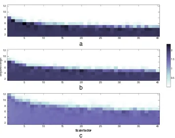
2 and scale factors up to 40.Fig. 9shows the average for ten independent realizations for each value ofβ
. As can be seen for the three signals, theMCEis well-definedeven for large scales, but for increasing sequence lengths as
β
approaches to one. This suggests that signals with long-range correlations exhibit pattern synchrony for longer sequences and in different scales.Notice that for large scales, theMCEfor the three signals shown inFig. 9seems to reach a stable value. For the case of the
white noise, this result may seem counter-intuitive. One thing that should be taken into consideration is that the calculation ofMCEcomprises a moving-average filter operation, therefore, for large scales more points are considered in the filtering
window; which results in having a smoother version of the signal (reduced variability), and therefore the probability to find similar sequences, within the tolerancer, does not vanish but reaches a stable value. This implies that the statistics is poorer as larger scales are considered, since the subseries for the coarse-graining procedure have less data points [5,45].
4.2.2. Geoelectrical signals
The Multiscale Cross Entropy was calculated for the geoelectrical signals for sequence lengths up to 15 samples, with tolerancer
=
0.
2 and for 40 scales. Since a typical file for an observation period of one month has around 1 million records for the Acapulco station, and around half of this for Coyuca (due to the difference in the sampling rate), we split the data files in non-overlapping calculation windows of 42 300 samples for Acapulco and 21 600 samples for Coyuca, corresponding to a 24 h period for each station.For each calculation window a surface is obtained whose height gives the value of theMCE, while thexandyaxes represent
the scale factors and the sequence length, respectively. However, since there are several windows for each month of data, displaying the whole set of results is a difficult task for the present work. Therefore, we select to show the results for some selected scales: 5, 10, 20 and 30; for both the original and shuffled data from the two stations.
Fig. 10shows theMCEanalysis results for the selected scales of the geoelectrical signals, and its shuffled version, from
Acapulco station. Notice that theMCEprofile for region II shows pattern synchrony for longer sequences and for larger scales
than in the other regions, whereMCE profiles are similar to the results obtained for simulated signals with short-range
5 10 15 20 25 30 35 40 2
4 6 8 10
Sequence length
5 10 15 20 25 30 35 40
2 4 6 8 10 12
Scale factor
5 10 15 20 25 30 35 40
2 4 6 8 10 12
0.5 1 1.5 2
a
b
[image:11.544.94.449.44.324.2]c
Fig. 9. Multiscale cross entropy analysis for three different simulated signals with power-law spectral density 1/fβ, withβequal to (a) 0.0, (b) 0.5, and (c) 1.0. Notice that for signals with long-range correlations the pattern synchrony exists for increasing sequence lengths and for large scales.
On the other hand,Fig. 11shows the results of theMCEanalysis of the data from Coyuca station. As can be seen, there is a
higher variability in theMCEprofiles than for Acapulco data; showing the presence of multiscale pattern synchrony for the
three regions, but more significantly for region II. Moreover, the results for the shuffled data show that the shuffling process has significantly destroyed the pattern synchrony for different scales.
5. Discussion
Regarding the variation in theCEprofile for region II for the Acapulco data that occurred between January and April 1995
(seeFig. 5), it could have been related to the occurrence of theM
=
7.
4 EQ on September 14, 1995. On the other hand, the pattern synchrony profile for region II for Coyuca data shows a noticeable variability starting on April 1995 and that extends to the remaining part of the region and to region III as well (seeFig. 7). One thing to notice is that this signature did not occur immediately before the EQ, in fact, it was observed several months earlier. A similar result was reported in Ref. [29], when performing spectral analysis on the signals from the same monitoring stations. According to this study, the electric activity observed by each monitoring station is neither the same nor simultaneous, but the bursts propagate through the crust with an intensity that depends on the distance from the EQ epicenter to the detector, on the electrical properties of the soil at the monitoring station as well as on the properties of the medium between the EQ epicenter and the detector [29]. Moreover, independent studies [49,50] have shown that the SES amplitude recorded at a given measuring station depends on the inhomogeneities around the station as well as on the geoelectrical structure, in general, of the medium between the EQ epicenter and the station.Moreover, it can be seen that this signature occurred later for the Coyuca station, which was farther away from the EQ epicenter than Acapulco. This result is consistent with that reported in Ref. [29], in which it was suggested that the electric pulses are generated by local effects in the sites of the stations, perhaps correlated to a kind of stress pulses traveling away from the epicentral region; and therefore these signals appear earlier at the closest monitoring station. In fact, in Ref. [29] it was estimated that for the geological zone here considered, the traveling stress pulse has an apparent speed of 1–2 km/day. However, in Ref. [29] true electric anomalies were considered which were evaluated through the integral of the spectral density function for each channel. Nevertheless, in the present work we are calculating the pattern synchrony between orthogonal channels, which provides information about the pattern similarity between the signals from each channel.
Sequence length Sequence length
Sequence length Sequence length
2 4 6 8 10 12 14 2 4 6 8 10 12 14 2 4 6 8 10 12 14 2 4 6 8 10 12 14 2 4 6 8 10 12 14 2 4 6 8 10 12 14 0 1 2 3 0 1 2 3 4 0 1 2 3 4 5 6 0 1 2 3
Region I Region II Region III Region I Region II Region III
Shuffled Shuffled Shuffled Shuffled 2 4 6 8 10 12 14
Jun–94 Aug–94 Nov–94 Feb–95 May–95 Aug–95 Nov–95 Feb–96 May–96 Jun–94 Aug–94 Nov–94 Feb–95 May–95 Aug–95 Nov–95 Feb–96 May–96
Jun–94 Aug–94 Nov–94 Feb–95 May–95 Aug–95 Nov–95 Feb–96 May–96 Jun–94 Aug–94 Nov–94 Feb–95 May–95 Aug–95 Nov–95 Feb–96 May–96
[image:12.544.66.485.57.357.2]–0.5 0 0.5 1 1.5 2 2.5 3 –0.5 0 0.5 1 1.5 2 2.5 3 –0.5 0 0.5 1 1.5 2 2.5 3 0 1 2 3 4 5
a
b
c
d
2 4 6 8 10 12 14Fig. 10. Multiscale cross entropy analysis of geoelectrical time series, and its shuffled version, from the Acapulco station for selected scales: (a) 5, (b) 10, (c) 20 and (d) 30.
fluctuations of the electric field (the background noise), the pattern synchrony between the channels is not sustained for long sequences, resembling the results for the white noise. However, when the source of the electric field is relatively far away from the electrodes, perhaps associated with a regional zone affected by a certain excitation caused by a seismic front traveling from the focal zone, such as was reported in Ref. [29], the pattern synchrony between the channels persists for longer sequences. Therefore, the pattern synchrony is a possible expression of a dominant regional field mounted over the local background noise.
Moreover, the results from the multiscale cross entropy analysis (seeFigs. 10and11) for data in region II from both stations indicate that the pattern synchrony persists for long sequences and large scales. In a previous work [20], we found that for the data in region II, each channel exhibited a correlated behavior when applying the multiscale entropy analysis. Our present results indicate that, in addition to the appearance of correlated dynamics in each channel, it is observed that pattern synchrony between the channels persists for other scales. As can be seen, the results of the multiscale pattern synchrony for both stations differ between each other, for the reasons discussed previously for the single scale pattern synchrony.
The present results are consistent with those deduced by analyzing the time-series in a new time domain termed natural time [6,7]: when analyzing the original time series of SES activities, the entropyS defined in natural time [51] and the entropyS−upon time reversal are obtained; then [27] both values (S andS−) are found to be smaller than the entropy
calculated for the shuffled data. This comes from the fact that, since SES activities are characterized by critical dynamics, they exhibit infinitely ranged temporal correlations [9], which are however destroyed upon randomly shuffling the original data. Moreover the fact that the entropy of the shuffled data is found to be equal to that of auniformdistribution (white noise), reveals that the self-similarity of SES activities stems solely from long-range temporal correlations, i.e., from the process memory only (and not from the process’ incrementsinfinitevariance, see Ref. [28] for details).
6. Conclusions
The contribution of this work is the introduction of the Cross Sample Entropy (CE) analysis to the study of electrical
signals related to earthquake activity, which to our best knowledge has not been applied to these kind of signals. TheCE
analysis gives information about thepattern synchronybetween two signals. We calculate theCEprofile between the NS
Sequence length
Region I Region II Region III Region I Region II Region III
Sequence length Sequence length
Sequence length 2 4 6 8 10 12 14
Jun–94 Nov–94 Feb–95 May–95 Aug–95 Nov–95 Feb–96 May–96 Jun–94 Nov–94 Feb–95 May–95 Aug–95 Nov–95 Feb–96 May–96
Jun–94 Nov–94 Feb–95 May–95 Aug–95 Nov–95 Feb–96 May–96
Jun–94 Nov–94 Feb–95 May–95 Aug–95 Nov–95 Feb–96 May–96
[image:13.544.67.479.56.348.2]2 4 6 8 10 12 14 2 4 6 8 10 12 14 2 4 6 8 10 12 14 0 1 2 3 0 1 2 3 4 0 1 2 3 0 1 2 3 4 5 0 1 2 3 0 1 2 3 4 5 0 1 2 3 4 5 6 Shuffled Shuffled Shuffled Shuffled
a
b
c
d
–0.5 0 0.5 1 1.5 2 2.5 3 2 4 6 8 10 12 14 2 4 6 8 10 12 14 2 4 6 8 10 12 14 2 4 6 8 10 12 14Fig. 11. Multiscale cross entropy analysis of geoelectrical time series, and its shuffled version, from the Coyuca station for selected scales: (a) 5, (b) 10, (c) 20 and (d) 30.
sustained for relatively large patterns. This behavior was observed for simulated signals with long-range correlations. In addition, we observed that there are periods for which theCEprofile for the data is very similar to the one obtained for
the shuffled data; which in turn resembles the one obtained for simulated signals with short-range correlations. Moreover, when the orthogonal electrodes measure only very local random fluctuations of the electric field (the local background noise), the pattern synchrony between the channels is not sustained for long sequences, resembling the results of white noise. However, when the traveling stress front arrives at the local region of each station, the electric field relatively far away from the electrodes, the pattern synchrony between the channels persists for longer sequences. Therefore, the pattern synchrony is a possible expression of a dominant relatively far field mounted over the very local background noise.
On the other hand, we have extended the Multiscale Entropy method to include the calculation of the cross entropy between the signals in both channels, which represents a novel approach to the study of the pattern synchrony between two signals. Moreover, the Multiscale Cross Entropy (MCE) profile observed for the data close to the occurrence of aM
=
7.
4EQ shows that the pattern synchrony persists for long sequences and different scales. In addition, we notice that the behavior of theMCEprofile for data from epoch regions far from the EQ occurrence is similar to the results obtained for simulated
signals with short-range correlations. Nevertheless, more work should be performed to improve the interpretation and applicability of this tool for the study of multiscale pattern synchrony for time series in different research fields, such as for physiological signals.
Results from previous works based on the study of correlations and variability concluded that in the vicinity of an EQ the geoelectrical signals individually exhibit a complex behavior [11,20,21]. Our results suggest that, in addition to this, the signals exhibit pattern synchrony between channels for long sequences and through multiple scales.
Acknowledgements
This work was partially supported by CONACYT (Grant 49128-F-26020), COFAA-IPN, EDI-IPN, México. The authors wish to thank to the referees whose suggestions allowed the improvement of this manuscript.
References
[1] S.M. Pincus, Approximate entropy as a measure of system complexity, Proc. Natl. Acad. Sci. 88 (1991) 2297–2301. [2] S.M. Pincus, Approximate entropy (ApEn) as a complexity measure, Chaos 5 (1995) 110–117.
[4] A.L. Goldberger, C.K. Peng, L.A. Lipsitz, What is physiologic complexity and how does it change with aging and disease? Neurobiol. Aging 23 (2002) 23–26.
[5] M. Costa, A.L. Goldberger, C.K. Peng, Multiscale entropy analysis of physiologic time series, Phys. Rev. E 98 (2002) 062102.
[6] P.A. Varotsos, N.V. Sarlis, E.S. Skordas, Long-range correlations in the electric signals that precede rupture, Phys. Rev. E 66 (2002) 011902.
[7] P.A. Varotsos, N.V. Sarlis, E.S. Skordas, Long-range correlations in the electric signals that precede rupture: Further investigations, Phys. Rev. E 67 (2003) 021109.
[8] P.A. Varotsos, N.V. Sarlis, H.K. Tanaka, E.S. Skordas, Similarity of fluctuations in correlated systems: The case of seismicity, Phys. Rev. E 72 (2005) 041103.
[9] P.A. Varotsos, N.V. Sarlis, E.S. Skordas, H.K. Tanaka, M.S. Lazaridou, Entropy of seismic electric signals: Analysis in natural time under time reversal, Phys. Rev. E 73 (2006) 031114.
[10] F. Angulo-Brown, A. Muñoz-Diosdado, Further seismic properties of a spring-block earthquake model, Geophys. J. Int. 139 (1999) 410–418. [11] A. Ramírez-Rojas, C.G. Pavía-Miller, F. Angulo-Brown, Statistical behavior of the spectral exponent and the correlation time of electric self-potential
time series associated to theMs=7.4 September 14, 1995 earthquake in Mexico, Phys. Chem. Earth 29 (2004) 305–312.
[12] A. Ramírez-Rojas, A. Muñoz-Diosdado, C.G. Pavía-Miller, F. Angulo-Brown, Spectral and multifractal study of electroseismic time series associated to theMw=6.5 earthquake of 24 October 1993 in Mexico, Nat. Hazards Earth Syst. Sci. 4 (2004) 703–709.
[13] L. Telesca, V. Lapenna, M. Lovallo, Fisher information measure of geoelectrical signals, Physica A 351 (2005) 637–644. [14] L. Telesca, V. Lapenna, M. Macchiato, Multifractal fluctuations in seismic interspike series, Physica A 354 (2005) 629–640.
[15] L. Telesca, V. Cuomo, M. Lanfredi, V. Lapenna, M. Macchiato, Investigating clustering structures in time-occurrence sequences of seismic events observed in the Irpinia-Basilicata region (southern Italy), Fractals 7 (1999) 221–234.
[16] L. Telesca, V. Cuomo, V. Lapenna, F. Vallianatos, Self-similarity properties of seismicity in the Southern Aegean area, Tectonophysics 321 (2000) 179–188.
[17] L. Telesca, V. Cuomo, V. Lapenna, M. Macchiato, Analysis of the time-scaling behaviour in the sequence of the aftershocks of the Bovec (Slovenia) April 12, 1998 earthquake, Phys. Earth Planet. Inter. 120 (2000) 315–326.
[18] L. Telesca, V. Lapenna, M. Macchiato, Investigating the time-clustering properties in seismicity of Umbria-Marche region (central Italy), Chaos Solitons Fractals 18 (2003) 203–217.
[19] L. Telesca, V. Cuomo, V. Lapenna, M. Macchiato, Detrended fluctuation analysis of the spatial variability of the temporal distribution of Southern California seismicity, Chaos Solitons Fractals 21 (2004) 335–342.
[20] L. Guzmán-Vargas, A. Ramírez-Rojas, F. Angulo-Brown, Multiscale entropy analysis of electroseismic time series, Nat. Hazards Earth Syst. Sci. 8 (2008) 855–860.
[21] L. Guzmán-Vargas, A. Ramírez-Rojas, R. Hernández-Pérez, F. Angulo-Brown, Correlations and variability in electrical signals related to earthquake activity, Physica A 388 (2009) 4218–4228.
[22] V. Cuomo, V. Lapenna, M. Macchiato, C. Serio, L. Telesca, Stochastic behaviour and scaling laws in geoelectrical signals measured in a seismic area of southern Italy, Geophys. J. Int. 139 (1999) 889–894.
[23] G. Ouillon, D. Sornette, E. Ribeiro, Multifractal Omori law for earthquake triggering: New tests on the California, Japan and worldwide catalogues, Geophys. J. Int. 178 (2009) 215–243.
[24] M. Hayakawa, T. Ito, N. Smirnova, Fractal analysis of ULF geomagnetic data associated with the Guam Earthquake on August 8, 1993, Geophys. Res. Lett. 26 (18) (1999) 2797–2800.
[25] P.A. Varotsos, K. Alexopoulos, Physical properties of the variations of the electric field of the Earth preceding earthquakes I, Tectonophysics 110 (1984) 73–98.
[26] P.A. Varotsos, K. Alexopoulos, Physical properties of the variations of the electric field of the Earth preceding earthquakes II, Tectonophysics 110 (1984) 99–125.
[27] P.A. Varotsos, N.V. Sarlis, H.K. Tanaka, E.S. Skordas, Some properties of the entropy in the natural time, Phys. Rev. E 71 (2005) 032102.
[28] P.A. Varotsos, N.V. Sarlis, E.S. Skordas, H.K. Tanaka, M.S. Lazaridou, Attempt to distinguish long-range temporal correlations from the statistics of the increments by natural time analysis, Phys. Rev. E 74 (2006) 021123.
[29] E. Yépez, J.G. Pineda, J.A. Peralta, A.V. Porta, C.G. Pavía-Miller, F. Angulo-Brown, Spectral analysis of ULF electric signals possibly associated to earthquakes, in: M. Hayakawa (Ed.), Atmospheric and Ionospheric Electromagnetic Phenomena Associated with Earthquakes, Terra Scientific Publishing Company, Tokyo, 1999, pp. 115–121.
[30] L. Telesca, G. Colangelo, V. Lapenna, Multifractal variability in geoelectrical signals and correlations with seismicity: A study case in southern Italy, Nat. Hazards Earth Syst. Sci. 5 (2005) 673–677.
[31] J.R. Luévano, A. Ramírez-Rojas, Mutual information statistics for electroseismic time series, Geophys. Res. Abstr. 8 (2006) 01576.
[32] A. Ramírez-Rojas, E.L. Flores-Márquez, L. Guzmán-Vargas, J. Márquez-Cruz, C.G. Pavía-Miller, F. Angulo-Brown, A comparison of ground geoelectric activity between three regions of different level of seismicity, Nat. Hazards Earth Syst. Sci. 7 (2007) 591–598.
[33] E.L. Flores-Márquez, J. Márquez-Cruz, A. Ramírez-Rojas, G. Gálvez-Coyt, F. Angulo-Brown, A statistical analysis of electric self-potential time series associated to two 1993 earthquakes in México, Nat. Hazards Earth Syst. Sci. 7 (2007) 549–556.
[34] A. Ramírez-Rojas, E.L. Flores-Márquez, J. Márquez-Cruz, L. Guzmán-Vargas, G. Gálvez-Coyt, L. Telesca, F. Angulo-Brown, Statistical features of electroseismic signals prior to M7.4 Guerrero–Oaxaca earthquake (México), Nat. Hazards Earth Syst. Sci. 8 (2008) 1001–1007.
[35] J. Richman, J. Moorman, Physiological time-series analysis using approximate entropy and sample entropy, Am. J. Physiol. Heart Circ. Physiol. 278 (2000) H2039–H2049.
[36] S.M. Pincus, T. Mulligan, A. Iranmanesh, S. Gheorghiu, M. Godschalk, J.D. Veldhuis, Older males secrete luteinizing hormone and testosterone more irregularly, and jointly more asynchronously, than younger males, Proc. Natl. Acad. Sci. 93 (1996) 14100–14105.
[37] J.D. Veldhuis, A. Iranmanesh, T. Mulligan, S.M. Pincus, Disruption of the young–adult synchrony between luteinizing hormone release and oscillations in Follicle-Stimulating Hormone, Prolactin, and Nocturnal Penile Tumescence (NPT) in healthy older men, J. Clin. Endocrinol Metab. 84 (1999) 3498–3505.
[38] P.Y. Liu, S.M. Pincus, D.M. Keenan, F. Roelfsema, J.D. Veldhuis, Analysis of bidirectional pattern synchrony of concentration–secretion pairs: Implementation in the human testicular and adrenal axes, Am. J. Physiol. Regul. Integr. Comp. Physiol. 288 (2005) 440–446.
[39] T. Kuusela, T. Jartti, K. Tahvanainen, T. Kaila, Nonlinear methods of biosignal analysis in assessing terbutaline-induced heart rate and blood pressure changes, Am. J. Physiol. Heart Circ. Physiol. 282 (2002) 773–781.
[40] Z. Hu, P. Shi, Interregional functional connectivity via pattern synchrony, in: Proceedings of the Ninth International Conference on Control, Automation, Robotics and Vision, IEEE, 2006, pp. 1–6.
[41] T. Zhang, Z. Yang, J.H. Coote, Cross-sample entropy statistic as a measure of complexity and regularity of renal sympathetic nerve activity in the rat, Experiment. Phys. 94 (2007) 659–669.
[42] P. Grassberger, I. Procaccia, Estimation of the Kolmogorov entropy from a chaotic signal, Phys. Rev. A 28 (1983) 2591–2593. [43] J.P. Eckmann, D. Ruelle, Ergodic theory of chaos and strange attractors, Rev. Modern Phys. 57 (1985) 617–656.
[44] S. Pincus, B.H. Singer, Randomness and degrees of irregularity, Proc. Natl. Acad. Sci. 93 (1996) 2083–2088. [45] M. Costa, A.L. Goldberger, C.K. Peng, Multiscale entropy analysis of biological signals, Phys. Rev. E 71 (2005) 021906.
[46] E. Yépez, F. Angulo-Brown, J.A. Peralta, C.G. Pavía-Miller, G. González-Santos, Electric fields patterns as seismic precursors, Geophys. Res. Lett. 22 (1995) 3087–3090.
[47] H.-O. Peitgen, D. Saupe, The Science of Fractal Images, Springer, New York, 1988.
[48] V. Paxson, Fast, approximate synthesis of fractional Gaussian noise for generating self-similar network traffic, ACM Comput. Commun. Rev. 27 (1997) 5–18.
[49] P. Varotsos, M. Lazaridou, Latest aspects of earthquake prediction in Greece based on seismic electric signals I, Tectonophysics 188 (1991) 321–347. [50] P. Varotsos, K. Alexopoulos, M. Lazaridou, Latest aspects of earthquake prediction in Greece based on seismic electric signals II, Tectonophysics 224
(1993) 1–37.
![Fig. 1. A simulated time seriesA u[1], . . . , u[N] is shown to illustrate the procedure for finding sequence matches to calculate the Approximate (AE) andSample (SE) entropies for the case m = 2 and a given tolerance r (a fraction of the standard deviatio](https://thumb-us.123doks.com/thumbv2/123dok_es/5523478.118235/3.544.130.413.53.281/simulated-illustrate-procedure-calculate-approximate-andsample-entropies-tolerance.webp)


![Fig. 4. Cross Sample Entropy analysis for synthetic 1/f β-signals, with β ∈ [0, 1]. (a) Shows the CE between two signals with the same β; while the figuresat the right show the results of CE between signals with different spectral exponents β1 and β2, for the sequence lengths of (b) 5, (c) 10, and (d) 15 samples.](https://thumb-us.123doks.com/thumbv2/123dok_es/5523478.118235/7.544.90.450.362.672/entropy-analysis-synthetic-figuresat-different-spectral-exponents-sequence.webp)