T
HEA
NATOMY OF AM
ULTIPLEC
RISIS:
W
HY WASA
RGENTINA SPECIAL AND WHAT CAN WE LEARN FROM IT 1DRAFT
Guillermo Perry and Luis Servén
Chief Economist Office, LAC
The World Bank
This version: May10, 2002
I. INTRODUCTION AND SUMMARY:
II. ECONOMIC PERFORMANCE AND EXTERNAL SHOCKS The Endogeneity of Capital Flow Reversals
III. OVERVALUATION AND DEFLATIONARY ADJUSTMENT UNDER THE HARD PEG :
Why Old Lessons about Optimal Currency Areas should not be Forgotten. IV. FISCAL VULNERABILITIES:
Mismanagement in the Boom and large Fiscal Contingencies associated with adverse external shocks
V. THE BANKING SYSTEM:
Vulnerabilities behind a strong façade. VI. POLICY DILEMMAS AND OPTIONS:
The lost opportunities in the boom years.
I INTRODUCTION AND SUMMARY
The severity of the Argentine Crisis and its dire social cost have come as a surprise to most observers, even to those that had been predicting it since the Brazilian devaluation of 1999. There were very few that predicted it before 1999. Indeed, the Argentine economy appeared to be in relatively good shape at least until before the Russian crisis. Even then the attention of the markets and the International Financial Institutions was focused on Brazil, which had more apparent macroeconomic imbalances and had suffered severe speculative attacks in October 1997 and again after the Russian crisis, leading to the demise of the exchange rate band and a sharp devaluation of the Real in January 1999.
Argentina outperformed most other economies in the region until 1997 in terms of growth per capita -- though income distribution did not improve and unemployment stayed at high levels -- in a relatively benign external environment (terms of trade, capital inflows and spreads, world growth), in spite of a short-lived interruption in 1995 when it suffered severe contagion from the so-called Tequila crisis. But after the major slowdown in growth in 1999 that affected the whole region, mainly due to capital flow retrenchment after the Russian crisis, other countries in the region began a modest recovery, while Argentina plunged into a protracted recession, reversing most of her previous gains at poverty reduction. We explore in Section II if this difference in performance can be attributed to Argentina receiving more severe external shocks than other economies in the region. We find that Argentina was not hit harder than other Latin American countries by the terms of trade decline after the Asian crisis, nor by the US and worldwide slowdown in 2001, nor by the capital flows reversal and the rise in spreads after the Russian crisis. As a consequence, the fact that Argentina did worse than other countries after 1999 must be attributed to her higher vulnerabilities to shocks, weaker policy responses or a combination of both. Indeed, we find in Section II that the large capital flow reversal in 2001 was driven by Argentina-specific factors. We view this as evidence that “sudden stops” of capital flows acted more as an amplifier than as a primary cause of the crisis 2.
Thus, the bulk of this paper is devoted to examine to which extent and why was the Argentine economy more vulnerable to adverse external shocks than other Latin American economies, and to what extent were policy mistakes (particularly during the De la Rua Government) the main culprit, as is often claimed. We examine the vulnerabilities associated with deflationary adjustments to shocks under a hard peg in Section III; those associated with a large public debt and a fragile fiscal position in Section IV and those hidden under a façade of strength in the banking sector in Section V. We conclude that although there were important vulnerabilities in each of these areas, neither of them on its own was larger than those affecting some other countries in the region, and thus there is no one obvious suspect. However, we also find that they reinforced each other in such a perverse way that taken jointly they led to a much larger vulnerability to adverse external shocks than in any other country in the region.
In particular, the hard peg and inflexible domestic nominal wages and prices imposed a protracted deflationary adjustment in response to the depreciation of the Euro and the real, the terms of trade shocks and the capital market shock of 1998, leading to a major overvaluation of the currency and a rapidly deteriorating net foreign asset position. Such imbalances were aggravated by weak fiscal policies during the decade, especially after 1995. In Section III we estimate that all these factors led since 1997 to an increasing overvaluation of the currency that peaked in 2001 at about 55%. The need to address the rising concern with solvency – given the large debt, the weak primary fiscal balance and low growth – led to tax hikes and budget cuts in 2000 and 2001 that deepened the economic contraction. The endogenous capital flow reversal and increased risk premium in 2001 amplified these problems by requiring a large external current account adjustment. To aggravate matters, such an adjustment under the hard peg had to take place mostly through demand reduction and aggregate deflation – a lengthy, costly and uncertain process.
The hard peg actually hid from public view the serious deterioration in fiscal solvency and the mounting financial stress. Indeed, the protracted deflationary adjustment required to realign the real exchange rate under the hard peg would have unavoidably eroded the debt repayment capacity of the Government, households and firms in non tradable sectors – the debtors whose incomes would be more adversely affected as a direct result of the deflation.3 The nominal devaluation in 2002 revealed in full force
these latent problems and made them much worse due to the exchange rate overshooting and the disruption of the payments system derived from the deposit freeze (the so called “corralito”) -- which might have been partially avoided by better policy responses. Financial stress was aggravated by the large exposure of banks and Pension Funds to increasing Government risk. Thus a vicious circle of economic contraction, fiscal hardship and financial stress ensued.
The authorities and the Argentine polity were indeed faced with very harsh dilemmas after 1998 (as discussed in Section VI). They were placed between a rock and a hard place. One option was to accept a painful and protracted deflationary adjustment while keeping the Currency Board – and attempting to retain market confidence in the meantime. This would have entailed a severe test of the fragile Argentine political and fiscal institutions. An early adoption of full dollarization might have reduced the pains and duration of the deflationary adjustment and thus increased the likelihood of success of such an option.
The other option was to allow a nominal devaluation and adopt a float, in an attempt to shortcut the protracted deflationary adjustment. However, this would have precipitated a latent corporate, banking and fiscal crisis, given the open currency exposures in the balance sheets of both the public and the private sectors and the large degree of overvaluation of the currency. In order to avoid such scenario, financial contracts would have to be pesified before floating. But this in turn posed the serious
danger of a deposit run, which would have forced a deposit freeze and/or some kind of Bonex plan, fatally eroding the public’s confidence in money as a store of value. In the event, the authorities did not use well their limited margin of maneuver, by engaging in too little and too late fiscal adjustment (which actually should have been done in the boom years before 1999), by hesitating on the ultimate choice of exchange rate regime, by postponing too long the needed public debt restructuring, and by precipitating a major financial and payments crisis – first reducing the liquidity buffers of the banking system and over-exposing it (as well as the Pension Funds) to Government risk, and later adopting an arbitrary asymmetric pesification of assets and liabilities and a particularly disruptive deposit freeze, which was held for an excessively long period of time without resolution. Such measures and omissions aggravated the depth of the crisis and created additional unnecessary problems for the recovery.
These hard choices were a reflection of a deep structural problem. On the one hand, the Argentine trade structure made a peg to the dollar highly inadequate -- from a real economy point of view. On the other hand, the strong preference of Argentineans for the dollar as a store of value (since the hyperinflation and confiscation experiences of the 1980s) had led to a highly dollarized economy in which a hard peg or even full dollarization seemed a reasonable alternative – from a financial point of view. No wonder that informed analysts favored –and still do- opposite exchange regime choices depending on the relative weight they assign to real economy or financial (balance sheet) effects.
With the benefit of hindsight the boom years up to mid 1998 were a major lost opportunity. Staying with the hard peg but minimizing the risks associated with adverse external shocks would have required: (1) First and foremost, significant fiscal strengthening, not just to protect solvency but with the broader objective of providing some room for counter-cyclical fiscal policy. This contrasts with the expansionary pro-cyclical stance actually followed during most of the decade, and especially during the boom from end-1995 up to mid-1998 – once the implicit pension debt (as well as other implicit liabilities) had been brought in the open by pension reform (as documented in Section IV). (2) Second, considerable flexibilization of labor and other domestic markets (including utilities). (3) Third, significant unilateral opening to trade. None of this was done in the nineties. And (4) Fourth, even stricter prudential regulations for banks than actually adopted (in spite of the significant progress in this field), probably leading to a form of narrow banking, harder provisioning and/or capital requirements to lend to households and firms in non tradable sectors and a “firewall” between banks and the Government (as discussed in Section V).
Just too often in Latin America the seeds of crisis are planted in good times by imprudent behavior or lack of precautionary action whose consequences are only revealed when bad times arrive. There are deep political economy factors that help to explain such bad outcomes. A key lesson from Argentina is the need to adopt economic and political institutions that align incentives to face hard choices and facilitate timely reforms, and in particular that are less prone to amplifying economic cycles.
The analysis of the Argentine crisis yields many other useful lessons for other Latin American economies. After all, the exchange rate system dilemma faced by a highly dollarized economy that conducts only a fraction of its trade with the US, in a world economy characterized by highly volatile currencies, is not exclusive to Argentina. But even economies with less stringent structural dilemmas often face some form of tension between the convenience of adopting and maintaining a flexible exchange rate regime with a monetary anchor in order to achieve flexibility in responding to shocks, on the one hand, and balance sheet vulnerabilities to major real exchange rate adjustments originated in unhedged foreign-currency debt of firms in non-tradable sectors and of Governments themselves.4 Even those could draw useful policy lessons from the Argentine debacle. And so can we, in the International Financial Institutions, as we must admit that we were slow in understanding some of the deep problems discussed here and in reacting to them.
II ECONOMIC PERFORMANCE AND EXTERNAL SHOCKS IN THE 90s
Over 1990-97, Argentina outperformed most other economies in the region in terms of growth (Table 2.1). These were years of relatively benign external environment (terms of trade, capital inflows, spreads, and world growth), with a short-lived but abrupt interruption in 1995 due to the Tequila crisis, from which Argentina suffered a severe contagion. The growth performance remained fairly satisfactory even in 1998. But after the region-wide growth slowdown of 1999 – largely a consequence of capital flow retrenchment following the Russian crisis – other Latin American countries began a modest recovery, while Argentina plunged into a protracted recession.
Table 2.1
Real GDP Growth Rate
(Percentages)
1981-90 1991-97 1998 1999 2000-01
Argentina -1.3 6.7 3.9 -3.4 -2.1
Bolivia -0.4 4.3 5.5 0.6 1.5
Brazil 2.3 3.1 0.2 0.8 3.1
Chile 4.0 8.3 3.9 -1.1 4.3
Colombia 3.4 4.0 0.5 -4.3 2.2
Costa Rica 2.4 4.9 8.4 8.2 1.3
Ecuador 2.1 3.2 0.4 -7.3 3.9
Mexico 1.5 2.9 4.9 3.8 3.3
Peru 0.0 5.3 -0.4 1.4 1.9
Venezuela 0.3 3.4 0.2 -6.1 3.3
Average 2.0 3.6 3.2 1.6 2.1
Source: World Development Indicators Database and the Unified Survey.
Unemployment kept a slightly increasing trend up to the Tequila crisis, when it jumped sharply (Figure 2.1). The fact that unemployment was rising even when the economy was growing at full steam reflects a combination of increasing participation rates (probably stemming from an ‘encouragement effect’ due to the growth upturn), productive restructuring towards less labor-intensive activities, and probably also the poor operation of the labor market.5 The unemployment rate declined in the boom years 1996-1998, to resume an upward trend during the ensuing recession.
Poverty indicators display a similar trajectory (Figure 2.1). Poverty declined sharply until 1994, but rose again with the Tequila crisis and then continued on an upward trend during the recession of 1999-2000, so that by 2000 most of the gains at
poverty reduction achieved in the early part of the decade had been wiped out. Even more striking is the trajectory of inequality, which appears to have risen without interruption from 1993 on, after an initial decline in 1990-92.
Figure 2.1
Poverty, Inequality, and Unemployment
41.4
30.4
24.1
21.8 21.6
27.2
30 29.4 29.4 31.51
34.32
7.5 6.5 7
9.6 11.5 17.5 17.2 14.9 12.8 14.2 15.05 0 5 10 15 20 25 30 35 40 45
1990 1991 1992 1993 1994 1995 1996 1997 1998 1999e 2000e
0.43 0.44 0.45 0.46 0.47 0.48 0.49 0.5
Gini Coeficient (Right scale) Unemployment (Left scale)
Data for urban areas. Sources: Unemployment from INDEC, Gini Coeficient and Poverty Head Count Ratio from World Bank Poverty Assesment Report (2000) except for the 1999-2000 ratios which are estimated using the trend observed for the Greater Buenos Aires headcound ratios from INDEC.
Poverty Headcount Ratio (Left scale)
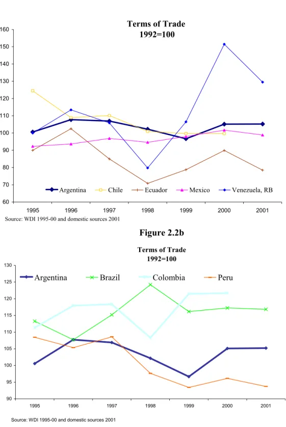
Was Argentina’s poor performance from 1999 onward a reflection of worse external shocks than those affecting other LAC countries? To answer this question, we first consider real shocks – those stemming from terms of trade changes and global growth – and then look at capital flow disturbances.
Figure 2.2a
Terms of Trade 1992=100
60 70 80 90 100 110 120 130 140 150 160
1995 1996 1997 1998 1999 2000 2001
Argentina Chile Ecuador Mexico Venezuela, RB
Source: WDI 1995-00 and domestic sources 2001
Figure 2.2b Terms of Trade
1992=100
90 95 100 105 110 115 120 125 130
1995 1996 1997 1998 1999 2000 2001
Argentina Brazil Colombia Peru
Figure 2.2c
Terms of Trade Shocks (% of GDP)
-8 -6 -4 -2 0 2 4 6 8 10 12 14
1995 1996 1997 1998 1999 2000
Argentina Chile Ecuador Mexico Venezuela, RB
Source: WDI.
Figure 2.2d
Terms of Trade Shocks (% of GDP)
-1.5 -1.0 -0.5 0.0 0.5 1.0 1.5 2.0
1995 1996 1997 1998 1999 2000
Argentina Brazil Colombia Peru
In any case, the economic impact of these gyrations in Argentina’s terms of trade is virtually negligible when compared with other countries. The reason is that Argentina is a fairly closed economy, and thus terms of trade changes entail only modest changes in real income. This is highlighted in Figures 2.2c and 2.2d, which portray the terms of trade
shocks suffered by various LAC economies, defined by multiplying the changes in import
and export prices by the respective magnitudes of imports and exports relative to GDP. It is immediately apparent that Argentina’s terms of trade shocks over the second half of the 1990s were smaller in magnitude than those of any other country in the graphs, perhaps with the only exception of Brazil (which is also fairly closed). Indeed, Argentina’s real income loss from the terms of trade fall in 1998-99 amounted to less than 0.5 percent of GDP.
Table 2.2
The Global Slowdown: Impact on the Region
The Income Effect via Trade Volume
Exports/
GDP (%)
Exports of goods to US/Total Exports
(%)
Impact of expected decline in U.S. growth
(% of GDP)
Impact of import decline in industrialized
countries (% of GDP)
(a) (b) (c)=-[(a)*(b)*0.022]*4.1 (d)=(a)*0.10
Argentina 10.77 11.37 -0.11 -1.08
Bolivia 17.10 33.20 -0.51 -1.71
Brazil 10.88 22.64 -0.22 -1.09
Chile 30.74 18.00 -0.50 -3.07
Colombia 19.03 50.27 -0.86 -1.90
Costa Rica 47.94 51.94 -2.25 -4.79
Dominican Rep. 32.25 12.79 -0.37 -3.23
Ecuador 42.43 38.38 -1.47 -4.24
Guatemala 20.26 34.31 -0.63 -2.03
Jamaica 51.40 32.61 -1.51 -5.14
Mexico 31.85 88.40 -2.54 -3.19
Peru 16.07 29.09 -0.42 -1.61
Venezuela, RB 27.22 51.61 -1.27 -2.72
(a)Exports of Goods and Services and GDP of 2000, source: WDI. (b) Exports of goods in 1999 except 1997 for DR and Jamaica, source:UN_Comtrade.(c) 2.2 is the U.S. expenditure elasticity (Clarida,1994), and 4.1% is the expected decline in the U.S.(d)10 % is the expected decline of imports from industrilized economies.
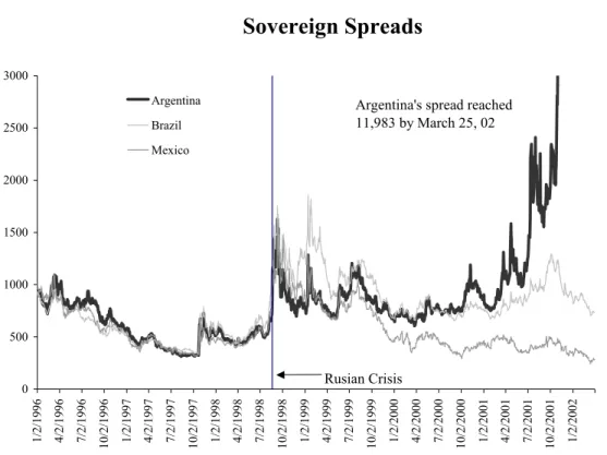
Figure 2.3
Sovereign Spreads
0 500 1000 1500 2000 2500 3000
1/2/1996 4/2/1996 7/2/1996 10/2/1996 1/2/1997 4/2/1997 7/2/1997 10/2/1997 1/2/1998 4/2/1998 7/2/1998 10/2/1998 1/2/1999 4/2/1999 7/2/1999 10/2/1999 1/2/2000 4/2/2000 7/2/2000 10/2/2000 1/2/2001 4/2/2001 7/2/2001 10/2/2001 1/2/2002
Argentina
Brazil
Mexico
Argentina's spread reached 11,983 by March 25, 02
Rusian Crisis
Source: JP Morgan
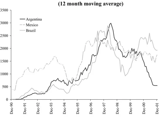
Figure 2.4
Gross Capital Inflows (12 month moving average)
0 500 1000 1500 2000 2500 3000 3500
Dec-90 Dec-91 Dec-92 Dec-93 Dec-94 Dec-95 Dec-96 Dec-97 Dec-98 Dec-99 Dec-00 Dec-01
Argentina Mexico Brazil
Figure 2.5a
Capital Account
(Percentage GDP)
-4 -2 0 2 4 6 8 10 12
1997-IV 1998-I 1998-II 1998-III 1998-IV 1999-I 1999-II 1999-III 1999-V 2000-I 2000-II 2000-III 2000-IV 2001-I 2001-II 2001-III
Argentina
LAC GDP Weighted Mean
Figure 2.5b
Current Account
(Percentage of GDP)
-7 -6 -5 -4 -3 -2 -1 0
1997-IV 1998-I 1998-II 1998-III 1998-IV 1999-I 1999-II 1999-III 1999-V 2000-I 2000-II 2000-III 2000-IV 2001-I 2001-II 2001-III
Argentina
LAC GDP Weighted Mean
Table 2.3
Current Account Deficit Adjustment
1998/99 2000/01e 1998/99 2000/01e
Argentina 0.77 1.27 7.16 14.33
Bolivia 1.44 1.58 4.96 8.00
Brazil 1.11 -0.55 13.83 -7.33
Chile 5.56 -0.87 22.38 -3.67
Colombia 5.20 -3.14 34.37 -22.57
Costa Rica -0.91 -0.31 -2.07 -0.76
Ecuador 15.84 -12.19 56.03 -41.14
Mexico 0.37 0.31 1.13 0.92
Peru 3.19 0.50 20.75 3.37
Venezuela, RB 7.24 -5.53 42.99 -41.44
Average 3.98 -1.89 20.15 -9.03
Current (Capital) Account adjustment is defined as the year on year difference in the Current (Capital) Account as share of GDP or imports. Sources: Imports (US$) from Direction of Trade; GDP and Current Account Balance (US$) from World Bank WDI.
as share of Imports as share of GDP
In summary, the evidence shows that the global contraction in capital flows that occurred in 1999 did not affect Argentina as severely as (and certainly not more severely than) other LAC countries. Thus, Argentina was able at first to continue running large current account deficits, as it had done in the previous years (Figure 2.5b). After 1999, however, capital flows to most LAC countries recovered somewhat, except for Argentina (and Venezuela), where they continued to fall – especially in 2001. Hence, the conclusion is that most of the deterioration of capital flows to Argentina at the end of the decade reflected Argentina-specific factors rather than global factors.
variables to account for the observed pattern of capital flows to the countries under analysis.6
This procedure yields the indicator of global risk depicted in Figure 2.6, which provides a summary measure of the degree of co-movement among emerging-market spreads. It shows a sharp rise at the time of the Russian crisis, and a downward trend afterwards.7
Figure 2.6
Indicator of Global Risk
0.4 0.5 0.6 0.7 0.8 0.9 1
May-94 Nov-94 May-95 Nov-95 May-96 Nov-96 May-97 Nov-97 May-98 Nov-98 May-99 Nov-99 May-00 Nov-00 May-01 Nov-01
Combining this global indicator with the associated index of country-specific conditions (or idiosyncratic risk), we can examine their respective roles in the evolution of capital flows in recent years. Performing this exercise for three major Latin American economies – Argentina, Brazil and Mexico – reveals two consistent facts across all three countries. First, capital flows react to changes in idiosyncratic risk, rather than the reverse.8 Second, the direction of the effect is as expected: lower idiosyncratic risk, as well as lower global risk, both lead to an increase in capital inflows.
6 The full details are spelled out in Fiess (2002). In a nutshell, we use principal component analysis to construct an indicator of global comovement from end-of the month JP Morgan EMBI spreads for Argentina, Bulgaria, Brazil, Ecuador, México, Nigeria, Panama, Peru, Poland, Russia and Venezuela over the period from January 1991 to March 2002. The indicator uses a rolling window of 24 months. As a robustness check, we construct an alternative global indicator incorporating also the effects of US interest rates on country spreads. The difference between the two indices is virtually negligible. Other robustness checks are described in Fiess (2002).
7 Because of the 24-month rolling window underlying these calculations, the index shows a sharp drop in mid 2000, when the observation corresponding to the initiation of the Russia crisis ceases to be included in the moving window. Other various empirical exercises using different window lengths or alternative empirical methods (Fiess 2002) also point clearly towards reduced co-movement of spreads over the last couple of years.
The roles of global and idiosyncratic factors are not the same in all countries, however. Table 2.4 summarizes the discrepancies across countries, in terms of the results of hypothesis tests regarding the determinants of capital inflows in each country. We examine two extreme hypotheses: first, that domestic factors do not matter – so that the only force at play is global contagion – and second, that global factors do not matter – so that only country-specific risk matters.
Table 2.4
Results from Hypothesis Tests on the Empirical Determinants of
Capital Inflows
1997-2001
Domestic factors do not matter Global factors do not matter
Argentina Rejected Not Rejected
Brazil Rejected Rejected
Mexico Rejected Rejected
Hypothesis
As the table shows, for all three countries there is strong evidence that idiosyncratic (‘pull’) factors played a significant role in the observed capital inflows. This seems broadly consistent with the de-linking of country spreads mentioned earlier. On the other hand, we do not find conclusive evidence that global (‘push’) factors played a major role in capital flows to Argentina. This is in contrast with the results obtained for Brazil and Mexico, where we do find significant evidence of global effects.9
These results refer to the entire period under consideration, and it is revealing to examine how the model’s assessment of the role of push and pull (or global and local) factors changes over time. This is illustrated in Figure 2.7, which portrays the results from the same hypothesis tests for Argentina but over a changing sample period.10 Each of the two lines in the figure corresponds to one of the two hypotheses; values above the horizontal line imply rejection of the respective hypothesis.
The graph clearly suggests that the contribution of push factors and pull factors changed over time. Prior to the Russian crisis, there is strong evidence that both had a significant effect on capital flows to Argentina. After the Russian Crisis, only country-specific risk reaches statistical significance, while push factors become less important –
except for a brief spell in mid-2000.11 From mid 2001 onwards, there is overwhelming evidence of a significant role of country-specific risk alone.
Figure 2.7
Determinants of Capital Inflows to Argentina
Jan-97 Mar-97 May-97 Jul-97 Sep-97 Nov-97 Jan-98 Mar-98 May-98 Jul-98 Sep-98 Nov-98 Jan-99 Mar-99 May-99 Jul-99 Sep-99 Nov-99 Jan-00 Mar-00 May-00 Jul-00 Sep-00 Nov-00 Jan-01 Mar-01 May-01 Jul-01 Sep-01 Nov-01
Test of exclusion of country risk Test of exclusion of global factors
On the whole, these model-based results reinforce the more informal evidence shown earlier that Argentina was not affected as severely as other countries by the global slowdown in capital flows from 1999 onwards. On the contrary, the sharp reversal of flows to Argentina in 2000 and 2001 was mainly driven by country-specific factors. This strongly suggests that the “sudden stop” of capital flows in 2000/2001 acted as an amplifier of the effects of domestic factors, rather than being the primary, exogenous, cause behind the crisis.
To summarize this section, Argentina was not hit harder than other LAC countries by the terms of trade decline after the Asian crisis, nor by the capital flow reversals and spread increases that followed the Russian crisis, nor by the U.S. and worldwide slowdown that started in 2001. On the contrary, the sharp capital flow reversal from 2000 onwards was primarily an Argentina-specific phenomenon.
Since Argentina did not receive worse external shocks than the rest of the region,
the fact the Argentina performed worse than other LAC countries after 1998 must reflect either higher vulnerabilities or weaker policy responses, or both.
III. OVERVALUATION AND DEFLATIONARY ADJUSTMENTS UNDER THE HARD PEG: Why Old Lessons about Optimal Currency Areas should not be Forgotten
We next turn to an assessment of the role of the dollar peg in the Argentina malaise from 1997 onwards – how it added to the external vulnerability and how it hampered adjustment to real shocks.
A. Was there an overvaluation? Where did it come from?
Argentina’s real effective (that is, trade weighted) exchange rate (henceforth REER) experienced a considerable appreciation during the 1990s.12 Between 1990 and 2001, the REER rose13 by over 75 percent (Figure 3.1). The bulk of the appreciation developed before 1994. In fact, the REER depreciated after that date and until 1996, but then appreciated again to reach its peak in 2001.
Figure 3.1
Actual and Equilibrium REER
40 60 80 100 120 140
1990 1991 1992 1993 1994 1995 1996 1997 1998 1999 2000 2001 Actual (1995=100) Equilibrium Average 1960-2001
This evolution of the REER was duly reflected in Argentina’s export performance. While real exports did show positive growth over 1991-2000, they grew less than in comparable countries, and their rate of expansion was closely associated to the evolution of the REER. During the initial real appreciation at the time when the currency board was established, Argentina’s exports stagnated. As the REER depreciated after 1993, exports
12 Trade weights are taken from the IMF’s Direction of Trade Statistics and correspond to 1995. They refer to goods trade (imports and exports).
expanded vigorously, at rates similar to, or higher than, those experienced by other countries. When the REER started appreciating again in 1997, export performance fell significantly behind that of comparable countries. (Table 3.1).
Table 3.1
Average Annual Growth of Real Exports
(Goods and Non-Factor Services, Percentages)
1992-1993 1994-1997 1998-2000 1992-2000
Argentina 1.8 14.4 3.5 8.0
7 major LAC countries -w/o Argentina 7.7 11.1 9.5 9.8
Upper middle-income LDCs 8.4 13.4 11.1 11.5
Memo item:
Argentina's REER growth 10.5 -4.0 5.2 2.1
Source: WDI, World Bank.
Real appreciation is not necessarily a symptom of imbalance in need of correction. Indeed, during the 1990s – especially in the early part of the decade -- a number of reasons were offered by different observers in order to explain the persistent real appreciation of the peso as an equilibrium phenomenon. Most importantly, it was argued that the efficiency-enhancing reforms of the early 1990s had led to a permanent productivity increase in the Argentine economy, which would have justified a permanent REER appreciation. Nevertheless, over the last two or three years an increasing number of independent observers and financial market actors expressed the view that the peso was overvalued – although the precise extent of the overvaluation was disputed, depending on the measure of the equilibrium REER used as benchmark of comparison.14
In many cases, the real exchange rate was simply compared with its historical value, under the view that the equilibrium REER is constant – the so-called purchasing power
parity (PPP) view. Figure 3.1 illustrates the use of this approach to assess the
misalignment of the Argentine REER over the 1990s, taking as equilibrium value the REER average over the last four decades (1960-2001). The latter is depicted by the horizontal line in the figure. Comparison with the actual REER suggests that the peso
was initially undervalued in 1990, but became increasingly overvalued after the introduction of the Convertibility Law in 1991. The overvaluation peaked initially in 1993, declined later through 1996, and rose again to exceed 40 percent in 2001.
However, this approach neglects two important factors that shape the equilibrium REER The first one is the relative level of productivity across countries. Other things equal, an increase in traded-goods productivity in a given country relative to its trading partners should lead to a REER appreciation15 -- precisely the argument advanced by some observers to justify the rapid real appreciation of the Argentine peso in the early 1990s.
The second ingredient is the adequacy of the current account to sustain equilibrium capital flows. The real exchange rate must be consistent with a balance of payments position where any current account imbalance is financed by a sustainable flow of international capital – one that does not lead to explosive accumulation of external assets or liabilities. The sustainable stock of net foreign assets is given by the present value of future trade surpluses. In this framework, the equilibrium REER is that which permits sustaining the economy’s long-run net foreign asset position.16
Our assessment of Argentina’s equilibrium real exchange is based on an empirical model encompassing these two ingredients. By using an analytical framework combining both features,17 we take into account simultaneously the internal (productivity) and external (asset position) equilibrium of the economy to draw inferences about the overall equilibrium or disequilibrium of the real exchange rate.
Empirical application of this analytical framework to Argentina using data for 1960-2001 yields the estimated equilibrium REER shown in Figure 3.1. The figure suggests that the trajectory of the equilibrium REER consists of two stages. First, an initial real appreciation in 1991-93 – particularly sharp in the first two years. Second, a steady depreciation from 1994 on, which by 2001 has brought the equilibrium REER below its initial value.
The equilibrium and actual REER are compared in Figure 3.2, which presents the percentage deviation of the actual REER from its equilibrium value, along with the 95 percent confidence bands derived from econometric estimation of the equilibrium real exchange rate model. In the figure, a positive value indicates overvaluation, and a negative one means undervaluation. The graph reveals two stages of real misalignment. Between 1990 and 1995, the REER was undervalued, although the undervaluation had become almost negligible by 1994-95. In fact, in 1996, the actual and equilibrium REER coincide almost exactly, implying that the real exchange rate was correctly aligned in that
15 This is the so-called Balassa-Samuelson effect.
16 While this stock-based asset view of real exchange rate determination has become mainstream, an alternative flow-based view assigns to exogenous capital flow fluctuations a dominant role in the determination of the equilibrium REER. According to this approach, the equilibrium level of the real exchange rate is that which makes the current account balance equal the (exogenously given) supply of net foreign financing.
year. From 1997 on, however, a gap opened between the REER and its equilibrium counterpart, resulting in an increasing overvaluation. By 2001, the REER exceeded its equilibrium value by a margin of 55 percent.
Figure 3.2
REER Over(+) or Under(-) valuation
(Equilibrium REER Model, Percentages)
-40 -20 0 20 40 60 80
1990 1991 1992 1993 1994 1995 1996 1997 1998 1999 2000 2001 Notice the contrast between the degree of misalignment derived from the equilibrium model and that arising from the simple-minded PPP calculations mentioned earlier. While by both yardsticks the peso was substantially overvalued by 2001, the PPP calculations imply that the overvaluation of the peso developed basically between 1991 and 1993, with little change afterwards, while the latter suggests that the real exchange rate was moving closer to its equilibrium value until 1996, and the overvaluation arose after that date. What lies behind these contrasting assessments ? As discussed earlier, the analytical model of the equilibrium REER used here encompasses two main determinants of the exchange rate: (i) the productivity differential between Argentina and her trading partners, and (ii) Argentina’s net foreign asset position. Our empirical estimates allow us to calculate the equilibrium values of these two components, which drive the equilibrium REER. It is useful to examine them in turn.
productivity gains is consistent with the stalling of Argentina’s structural reform process in the second half of the decade.
Figure 3.3
Equilibrium Productivity Differential
40 50 60 70 80 90 100 110 120 130 140
1990 1991 1992 1993 1994 1995 1996 1997 1998 1999 2000 2001
Figure 3.4
Equilibrium Net Foreign Assets
( Percent of GDP)
-50 -40 -30 -20 -10 0
1990 1991 1992 1993 1994 1995 1996 1997 1998 1999 2000 2001 The falling equilibrium NFA/GDP position is largely a reflection of the rising trend in Argentina’s foreign liabilities relative to GDP over the late 1990s, which resulted from the combination of substantial current account deficits – particularly large in 1997-99, as shown earlier – and, in the final years of the decade, a persistent growth deterioration. It is true that by 1999-2000 Argentina’s current account imbalance, while large, was not too far above the region’s norm -- at least if the wide surpluses of the oil importing countries are excluded from the comparison. But Argentina’s deficits were being incurred in the midst of a severe recession with escalating unemployment. This suggests that the full-employment current account deficit would have been much bigger than that actually observed.18 In the next section we examine how these persistent current account imbalances relate to the fiscal gaps that developed over the decade.
Our empirical framework allows us to reassess the role of external shocks in the mialignment of the Argentine peso:
• Adverse terms of trade shocks: as already discussed, in 1998-99 Argentina’s terms of trade declined by some 11 percent. However, the shock was only temporary, and was reversed in 2000. In addition, it happened after a terms-of-trade windfall in 1995-96. Hence, the terms of terms-of-trade trajectory had presumably a very modest impact on the extent of misalignment of the peso.
• The U.S. dollar overvaluation (or ‘pegging to the wrong currency’): it has been argued that much of the overvaluation of the peso can be attributed to the appreciation of the US dollar in the late 1990s relative to major trading partners of
Argentina – e.g., the countries in the Euro area. This is not an ‘external shock’ in the true sense of the term, but a self-inflicted one resulting from Argentina’s choice of currency regime. Figure 3.5 provides an assessment of its impact.19 The figure suggests that starting in 1998 the real appreciation of the US dollar accounted for an increasing portion of the peso overvaluation – up to 20 percent by 2001. Thus, between one-third and one-half of the observed effective overvaluation of the peso in 2001 was directly due to the peg to an appreciating US dollar. But, to the extent that the partly dollar-induced appreciation of the peso led to declining net foreign assets relative to GDP – and hence to the declining equilibrium REER -- the dollar appreciation would account indirectly for an additional portion of the peso overvaluation. All in all, we might conjecture that pegging to a strong US dollar could account for up to half of the observed overvaluation of the peso.
Figure 3.5
Direct impact of the US Dollar peg on REER overvaluation
(Percentages)
0 10 20 30 40 50 60
1995 1996 1997 1998 1999 2000 2001
due to other factors
due to the real devaluation
due to the dollar appreciation
• The devaluation of the real: the Brazilian devaluation of 1999 undoubtedly added to the misalignment of the peso as well by reducing the competitiveness of Argentina’s tradable sector – another consequence of ‘pegging to the wrong currency’. In fact, Figure 3.2 above showed that the overvaluation of the peso increased by almost 20 percent in 1999. Numerical calculations suggest that the
depreciation of the real was responsible for about half of this amount (11%).20
The same calculations indicate that by 2001 the depreciation of the real had contributed around 14 percentage points to total peso overvaluation in that year. (Figure 3.5). Again, this figure corresponds only to the direct effect of the depreciating real, ignoring indirect effects accruing through the accelerated decline in the net foreign asset/GDP ratio arising from Argentina’s loss of competitiveness vis-à-vis Brazil.
To sum up the above discussion, we conclude that the REER had become
substantially overvalued after 1996, in the face of stagnant relative productivity and mounting foreign liabilities relative to GDP. We also find that the appreciating U.S. dollar and the depreciating Brazilian real accounted for a large portion of the peso
overvaluation – perhaps two-thirds, or even more, when the two forces are combined.21
Importantly, we reach these conclusions in a framework in which capital flow fluctuations play no role in the determination of the equilibrium REER. This is consistent with the analysis in the preceding section, which found little evidence of global contagion in the observed pattern of capital flows to Argentina, especially after 1998.
B. Persistence of misalignments and deflationary adjustments under hard pegs
Real misalignments can and do occur under both fixed and flexible exchange rate regimes. The difference between them is that under a floating regime a real misalignment can be eliminated quickly through a nominal exchange rate adjustment. Thus, if a temporary spending boom, say, causes the real exchange rate to appreciate above its equilibrium value, as the spending boom unwinds the nominal exchange rate will typically depreciate, helping eliminate the real overvaluation.
In a pegged regime, in contrast, the real exchange rate adjustment has to occur through changes in the domestic price level vis-à-vis foreign prices. Disturbances requiring a real depreciation – such as the Brazil devaluation or the U.S. dollar appreciation just reviewed – call for a decline in the inflation differential vis-à-vis trading partners in order to restore REER equilibrium. If trading partner inflation is low, this
means that domestic prices need to fall in absolute terms. Under nominal inertia – of
20 This figure is similar to that reported by leading financial market analysts.
wages and other prices – deflation in turn requires a recession, making the adjustment process slow and costly in terms of output and employment. This generates a second difference with floating regimes: in the presence of a large overvaluation, the fact that the required adjustment process may entail large (and politically unpalatable) output losses could in turn undermine confidence in the sustainability of the peg itself – specially when fiscal institutions are weak, as was the case in Argentina (see Section IV below).
The cost of adjustment under a hard peg can be illustrated on the basis of empirical evidence on the adjustment to real disturbances from a large sample of industrial and developing countries under different exchange rate regimes. Figures 3.6 and 3.7 portray the adjustment of countries with floating regimes and hard pegs (such as Argentina’s currency board) to a trajectory of the terms of trade similar to that
experienced by Argentina in 1998-99 – a cumulative drop of 11 percent.22 The figures
show the time path of output and the real exchange rate, in percentage deviation from the initial (pre-shock) level.
Figure 3.6
GDP Response to a Terms of Trade
Deterioration
-3 -2 -1 0 1 2
0 1 2 3 4 5 6 7 8 9 10
Floating Regime Hard Peg
Figure 3.7
RER Response to ToT Deterioration
-8 -6 -4 -2 0 2
0 1 2 3 4 5 6 7 8 9 10
Floating Regime Hard Peg
Figure 3.6 shows the adjustment of real GDP. In floating regimes the output loss is small – it never exceeds 0.5 percent of initial GDP. In hard pegs, in contrast, the terms of trade deterioration leads to a sizable output contraction in the short-run – up to 2.5 percent by the second year. The initial contraction is followed by a partial recovery of GDP, which approaches the level of the floating regime by the fifth year.
The other side of the coin is shown in Figure 3.7, which presents the time path of the real exchange rate, again distinguishing between floating regimes and hard pegs. In floating regimes, the terms of trade loss causes an immediate real depreciation. The RER depreciates by over 1.5 percent on impact, and continues to depreciate over the following periods – by up to 5 percent by the third year. In contrast, under hard pegs the real depreciation is gradual and of very modest magnitude – around 1.5 percent at its peak – in spite of the sharp output contraction. Moreover, it is possible to show that the adjustment patterns under both regimes are significantly different in the statistical sense.
C. Summing up
To sum up, we can highlight some lessons that emerge from the discussion.
• Taking into account developments in both Argentina’s relative productivity and
her foreign asset position, we find that the appreciation of the peso up to 1993 was to a large extent an equilibrium phenomenon, reflective of efficiency improvements that took place in Argentina at the beginning of the 1990s. On the other hand, we also find that the peso had become grossly overvalued by 1999-2001. We reach these conclusions in a framework in which possible imperfections in international financial markets play no role.
• From the perspective of the choice of exchange rate regime, the experience of
Argentina provides a vivid illustration of the rigidities imposed by a hard peg. The observed degree of downward price flexibility proved wholly insufficient to absorb the adverse real shocks that impacted on the economy in the late 1990s. While deflation provided the only mechanism for REER adjustment under the peg, the deflation required to adjust to the shocks would have been politically
hard or impossible to achieve.23 In this regard, the hard peg offered the
mechanism for a persistent and large REER misalignment to go unchecked. As we shall see below, it also hid from public view a rapidly mounting fiscal solvency problem.
• Related to the previous point, we have argued that a considerable portion (perhaps
two-thirds or more) of the overvaluation of the peso by 2001 can be traced to the combined effect of the US dollar appreciation and the Brazilian real depreciation. This shows the dangers of pegging the exchange rate to a currency that only accounts for a relatively small fraction of total external trade – less than 15%, according to Table 3.2 – and especially in a very closed economy such as Argentina, in which trade with the U.S. accounted for less than 3 percent of GDP.
• In other words, the standard trade-based currency-union arguments need to be
taken at face value in the choice of exchange regime – and in the case of Argentina those arguments would have pointed clearly against a peg to the US dollar. This contrasts with the finance-based arguments, which may have pointed in the opposite direction, as we shall discuss in Section VI.
• A key ingredient behind the mounting overvaluation of the peso after 1996 was
the decline in Argentina’s equilibrium NFA position. This in turn can be traced to the large external imbalances that developed over the 1990s, which led to an escalation in external liabilities relative to GDP – especially in the context of slow or negative growth at the end of the decade. In these latter years, Argentina’s full-employment current account deficit would surely have exceeded by a wide
margin the already sizeable deficits that were being incurred in the midst of a severe recession. Low productivity growth and, as we shall discuss below, public
sector imbalances were major elements in this process.
Table 3.2
Argentina’s Trade Structure
Brazil 24%
Main LAC without Brazil 14%
USA 13%
Europe 25%
Rest of the world 24%
Source: UN-COMTRADE database. Figures for 2000.
IV. FISCAL VULNERABILITIES:
Mismanagement in the Boom and large Fiscal Contingencies associated with adverse external shocks
A. Fiscal policy during boom and bust
Many observers, until recently, had put most of the blame of Argentine pains on the lack of fiscal discipline which was essential to preserve the Currency Board, while others argued that Argentine conventional debt and fiscal indicators did not look worse than those of most other LAC countries even until mid 2001. See Table 4.1
Table 4.1
Debt Indicators in Emerging Markets (2000)
Public Debt Interest Payments Public
Debt
(% of GDP) (% of Tax (% of Public (% of GDP) Revenue) Debt)
Argentina 4.6 21.6 8.7 55.9
Brazil 9.5 33.8 15.5 65.0
Colombia 5.0 25.3 9.8 50.8
Mexico 2.6 25.7 9.4 27.7
Venezuela 3.3 18.7 9.3 35.3
Poland 2.9 11.0 7.4 39.1
Russia 3.0 7.9 5.7 52.3
Turkey 23.7 133.1 27.8 85.1
Source: Goldman Sachs, 2000
We begin our inquiry by examining how and when fiscal vulnerabilities developed during the nineties. Most analysts have pointed out to the deterioration of fiscal balances (both at the Federal and Provincial levels) and the corresponding increase
in debt indicators since 1995 and, specially, since 1999.24 See Figures 4.1 and 4.2.
Figure 4.1
Overall Budget Balance
(Percentage of GDP)
-5 -4 -3 -2 -1 0 1 2
1991 1992 1993 1994 1995 1996 1997 1998 1999 2000 2001
Consolidated Federal Provincial Governments
Figure 4.2
Consolidated Public Debt and Service
(Percentages)
0 10 20 30 40 50 60
1991 1992 1993 1994 1995 1996 1997 1998 1999 2000 2001
Consolidated Public Sector Total Debt/GDP Interest/Tax Interest/Exports
However, these figures should be corrected by the effects of the cycle and the increase in interest rates at the end of the decade to assess correctly the fiscal policy stance. Unfortunately, we do not have sufficient data to attempt this cyclical adjustment at the level of the consolidated public sector, but only for the Federal government. Nevertheless, Figure 4.1 shows that the time profile of the Federal and consolidated deficits is very similar, so the cyclically-adjusted fiscal stance should also be very similar for both government definitions.
Figure 4.3
GDP and Potential GDP (Hodrick-Prescott Trend and Linear Trend)
150000 210000 270000 330000
1981 Q1 1982 Q2 1983 Q3 1984 Q4 1986 Q1 1987 Q2 1988 Q3 1989 Q4 1991 Q1 1992 Q2 1993 Q3 1994 Q4 1996 Q1 1997 Q2 1998 Q3 1999 Q4 2001 Q1
Figure 4.4
Current and Structural Primary Budget Balance of Federal
Government
(Percentage of potential output and percentage deviation from potential output)
-1.5 -1 -0.5 0 0.5 1 1.5 2 2.5 3 Ma r-94 S ep-94 Ma r-95 S ep-95 Ma r-96 S ep-96 Ma r-97 S ep-97 Ma r-98 S ep-98 Ma r-99 S ep-99 Ma r-00 S ep-00 Ma r-01 S ep-01
Primary balance Primary structural balance Cyclical component of GDP
Fiscal impulse estimates, using different methodologies, show indeed a significant expansionary stance of the Federal government during the boom period, followed by progressive adjustment after mid 1998 (except for a few months in the runup to the 1999 election). Figure 4.5 present estimates of the fiscal impulse derived from Figure 4.4,
while Figure 4.6 follows Blanchard 25 . The latter represents a less controversial measure
of fiscal impulse as it avoids taking a stand on the nature of business fluctuations or on the decomposition technique. It compares actual revenue and expenditures with those that would have happened if the previous year “economic environment” (as described by inflation, real interest rates, unemployment and trend output) had prevailed. As seen from the figures both estimates tell essentially the same story.
Figure 4.5
Fiscal Impulse of Federal Government (% change and deviation from potential output)
-1.2 -1 -0.8 -0.6 -0.4 -0.2 0 0.2 0.4 0.6 0.8
1994 1995 1996 1997 1998 1999 2000 2001
fiscal impulse
cyclical component of GDP
Figure 4.6
Blanchard's Indicator of Fiscal Impulse (Percentage of GDP)
More often than not Latin American fiscal problems have originated in booms, when weak fiscal institutions and policy complacency do not facilitate the achievement of surpluses. As a consequence fiscal policy has to be pro cyclical also in bad times, contributing to a deepening of recessions and social tensions -and occasionally ending up in severe fiscal crisis. Argentina in the nineties was no exception to this unfortunate Latin
American policy tradition 26.
The adjustment in the structural primary balance that took place after 1998, however, was not enough to compensate for growing interest rate payments, as evidenced by Figure 4.7, which shows how the Federal government’s structural overall balance was kept in negative territory (around 1% of GDP) since the end of 1996. Indeed, interest payments increased from around 2% of GDP in 1995/96 to 3.4% in 1999 and 4.3% in 2001. Much of this increase can be attributed to the rise in implicit interest rates on public debt, that accelerated after the Russian crisis and especially in 1999-2000 due to the perceived weakening of Argentine fundamentals, as discussed above. See Table 4.2 . The additional deterioration in the Federal government’s overall balance can be attributed to the effects of the slowdown. (Difference between the two solid lines in Figure 4.7)
Figure 4.7
Current and Structural Overall Federal Budget Balance
(Percentage of potential GDP and percentage deviation from potential GDP)
-2.5 -2 -1.5 -1 -0.5 0 0.5 1 1.5
1994 1995 1996 1997 1998 1999 2000 2001
actual structural cyclical component of GDP
Table 4.2
Interest Payments on Public Debt
Interest Change in Contribution to
Payments Interest Change in
on Debt Burden Interest Burden
(Percentage of GDP)
(Percentage of GDP)
Quantity Effect
Interest Rate Effect
1991 2.8
1992 1.6 -1.1 -0.4 -0.8
1993 1.4 -0.2 0.1 -0.3
1994 1.6 0.1 0.1 0.0
1995 1.9 0.3 0.2 0.1
1996 2.1 0.2 0.1 0.1
1997 2.3 0.3 0.1 0.2
1998 2.6 0.3 0.2 0.1
1999 3.4 0.8 0.4 0.3
2000 4.1 0.6 0.3 0.4
2001 4.3 0.3 0.3 0.0
TOTAL
1991-2001 1.5 1.4 0.1
1993-2001 2.9 1.7 1.2
B. Fiscal solvency assessments
We turn next to explore debt sustainability. First, we attempt to mimic debt sustainability exercises on the basis of available information in each year. These exercises, as reported in Table 4.3, reveal that declining long term growth projections (influenced by the deflationary adjustment under the hard peg) may have been even more important than implicit public debt interest rate increases in assessing fiscal sustainability. Indeed, assuming that markets assessed long term growth potential based on a (3 and 5 year)
moving average 27, the simulations indicate that by the year 2000, and certainly by 2001,
debt sustainability was clearly open to question, in the sense that the required primary balance of the consolidated government approached or even exceeded 4% of GDP, a figure that looked unlikely given Argentine fiscal history and institutions. In practice, although fiscal discipline had been a concern for years, it is fair to say that most analysts in investment banks and elsewhere began to seriously question fiscal solvency in these years and not before. It should be pointed out, however, that Argentine economists centered the debate in the electoral year of 1999 on the need for further fiscal adjustment
and that the Fiscal Responsibility Law was enacted in mid 1999 as a means to guarantee fiscal solvency. Non-compliance with its goals in the run up to the election and afterwards contributed to undermining confidence in solvency.
Table 4.3
Indicators of Fiscal Sustainability
Average Implicit Consolidated Sustainable Sustainable
Growth Interest Rate Gov. Primary Balance Balance
Rate on Gov. Debt Balance (a) (b)
(three preceding (av. growth rate (av. growth rate year average) based on last 3 based on last 5
year observations) year observations)
(Percentage) (Percentage) (Percentage of GDP)
(Percentage of GDP)
(Percentage of GDP)
1991 0.7 8.6 -0.4 2.7 2.8
1992 5.7 6.2 1.2 0.1 1.4
1993 7.3 5.0 1.5 n.s.p. 0.5
1994 6.5 5.1 0.1 n.s.p. n.s.p.
1995 2.6 5.4 -0.5 0.8 0.1
1996 2.8 5.6 -1.2 0.9 0.4
1997 3.6 6.1 0.3 0.9 0.6
1998 5.8 6.4 0.5 0.2 0.8
1999 2.9 7.2 -0.8 1.7 2.0
2000 -0.1 8.0 0.5 3.8 2.4
2001 -0.7 8.0 0.3 4.5 3.0
n.s.p: no sustainability problem
The protracted deflationary adjustment to the external shocks imposed by the hard peg to the dollar (as discussed above) had thus a major effect on debt sustainability perceptions, through two channels. On the one hand, by reducing long term growth expectations, and on the other by making further fiscal adjustment more difficult and painful as the ratio of revenues to GDP collapsed. In this context, further tax hikes (as the “impuestazo” in 2000) or expenditure cuts (as during the second half of 2001) aggravated the recession and subsequent social and political tensions.
explosive debt dynamics. See Table 4.4. The peg actually hid from public view this sharp deterioration of the fiscal position and made it more difficult to elicit political support for an additional adjustment.
In the same vein, even if the Currency Board had not collapsed, households and firms in non tradable sectors would have suffered severe financial stress through the required REER adjustment, as their capacity to repay their dollar and peso debts would have been eroded through the deflationary adjustment. This would have had a major impact on the quality of bank portfolios and the Government would have been faced with significant fiscal contingencies (though probably not as large as happened after the nominal devaluation). These issue is further discussed in Section V below.
Table 4.4
Fiscal Sustainability and the Exchange Rate
Equilibrium REER Index Debt-Output Ratio Debt-Output Ratio Adjusted for RER Sustainable Balance Adjusted for RER Sustainable Balance (avg. growth rate based
on last 3 years)
Consolidated Government Primary Balance (Percentage of GDP) (Percentage of GDP) (Percentage of GDP)
1991 0.88 0.32 0.28 2.1 2.7 -0.4
1992 0.92 0.26 0.24 0.1 0.1 1.2
1993 0.98 0.29 0.28 n.s.p. n.s.p. 1.5
1994 0.96 0.31 0.30 n.s.p. n.s.p. 0.1
1995 0.93 0.35 0.32 0.8 0.8 -0.5
1996 0.98 0.37 0.36 0.9 0.9 -1.2
1997 1.06 0.38 0.40 0.9 0.9 0.3
1998 1.16 0.41 0.48 0.2 0.2 0.5
1999 1.35 0.47 0.64 2.0 1.7 -0.8
2000 1.42 0.51 0.72 5.2 3.8 0.5
2001 1.56 0.54 0.84 6.3 4.5 0.3
n.s.p.: no sustainability problem. The growth rate of the economy greater than the interest rate.
As mentioned before, it is important to observe that a fraction of the cyclically
adjusted deterioration in these years was due to the medium term cash costs of pension reform (see Figure 4.8), which aimed at improving the long term structural fiscal position of the country in the first place. Pension reform just revealed a hidden public sector debt (just like nominal devaluation in 2002 revealed the true volume of explicit public debt), which was kept out of sight by the former Pay as You Go System (just like the hard peg did after 1997 with conventional debt). Thus, the Argentine fiscal situation up to 1994 was worse than shown by the published figures. Strictly speaking, the same is true for
any other LAC country that has not undertaken pension reform28. In this sense, it must be
concluded that fiscal imbalances (both explicit and implicit) were prevalent during the whole decade.
Nevertheless it is also important to note that only part -- around 1 percent of GDP -- of the observed increase in net Social Security transfers (Figure 4.8) was due to the
reform. The rest resulted from a reduction in employers’ contributions and other factors.29
Furthermore, such figure of 1 percent of GDP is small relative to the extent of the fiscal correction that would have been required to address the fiscal sustainability problem identified in the previous tables. In other words, the finding that public finances were headed for insolvency after 1999 stands irrespective of whether the reform-induced increase in Social Security transfers is included or excluded from the analysis.
Yet the fact that the reform led to a higher measured fiscal deficit still carries a lesson. From the economic, as opposed to accounting, perspective, the higher deficit had existed all along, and the ‘lifting of the veil’ just put it in the open. But the conversion of the implicit into explicit debt did impact on two dimensions, however. First, public sector financing needs were raised by the amortization of the newly-recognized debt -- as measured by the benefits that the public sector had to keep on paying -- and this entailed additional demands on domestic and/or foreign financial markets. Second, market perceptions of Argentina’s fiscal position were affected as well, to the extent that markets may not have seen fully through the veil separating explicit from implicit government debt.
The lesson is that extra care is needed about the market consequences of revealing and floating hidden pension liabilities: in particular, we must recognize that even if doing so improves the long term fiscal position, it must be accompanied by further fiscal adjustment in the short term (to absorb at least part of the increased medium term cash
deficit) and good instruments of long term domestic debt.30 With the benefit of hindsight
the boom years from the end of 1995 to mid 1998 were a major lost opportunity to correct the fiscal imbalances that had been revealed by the pension reform (and by the Tequila crisis).
29Even more, there are still some hidden liabilities in the system; see Machinea’s data on Argentina and Tejeiro (2001).
Figure 4.8
-1 0 1 2 3
1993 1994 1995 1996 1997 1998 1999 2000 2001
Social Security Net Transfers (Percentage of GDP)
Finally, we explore to what extent fiscal imbalances contributed to the persistent current account deficits of the nineties. The large current account gaps posed two threats: they increased vulnerability to capital flow reversals, and also added to the overvaluation of the currency – since, as we found above, part of the peso overvaluation can be traced to a deterioration of the net foreign asset position of the country.
As Figure 2.4b showed, the Argentine economy ran sizable current account deficits throughout the decade. What were the contributions of the private and public sectors to this overall imbalance? This is shown in Figure 4.9, which depicts the current account balance along with the overall fiscal balance of the consolidated government (exclusive of privatization revenues) and the private sector surplus – with the latter defined as the difference between the current account and the fiscal balance.
budget position was weaker than that of the private sector. By 1999 the latter had moved to a position of surplus, while the former continued to show a large deficit.
Figure 4.9
Current Account and Private and Public Saving Rates (Percentage of GDP)
-6.0 -5.0 -4.0 -3.0 -2.0 -1.0 0.0 1.0 2.0
1993 1994 1995 1996 1997 1998 1999 2000 2001
Consolidated overall budget balance Private surplus Current account surplus
Figure 4.10
Private Savings and Investment (Percentage of GDP)
10 12 14 16 18 20
1993 1994 1995 1996 1997 1998 1999 2000 2001
Figure 4.10 disaggregates the overall budget balance into government revenues and expenditures -inclusive of interest payments. Revenues and expenditures are highly correlated, a feature that reflects the failure to operate of automatic fiscal stabilizers. This is even more evident when government expenditures are adjusted to exclude interest payments on domestic debt, as shown in the figure.
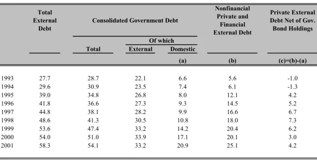
In summary, was Argentina’s foreign debt build-up process dominated by the public or the private sector? Table 4.5 shows that the economy’s total external debt increased from 27.7% to 58.3% of GDP between 1993 and 2001. About one-third of this change reflects higher public indebtedness, while the rest (2/3) seems to have resulted from aggressive private sector borrowing abroad. Indeed, private external debt increased from 5.6% of GDP to 25.5% during the period. One could view this as evidence that the private sector, rather than the public sector, was the primary culprit of the accumulation of net foreign liabilities.
However, at the same time the public sector was borrowing massively from the private sector in the domestic capital market (see table 4.5). Indeed, while the foreign public debt / GDP ratio showed little change after 1998, domestic public borrowing rose by over 10 percent points of GDP. This effectively means that the private sector was borrowing abroad on behalf of the government. As the government was putting pressure on domestic financial markets, the private sector was forced to resort to external markets to meet its financing needs.
Table 4.5 External Debt (Percentage of GDP)
Total External
Debt
Nonfinancial Private and
Financial External Debt
Private External Debt Net of Gov. Bond Holdings
Total External Domestic
(a) (b) (c)=(b)-(a)
1993 27.7 28.7 22.1 6.6 5.6 -1.0
1994 29.6 30.9 23.5 7.4 6.1 -1.3
1995 39.0 34.8 26.8 8.0 12.1 4.2
1996 41.8 36.6 27.3 9.3 14.5 5.2
1997 44.8 38.1 28.2 9.9 16.6 6.7
1998 48.6 41.3 30.5 10.8 18.0 7.3
1999 53.6 47.4 33.2 14.2 20.4 6.2
2000 54.0 51.0 33.9 17.1 20.1 3.0
2001 58.3 54.1 33.2 20.9 25.1 4.2
Consolidated Government Debt
V. THE BANKING SYSTEM:
LARGE VULNERABILITIES BEHIND A STRONG FAÇADE
A. Strengths
Hyperinflation and deposit confiscation at the end of the eighties31 wiped out
confidence in the peso and domestic financial intermediation. After Convertibility was enacted, a major effort was launched to recreate a solid financial sector mostly based in dollar-denominated deposits and loans. In 1995 Tequila contagion led to a run on 18% of total deposits and to systemic illiquidity which, in the absence of a domestic lender of last resort, required prompt support from the IFIs to avoid a collapse of the banking and payments systems. The authorities responded by “building” a large liquidity buffer and through other ambitious reforms in order to consolidate a highly resilient financial system. Results were impressive. By 1998 Argentina ranked second (after Singapore, tied with Hong Kong, and ahead of Chile) in terms of the quality of its regulatory
environment, according to the CAMELOT rating system developed by the World Bank 32
See Table 5.1 .
Table 5.1
Country Total Score*
Singapore 16
Argentina 21
Hong Kong 21
Chile 25
Brazil 30
Peru 35
Malasya 41
Colombia 44
Korea 45
Philippines 47
Thailand 52
Indonesia 52
Camelot Ratings for Banking System Regulation
*Lower numbers indicate better ranking
Source:World Bank. Argentina Financial Sector Review (1998)
31 The so-called Bonex plan instituted in 1989.