INSTITUTO TECNOLÓGICO Y DE ESTUDIOS SUPERIORES DE MONTERREY
PRESENTE.-Por medio de la presente hago constar que soy autor y titular de la obra denominada
, en los sucesivo LA OBRA, en virtud de lo cual autorizo a el Instituto Tecnológico y de Estudios Superiores de Monterrey (EL INSTITUTO) para que efectúe la divulgación, publicación, comunicación pública, distribución, distribución pública y reproducción, así como la digitalización de la misma, con fines académicos o propios al objeto de EL INSTITUTO, dentro del círculo de la comunidad del Tecnológico de Monterrey.
El Instituto se compromete a respetar en todo momento mi autoría y a otorgarme el crédito correspondiente en todas las actividades mencionadas anteriormente de la obra.
De la misma manera, manifiesto que el contenido académico, literario, la edición y en general cualquier parte de LA OBRA son de mi entera responsabilidad, por lo que deslindo a EL INSTITUTO por cualquier violación a los derechos de autor y/o propiedad intelectual y/o cualquier responsabilidad relacionada con la OBRA que cometa el suscrito frente a terceros.
Network-Induced Delay Models for Can-Based Networked
Control Systems Evaluation-Edición Única
Title Network-Induced Delay Models for Can-Based Networked
Control Systems Evaluation-Edición Única
Authors Rodrigo Vargas Rodríguez
Affiliation ITESM-Campus Monterrey
Issue Date 2007-12-01
Item type Tesis
Rights Open Access
Downloaded 19-Jan-2017 10:01:12
MONTERREY CAMPUS
GRADUATE PROGRAM IN MECHATRONICS AND INFORMATION TECHNOLOGIES
NETWORK-INDUCED DELAY MODELS FOR
CAN-BASED NETWORKED CONTROL SYSTEMS
EVALUATION
T H E S I S
PRESENTED AS A PARTIAL FULFILLMENT OF THE REQUIREMENTS FOR THE DEGREE OF
MASTER OF SCIENCE IN AUTOMATION
BY
Rodrigo Vargas Rodr´ıguez
BY
Rodrigo Vargas Rodr´ıguez
T h e s i s
Presented to the Graduate Program in Mechatronics and Information Technologies
This thesis is a partial requirement for the degree of Master of Science in
Automation
INSTITUTO TECNOL ´OGICO Y DE ESTUDIOS SUPERIORES DE MONTERREY
Division of Mechatronics and Information Technologies
Graduate Program in Mechatronics and Information Technologies
The members of the thesis committee hereby approve the thesis of Rodrigo Vargas Rodr´ıguez, Eng. as a partial fulfillment of the requirements for the degree of Master of Science in
Automation.
Thesis Committee
Rub´en Morales Men´endez, Ph.D.
Thesis advisor
Ricardo A. Ram´ırez Mendoza, Ph.D.
Synodal
Artemio A. Aguilar Couti˜no, Eng.
Synodal
Graciano Dieck Assad, Ph.D.
Director of the Graduate Programs in Mechatronics and Information Technologies
Abstract
Networked Control Systems (NCS) are a variation of traditional Point-to-Point control systems. In NCS, sensors and actuators may be physically distributed and a serial common-bus communication network is used to exchange system information and control signals. Because all components use the same communication network, network-induced delays make the system stochastic and hard to predict. The Quality of Control (QoC) of each closed-loop system in a NCS is strongly affected by the network-induced delay produced by sensors and control signals.
Controller Area Network (CAN) is a popular real-time field-bus used for small-scale distributed environments such as automobiles, and recently in aircraft and aerospace electronics, medical equipment, and factory and building automation. In CAN, the time delay exhibits a stochastic behavior and varies according to the network load. Since QoC is affected by delays, designing and evaluating a controller must take into account the effect of network-induced delays.
This thesis illustrates two models that play the role of classifiers and estimators for network-induced delays. Based on experimental delay measurements, the models can estimate the network load and predict future time delay values. The models were built following a statistical approach using a continuous Hidden Markov Model, and a histrogram-based approach. They were trained/tested using experimental data taken from a realCAN system with excellent results. The CAN system used to perform the experiments is a multiplexedCAN scale model from EXXOTestR, which is a training
unit with real components of a Peugeot 807.
In addition, two examples of the applicability of the models are illustrated. A
NCS simulator for evaluating systems under different network conditions, and a NCS
Dedicatory
To my father Rodrigo Vargas Esquivel
Patience is a virtue
To my mother Consuelo Rodr´ıguez Gamboa
Acknowledgements
To my advisor, Rub´en Morales Men´endez, Ph.D., for your support, commitment, and for the encouragement of making this thesis more than a graduation requirement. To Ricardo Ram´ırez, Ph.D., and Artemio Aguilar, Eng., for providing the necessary laboratory equipment, and for taking the time to meet and discuss the topics related to this work.
To Miguel de Jes´us Ram´ırez Cadena, MS, and Antonio Favela Contreras, Ph.D., for the given opportunity to be part of the Mechatronics Department at the Tecnol´ogico de Monterrey, campus Monterrey.
To Rosaura Arias, for your patience and love.
To my brothers Erick Vargas and Ronny Vargas, for your help, tips, and advices. To my friends at the Mechatronics Department: Celina Rea, Ariel Cano, ´Angel Orozco, Jorge Claros, Geovanna Ruffo, Ignacio Barradas, Juan Carlos Tud´on, Joel Castillo, Jorge Jim´enez, Aldo Cedillo, Jos´e Ernesto P´erez, Aline Drivett, Myriam Gonz´alez, Pedro Ju´arez, and all MATs I had the pleasure to meet and share with.
To Pablo Ordo˜nez, Pedro Carstensen, Julio ´Avila, Luis Carlos F´elix, and Jorge Gamboa, for always making great moments out of simple ones.
To all the members of the Mechatronics Department, specially to Amparo Herrera, Luis Rosas, Jos´e de Jes´us Rodr´ıguez, and Luis Garza.
To Juan Pineda, for your continuous support, advices, and for sharing your knowledge. Experience is always the best school.
To Pablo Mej´ıas, Carlos L´opez, Allan Rojas, and Camilo P´erez, for always leaving stress out of the equation.
To Ana V. Vargas Esquivel, for your support and prayers.
1 Introduction 1
1.1 Motivation . . . 2
1.2 Thesis . . . 2
1.3 Methodology . . . 2
1.4 Related Work . . . 3
1.4.1 Delay Modeling . . . 3
1.4.2 NCS Control Design . . . 4
1.5 Contributions . . . 4
1.6 Outline of the Thesis and Publications . . . 5
2 Problem Formulation 7 2.1 Time Delays in NCS . . . 7
2.2 Related Work . . . 9
2.2.1 Delay Modeling . . . 9
2.2.2 NCS Controller Design . . . 12
3 Controller Area Network 15 3.1 Controller Area Network . . . 15
3.1.1 Main Characteristics of CAN . . . 15
3.1.2 CAN and theOSI Model . . . 16
3.1.3 Physical Layer . . . 17
3.1.4 Data Link layer . . . 19
3.2 Summary . . . 21
4 Modeling of NCS 23 4.1 State Space Modeling . . . 23
4.2 State Space Representation for Systems with Delays . . . 24
4.2.1 Delay less than one sampling period . . . 24
4.2.2 Delay longer than one sampling period . . . 25
4.3 Summary . . . 26
5 Experimental Measurements 27 5.1 Experimental Platform . . . 27
5.1.2 Software Setup . . . 28
5.2 Design of Experiments . . . 29
5.3 Timing Analysis . . . 29
5.4 Summary . . . 31
6 Modeling Network-Induced Delays 35 6.1 Hidden Markov Models (HMM) . . . 35
6.1.1 Architecture of a HMM . . . 36
6.1.2 Delay Modeling Using HMM . . . 37
6.2 Histogram Parameterization (HP) . . . 38
6.2.1 Delay Modeling Using HP . . . 39
6.3 Summary . . . 41
7 Applications 47 7.1 Example #1: Control Performance Evaluation . . . 47
7.1.1 NCS simulator . . . 47
7.2 Example #2: Controller Design . . . 51
7.2.1 Control Law . . . 51
7.2.2 Estimator . . . 51
7.2.3 Results . . . 53
7.3 Summary . . . 54
8 Conclusions 61 8.1 Factors that affect network time delays . . . 61
8.1.1 Network Load . . . 61
8.1.2 Network Schedule . . . 62
8.1.3 Network Bandwidth . . . 62
8.1.4 Size of Messages . . . 63
8.1.5 Message Priority . . . 63
8.2 Time Delay Models . . . 63
8.3 Contributions . . . 64
8.4 Future Work . . . 64
Bibliography 67 A Experimental Setup 69 A.1 Node Connection and Communication . . . 70
A.2 Software . . . 72
A.3 Experimental Time Delay Measurements . . . 73
A.3.1 Clock Synchronization . . . 73
B Hidden Markov Model Algorithms 75
B.1 Forward-Backward Algorithm . . . 75
B.2 Viterbi Algorithm . . . 77
B.3 Baum-Welch Algorithm . . . 78
B.4 Software Tools . . . 80
C Additional Results 81 C.1 HMM Additional Results . . . 81
C.2 HP Additional Results . . . 86
1.1 Typical setup and information flow of a NCS . . . 1
2.1 Time delays in NCS . . . 8
2.2 Timing of signals in aNCS . . . 9
3.1 CAN protocol OSI/ISO layers . . . 18
3.2 CAN wiring diagram . . . 19
3.3 Dominant and Recessive states . . . 19
3.4 Example of bit-wise arbitration . . . 20
4.1 Packet arrivals in a NCS when delays are less than one sampling period 25 4.2 Packet arrivals in a NCS when delays are longer than one sampling period 26 5.1 EXXOTestR scale model . . . 28
5.2 Design of Experiments . . . 30
5.3 Delay measurements for 5 msperiodicity . . . 31
5.4 Histograms for low network load and 5 msperiodicity . . . 32
5.5 Delay measurements for different periodicities and low network load . . 32
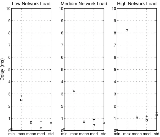
5.6 Boxplot for different periodicities and network loads . . . 33
6.1 Continuous HMM . . . 38
6.2 Modeling procedure . . . 39
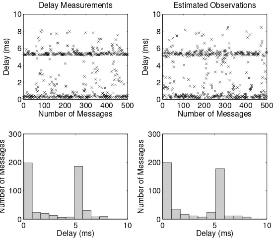
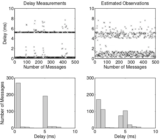
6.3 HMM low network load model performance - 5 msperiodicity . . . 40
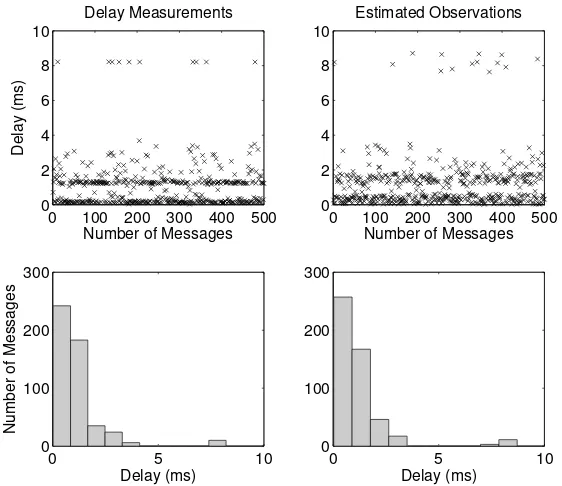
6.4 HMM medium network load model performance - 5 ms periodicity . . 41
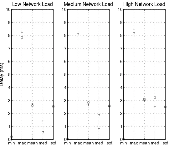
6.5 HMM high network load model performance - 5 ms periodicity . . . . 42
6.6 HP general model . . . 43
6.7 HP models performance for different parameters values. . . 44
6.8 HP low network load model performance - 5ms periodicity . . . 45
6.9 HP medium network load model performance - 5 msperiodicity . . . . 45
6.10 HP high network load model performance - 5 msperiodicity . . . 46
7.1 Application example #1 - Low Network Load . . . 48
7.2 Application example #1 - Medium Network Load . . . 49
7.3 Application example #1 - High Network Load . . . 50
7.4 Observer-based NCS controller using network-induced delay estimator . 52 7.5 NCS nodes execution flow chart . . . 55
7.6 NCS controller with low network load time delay estimator . . . 56
7.7 NCS controller with medium network load time delay estimator . . . . 57
7.8 NCS controller with high network load time delay estimator . . . 58
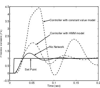
7.9 Constant-value vs HMM time delay models . . . 59
8.1 The constitution of network load . . . 62
A.1 A multiplexed CAN X3 scale model . . . 69
A.2 Nodes connection to the CAN system . . . 71
A.3 Load network application . . . 72
A.4 EXXOTestR USB-MUX-4C2L module . . . 73
C.1 HMM model performance - 1 msperiodicity and low network load . . . 81
C.2 HMM model performance - 1 msperiodicity and medium network load 82 C.3 HMM model performance - 1 msperiodicity and high network load . . 82
C.4 HMM model statistical analysis - 1 msperiodicity . . . 83
C.5 HMM model performance - 10 msperiodicity and low network load . . 83
C.6 HMM model performance - 10 msperiodicity and medium network load 84 C.7 HMM model performance - 10 msperiodicity and high network load . 84 C.8 HMM model statistical analysis - 10ms periodicity . . . 85
C.9 HP model performance - 1 ms periodicity and low network load . . . . 86
C.10 HP model performance - 1 ms periodicity and medium network load . 87 C.11 HP model performance - 1 ms periodicity and high network load . . . 87
C.12 HP model statistical analysis - 1 ms periodicity . . . 88
C.13 HP model performance - 10 ms periodicity and low network load . . . 88
C.14 HP model performance - 10 ms periodicity and medium network load . 89 C.15 HP model performance - 10 ms periodicity and high network load . . . 89
2.1 Related work summary in control networks time delay modeling . . . . 12
2.2 Previous work summary in NCS controller design . . . 14
3.1 ISO/OSI model . . . 17
6.1 Physical meaning of HMM parameters . . . 37
7.1 NCS observer-based controller performance . . . 54
A.1 Experimental setup devices . . . 70
Symbol Description
Continuous and Discrete Systems
k Sampling instant of a discrete system (integer value)
T Sampling period of a discrete system (in time units, e.g. mil-liseconds)
t Time in a continuous system
y(k) Process output at sampling instantk for a discrete system.
u(k) Control signal at sampling instantk for a discrete system
y(t) Process output at timet for a continuous system
u(t) Control signal at time t for a continuous system Time Delay
τ Time delay, the time it takes a message to be transmitted from the source node to the destination node
τsc
k Sensor-to-controller time delay at sampling instantk
τca
k Controller-to-actuator time delay at sampling instantk
τc
k Computation time delay at sampling instant k
τk Control time delay, it is defined as τk = τksc + τkc +τkca and
represents the time transcurred since a measurement signal is sampled at sampling instant k until it is used in the actuator
pk Predicted time delay value at sampling instantk
State Space
x State vector (n-vector)
u Control vector (r-vector)
y Ouput vector (m-vector)
A State matrix (n×n matrix)
B Input matrix (n×r matrix)
C Output matrix (m×n matrix)
D Direct transmission (or feedforward) matrix (m×r matrix)
t+
Continuous section of time
Kr Controller input gain matrix
Symbol Description
r Process reference signal Markov Theory
X State of a Markov process
§i State of a Markov process at time i N Number of states in a HMM
M Number of observation probability distributions in a HMM A HMM state transition probability distribution matrix
B HMM observation symbols probability distribution matrix
Introduction
Traditional control systems use a point-to-point architecture where each sensor and ac-tuator is connected through a single wire to the central control unit. This architecture has been implemented successfully in industry for decades. However, expanding phys-ical setups and functionality are pushing the limits of the point-to-point architecture.
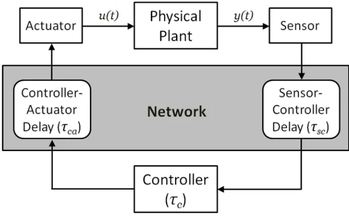
Networked Control Systems (NCS) are one type of distributed control sys-tems where serial communication networks are used to exchange system information and control signals (see Fig. 1.1). Common-bus based architectures offer several ad-vantages over the traditional point-to-point architecture: modularity, more efficient reconfigurability, decentralization of control, integrated diagnostics, better resource utilization, quick and easy maintenance, and low installation and maintenance costs [Dias Santos 03, Huo et al. 04]. The primary advantages ofNCS are modular and flex-ible system design, simple and fast implementation, reduced system wiring and ease of diagnosis and maintenance [Dias Santos 03].
Figure 1.1: Typical setup and information flow of aNCS. The communi-cation medium is shared by several users (controllers, actuators, sensors).
The communication networks used to support NCS are often called fieldbuses, or
control networks. A fieldbus is an industrial network system for real-time distributed control. There are a wide variety of fieldbus standards that can be used to implement a NCS, for example PROFIBUS in process control, CAN in automotive applications, and MODBUS for connecting industrial electronic devices.
Controller Area Network (CAN) is considered suitable to support small-scale NCS, due to their real-time capabilities [Huo et al. 04]. CAN is a serial communication protocol for distributed real-time control and automation systems. Although originally designed for automotive applications, the CAN protocol has many applications in other fields because of its simplicity and low cost.
1.1
Motivation
In NCS several issues arise due to data sharing a common network medium. The network itself is a dynamic system that exhibits characteristics which traditionally have not been taken into consideration in classical control systems design. These features relate specifically to the communication channel used, such as bandwidth and transmission errors [Quevedo et al. 04]. As a consequence, a network controller cannot be designed using standard algorithms and classical control theory.
When sensors, actuators and controllers exchange data across the network, vari-ous delays with variable length occur due to sharing the common network medium. These delays are called network-induced delays. Network transmission delays can vary widely according to the transmission time of messages and the overhead of the network. Usually, this network delay is randomly time varying.
Network-induced delays are inevitable and are the major cause of the deterioration of system dynamic performance and potential system instability [Li et al. 04]. There-fore, a major problem in the analysis and design of NCS is related to its stabilization using linear feedback. This demands a modeling approach for the network-induced delay.
1.2
Thesis
A network dynamic model based on statistical and/or probabilistic approaches allows the analysis and understanding of the effect of network-induced delays on the perfor-mance and stability of Networked Control Systems, specifically of a Controller Area Network.
1.3
Methodology
An experimental platform was setup in order to gather experimental network-induced delays. The setup consists of a CAN system with several nodes connected to it. In addition, a sender node and a receiver node were created, connected and synchronized in order to calculate transmission delays.
The CAN system used to perform the experiments is a multiplexed CAN X3 ped-agogic scale model from EXXOTestR, see Appendix A for details. The scale model is
a training unit with real components of the Peugeot 807 that integrates three differ-ent network types: CAN, LIN (Local Interconnect Network) and VAN (Vehicle Area Network).
In addition the EXXOTestR CAN system, a communications framework was
de-veloped in order to send the gathered data in the experimental platform to a computer for further processing.
A set of experiments were designed covering a wide range of network configurations, specially realistic scenarios found in real implementations of CAN systems. They were performed in the experimental platform, and experimental time delay measurements were stored and then statistically analyzed. Statistic profiles were obtained for each network configuration.
Once statistical profiles were obtained, statistical and probabilistic tools and tech-niques were used to model the network-induced delay. The models were then used to obtain delay observations for which statistical profiles were constructed and compared against the real network-induced delays profiles. A statistical analysis was performed to evaluate the developed models.
Finally, a NCS simulation tool was developed to test the applicability of the network-induced delay models in the design of controllers for systems with delays. The performance of the models were evaluated in terms of stability and performance in the simulated control-loop system. Again, a statistic analysis was performed to validate the applicability of the models.
1.4
Related Work
Recently most NCS research has focused on control techniques that deal with the uncertainty that network-induced delays introduce in control systems. Following is a brief description of previous work on delay modeling and control design for NCS.
1.4.1
Delay Modeling
The simplest model [Nilsson 98] consists of a Constant value model, and it has been used for applications where the delay introduced by the network is less than the applica-tion’s delay. [Nilsson 98] also uses a Random value model where the delay observation is taken from only one probability distribution.
Finally, [Feng-Li 01a, Feng-Li 01c] used histograms with different probability dis-tributions to model the network-induced delay.
Delay models are used to design and evaluate NCS controllers in terms of stability and performance. A model that exactly characterize the network-induced delay is difficult to obtain, but generally a good and reliable model has been used.
1.4.2
NCS
Control Design
Controller design forNCS has usually considered delays less than one sampling period. Because of this robust or optimal stochastic approaches have usually been chosen to deal with uncertainties in the system coming from transmission delays. [Huo et al. 04] and [Li 05] summarizes some of the robust and stochastic approaches that have been implemented.
Design for longer delays have also be studied, but they are restricted to a limited characterization of delay behavior, usually modeled as a constant value. [Chen 04] uses a state observer to reconstruct plant state at the time the control signal is calculated. And [Wang 03] presents an estimator that is used to predict plant state in order to calculate the appropriate control signal.
1.5
Contributions
A stochastic characterization of the network-induced delays for a real CAN system implementation is made. Different network configurations are analyzed and the factors involved in the degradation of stability and performance of control loops closed over a communication network are studied.
To guarantee the stability and performance of NCS, different network-induced delay models that can be used to design and analyze controllers were created. These models were then verified by simulation, experimental, and statistical analysis.
The design and analysis of a NCS controller is not the main contribution of this thesis, but the time delay models that support the design and evaluation process are. The main contributions of this thesis are summarized as follows:
• Characterization of network-induced delays in CAN-based systems.
• Based on network-induced delays and network characterization, network-induced delay models are created using different statistical and probabilistic techniques.
• The created stochastic models are then incorporated in control design method-ologies to design a controller for aCAN-based NCS.
1.6
Outline of the Thesis and Publications
The outline of the thesis is as follows:
Chapter 2: Problem Formulation
This chapter gives an introduction to the problem formulation. A short review of NCS
and how time delays affect control loops is presented. The chapter is concluded with a summary of work related to this thesis.
Chapter 3: Controller Area Network
In this chapter the CAN protocol is described, paying special attention in those char-acteristics that affect network transmission time delays.
Chapter 4: Networked Control Systems Modeling
A description of how time delays are included in the state representation of NCS is included in this chapter. Systems with time delays less than one sampling period and longer than one sampling period are studied.
Chapter 5: Experimental Delay Measurements
This chapter describes how experimental delay observations were registered and a tim-ing analysis for the CAN system is presented.
Chapter 6: Modeling Network-Induced Delays
Two models for the network-induced delays are developed based on statistical and probabilistic approaches. Both models are studied and evaluated. Results are shown comparing both models with the real delay observations and using statistical metrics.
Chapter 7: Applications
Applications for the network-induced delay models are described. Additionally an observer-based controller for NCS is developed based on the developed models. The controller is used as an example of how the models can be used. Results are shown for different network conditions and validated through statistical analysis.
Chapter 8: Conclusions
Appendices
The thesis is concluded with four appendices. Appendix A details the experimental setup, Appendix B describes HMM theory, Appendix C shows additional results, and finally Appendix D includes the international publications resulting from this work. International Publications
Vargas-Rodriguez, R. and Morales-Menendez, R., Network-induced Delay Model Using HMM for CAN-Based Networked Control Systems Evaluation. 6th EUROSIM
Congress on Modelling and Simulation, Ljubljana, Slovenia, September 2007.
Vargas-Rodriguez, R. and Morales-Menendez, R., Network-Induced Delay Mod-els for CAN-Based Networked Control Systems. 7th IFAC Int. Conf. on Fieldbuses
Problem Formulation
The change of the communication architecture from point-to-point to common-bus in-troduces different forms of stochastic time delay between sensors, actuators, and con-trollers. These time delays come from the time sharing of the communication medium as well as additional functionality required for physical signal coding and communica-tion processing [Feng-Li et al. 02].
The time delays introduced by the network medium are called network-induced delays. The network-induced delay leads to competition between the different system components because of the limited network resource (or finite bandwidth constraint). Only one node can access the network at a time.
Another important source of time delay, besides communication delays, is the computation-time delay of the controller (microprocessor or controller computer). The computation time is the time taken to execute programs that implement control algo-rithms at controller nodes or process data coding at sensor/actuator nodes.
The characteristics of the network-induced delays could be constant, bounded, or even random, depending on the network protocols adopted and the chosen hardware. In CAN, the bus access time is generally non-deterministic, meaning that network-induced delays are random and time-varying [Nilsson 98]. This type of time delay is the major cause of signal delay and distortion [Huo et al. 04]. They are inevitable and may cause system performance degradation and reduce the stability of the system.
2.1
Time Delays in
NCS
The two most important time delays that should be considered in control systems analysis and design are the end-to-end delays from sensor-to-controller, and controller-to-actuator.
There are essentially three kinds of time delays inNCS (Fig. 2.1):
• Communication time delay between the sensor and the controller τsc. • Computational time delay in the controller τc
• Communication time delay between the controller and the actuator τca.
Figure 2.1: Time delays in NCS.τsc is the sensor to controller delay, τca
is the controller to actuator delay, and τc is the controller computational
delay.
The control time delay τk for aNCS is the elapsed time since a measurement signal
is sampled at sampling instant k until it is used in the actuator. This delay is defined as τk =τksc+τ
c k +τ
ca k .
The time delays are an important problem in distributed control systems. They make the system varying, and theoretical results for analysis and design of time-invariant systems cannot be used directly.
From a sampled-data control perspective it is natural to sample the process output equidistantly with a sample period of h. It is also natural to keep the control time delay as short as possible. The reason is that time delays give rise to phase lag, which often degenerate system stability and performance.
The suggestion is to use an event-driven controller node and an event-driven ac-tuator node, while keeping the sensor node a time-driven node. This means that calculation of control signals takes place as soon as the new information arrives from the sensor node at the controller node. The timing in such a system is illustrated in Fig. 2.2. A drawback with this setup is that the system becomes time-varying. This is seen in Fig. 2.2 in that the process input is changed at irregular times.
Research inNCS has focused on two areas: communication protocols and controller design. A proper message transmission protocol is necessary to guarantee the network quality of service (QoS), whereas advanced controller design is desirable to guarantee the control quality of performance (QoP).
Figure 2.2: Timing of signals in a NCS. k is the sampling instant, h
is the time unit of the sampling interval, yk is the process output, uk is
the control signal, τsc
k is the sensor-to-controller time delay, and τkca is
the controller-to-actuator time delay. The first plot illustrates the process output at the sampling time, the second plot illustrates the signal into the controller node, the third plot illustrates the signal into de actuator node, and finally the last plot illustrates the process input.
applied directly when designing a CAN-based NCS. For this reason, a model of this phenomenon is needed in order to consider it during the design of the NCS.
2.2
Related Work
2.2.1
Delay Modeling
Most NCS modeling research has focused on state space representations that include the time delay features. Little attention has been paid to the characterization and modeling of the network-induced delays in order to obtain an evaluation framework based on a reliable model.
A comparison between three popular control networks is shown by [Feng-Li 01a, Feng-Li 01c]. Ethernet, ControlNet and DeviceNet networks are analyzed. The latter is based on the standard CAN specification. For each network type a detailed discussion of the medium access control (MAC) mechanism is provided. TheMAC is responsible for managing how nodes get access to the communication channel.
• Preprocessing time at source nodes
• Waiting time at source nodes
• Transmission time on network channel
• Postprocessing time at destination nodes
Because it is very difficult to identify each individual timing component [Feng-Li 01a] states that by monitoring time-stamped traffic the characteristics of each time delay component can be determined. An experimental study for nine identical devices on a DeviceNet CAN-based network was conducted.
Different time delay models were built based on statistic approaches. DeviceNet models were obtained based on histogram parameterization. The developed models can adopt four different configurations: zero, mean, normal and uniform. The zero
processing model lets the processing time equals zero; themean model uses the mean value as the processing time; the normal model assumes a normal distribution of the processing time; and theuniform model uniformly assigns the processing time for each message.
Finally, NCS design considerations and network performance and stability metrics are discussed and validated through theoretical and experimental analysis. The re-search shows the tradeoff between sampling time and network load and the acceptable working range of sampling periods in a NCS.
[Nilsson 98] identified that time delays in network transfer times vary due to varying network load, scheduling policies in the network nodes, and due to network failures.
Three models for network-induced delays are presented. The first is the simplest model, the time delay is constant for all transfers in the network. This model can be useful even if the system has varying delays, as in the case where the time scale (sampling time) in the system is larger than the delay introduced by the network. For this model the mean value or the worst case time delay value is used.
The second model treats delays as random and independent from each other. This assumption is made because the following system activities are not synchronized with each other and occur randomly:
• Waiting time for the network to become idle.
• Waiting time in queue, if other messages are waiting to be sent.
• Retransmission of messages because of transmission errors.
• MAC collision resolution may include a random wait to avoid collision at the next try.
network load, which vary with a slower time constant than the sampling period in the control system.
A different probability distribution can be used to represent the different types of time delays: sensor-to-controller τsc and controller-to-actuator τca.
The third model tries to model network components and phenomena such as queues and varying network load by including memory (state) using a Markov chain. With this model, different probability distributions can be used for τsc and τca, and each
probability distribution would belong to a certain network load.
Experimental measurements to create and analyze the models were gathered using a platform made of four computers equipped with CAN controllers connected to a
CAN system.
A methodology for modeling and analyzing NCS using HMM is presented by [Fu-Chun 05]. For this model the assumption that the network-induced delay is bounded and less than one sampling period is made.
Time delays are governed by an underlying Markov chain with unknown probability distributions. The observations of the Markov chain represent the time delay τk, which
is obtained by adding together τk =τsc+τca.
The HMM is used to represent the network load. That is, the observations of the
HMM represent the network load for the stochastic process being modeled. Three network loads were considered: low, medium and high.
The model is validated by developing an optimal state feedback controller and integrating the time delay model into a numerical simulation.
[Wei et al. 02] presented a model for network protocols and application performance evaluation. The model is a continuous-time HMM and it was built based on a series of end-to-end time delays and packet loss observations from an internet application. Packet losses were treated as very large delays in order to consider them in the model. To create the model, time delay values were discretized into a finite set of values. The set of discretized values constituted the set of observation symbols for the HMM. To obtain the set of observation symbols, the range of time delay values were divided into M equal length bins. A delay falling in the ith (1≤i≤M) bin is represented by
symbol i.
More formally, having an observation sequence{dt}T
t=1 the minimum and maximum
time delay values are denoted as dmin and dmax, respectively. The symbol dt = ∞ is
used to denote the observation at t as a loss; and the symbol dt =u is used to denote
that the observation at t is missing. The interval [dmin, dmax] is divided into M bins.
The length of each bin is denoted as b. Then b = (dmax −dmin)/M. Finally the time
delay and loss observations are converted to a symbol sequence {yt}T
t=1 as follows:
yt=
M dt=∞
dt−dmin
b dmin ≤dt< dmax
u dt=u
(2.1)
integrated to perform network protocol and application simulations under different network settings, representing real network scenarios.
The model was experimentally validated using the Transmission Control Protocol (TCP) and a streaming video application.
Previous work made in the characterization of time delays in control networks is summarized in Table 2.1.
Table 2.1: Related work summary in control networks time delay mod-eling. Constant or random values are the simplest models but do not consider network dynamics. Markov chain and HMM models consider the network load and use different probability distributions or symbols to represent time delays.
Model Author Year Limitations
Constant [Nilsson 98] 1998 Only useful if application has a larger delay than the introduced by the net-work delay.
Random [Nilsson 98] 1998 The delay values are taken from only one probability distribution, which is not useful for modeling different net-work conditions.
Markov chain [Nilsson 98] 1998 It uses one probability distribution per network load. It is not useful when delays cannot be characterized by only one distribution.
Histogram parameteriza-tion
[Feng-Li 01a] [Feng-Li 01c]
2001 Normal and uniform distributions may be too simple to represent CAN delays. Continuous
HMM
[Wei et al. 02] 2002 It uses a continuous-time Markov chain to represent the underlying stochastic process. The HMM is discrete and its observations represent the delays using a discrete domain.
HMM [Fu-Chun 05] 2005 Delays are governed by a Markov chain. The HMM is used to model the network load, not the actual delay.
2.2.2
NCS Controller Design
A compensation scheme forNCS with time delays longer than one sampling interval is presented by [Wang 03]. The presented scheme uses an estimator and time-driven and event-driven actuators simultaneously to make sure the process gets control signals in every sampling interval.
The estimator uses a fixed (constant) time delay valuep, which is obtained by cal-culating the worst-case delay time. The estimated value corresponds to the controller-to-actuator delay, and it is then used by the controller to calculate a control signal appropriate for the future system state. This is because the control signal may take several sampling intervals to get to the actuator.
Process state is fed into the estimator to reconstruct an approximation to the un-delayed process state and make it available for the control calculation. Then the next 2p−1 states are estimated in order to calculate the control signal than will be sent to the actuator.
The compensation scheme was validated using simulation and a random number generator to obtain time delay values.
[Huo et al. 04] presents a revision of the state of the art inNCS. The author states that robust H2 and H∞ controllers can be used by treating delays as uncertainties
and if the system structure is known. If system stability and performance needs to be analyzed and guaranteed a linear matrix inequality (LMI) approach can be used.
Other covered strategies to compensate for randomly varying time delays are stochastic control approaches such as LQG optimal controllers. Stochastic approaches are preferred for modeling time delay, but if stability wants to be guaranteed under system uncertainty then a robust controller design could be adopted.
[Chen 04] present a control strategy based on a state observer. In a time-driven
NCS all states of the process could not be directly observed because sensor signals may get delayed. In such cases the observer is used for reconstructing the states by estimating the full state of the process using partial measurements.
The observer-based control strategy was validated using simulation, both in a sys-tem with time delays and other without time delays.
[Li 05] also summarizes some common controller design techniques for NCS. Stan-dard LQR, Fuzzy Logic, and Model Predictive Control (MPC) controllers are de-scribed. In addition, the author comments that a robust approach could be applied to deal with NCS uncertainties, such as variance of time delays. Furthermore, it is said that a robust or stochastic controller might be conservative if the uncertainty cannot be exactly characterized.
Table 2.2: Previous work summary inNCS controller design. Controllers for HMM can be based on an estimator, or designed following a robust or stochastic approach. The latter is often chosen because it makes it possible to represent time delays as uncertainties, which allows time delays to be represented as a constant value (the worst case).
Model Author Year Limitations
NCS State Observer
[Wang 03] 2003 For systems with delays longer than one sampling period. It uses a fixed (constant) time delay value which is the worst-case delay time. Useful but does not really characterize system de-lays, thus making the system unstable as network load increase.
Robust H2,
Robust H∞,
and LQG op-timal control
[Huo et al. 04] 2004 Delays are treated as system uncertain-ties. Delays are not characterized; how-ever, since a robust approach is used system stability can be analyzed and guaranteed to a certain degree of un-certainty (or maximum delay value). Fuzzy Logic
and Model Predictive Control (MPC)
Controller Area Network
In this chapter a general overview on the CAN protocol is presented and its general characteristics are studied. The physical implementation of the protocol and how the access to the bus is granted is also studied for a better understanding on how time delays are originated.
3.1
Controller Area Network
Controller Area Network (CAN) is a communication bus for message transaction in small-scale distributed environments. Although originally designed for automotive ap-plications by R. Bosch [Bosch 91], CAN has rapidly gathered a growing attention in fields such as aircraft and aerospace electronics, medical equipment, and factory and building automation.
CAN is broadcast bus with a multi-master architecture able to provide real-time and fault-tolerance features extremely useful for control and automation.
A CAN system sends messages using a serial bus network, with the individual nodes (processors) in the network linked together in a daisy chain. Every node in the system is equal to every other node. Any processor can send a message to any other processor, and if any processor fails, the other systems in the machine will continue to work properly and communicate with each other. Any node in the network that wants to transmit a message waits until the bus is free. Every message has an identifier, and every message is available to every other node in the network. The nodes select those messages that are relevant and ignore the rest.
3.1.1
Main Characteristics of
CAN
TheCAN protocol implements a priority-based bus, with aCarrier Sense Multiple Ac-cess with Collision Avoidance (CSMA/CA) Medium Access Control method (MAC). In this protocol, any station can access the bus when it becomes idle. However, con-trarily to Ethernet-like networks, the collision resolution is nondestructive in the sense that one of the messages being transmitted will succeed.
There are 4 types of frames that can be transferred in a CAN network. Two of them are used during the normal operation of the CAN network: the Data Frame, which is used to transfer data from one station to another and the Remote Frame, which is used to request data from a distant station. The other two frames are used to signal an abnormal state of the CAN network: the Error Frame signals the existence of an error state and the Overload Frame signals that a particular station is still not ready to transmit data.
Bus signals can take two different states: recessive bits (idle bus), and dominant bits (which always overwrite recessive bits). The collision resolution mechanism works as follows: when the bus becomes idle, every station with pending messages will start to transmit. During the transmission of the identifier field. if a station transmitting a recessive bit reads a dominant one, it means that there was a collision with at least one higher-priority message, and consequently this station aborts the message transmission. The highest-priority message being transmitted will proceed without perceiving any collision, and thus will be successfully transmitted. The highest priority message is the one with most leading dominant bits on the identifier field. Obviously, each message stream must be uniquely identified. The station that lost the arbitration phase will automatically retry the transmission of its message.
3.1.2
CAN
and the
OSI
Model
The Open Systems Interconnection (OSI) model is a standard reference model for how messages should be sent between any two points in a telecommunications network. Products following the OSI standards will communicate properly between them. ISO
published the standard 7498 to define the ISO/OSI model.
In the OSI model, data communications are organized into a hierarchy of seven different functions. Each function is a separated layer in the model. The top layer relates directly to the software application or hardware device that seeks to send mes-sages across a network, while the bottom layer refers to the actual bit traffic. TheOSI
model protocol stack is depicted in Table 3.1.
When an application seeks to communicate across the network, it processes the message through the seven layers of theOSI model one by one, starting at layer 7 and ending at layer 1. Then, the bit traffic is sent across the network to the application or device meant to receive the message. The application receiving the message processes the message in reverse, from layer 1 to layer 7.
This means that each layer provides services to the layer immediately above it, and it uses the services of the layer immediately below it, but each layer otherwise works independently of all the others. The function of each layer is hidden from and transparent to the function of every other layer, except for the layers immediately above and below (for example, layer 5 has no direct contact with layer 2). The essence of the OSI model is that a network can pass data between two applications or processes using means that are completely transparent to those applications.
Table 3.1: ISO/OSI model. A standard reference model for commu-nication networks. Each layer provides different services that should be implemented by applications that exchange information using communi-cation networks.
Layer Name Description
Layer 7 Application It defines communications partners, type of service, and security.
Layer 6 Presentation It converts data from one format to another.
Layer 5 Session It opens, coordinates, and ends conversations and ex-changes of data between two applications.
Layer 4 Transport It manages error checking and verifies that packets are delivered.
Layer 3 Network It routes and forwards data to the proper destination. Layer 2 Data Link It builds data packets and synchronizes network traffic. Layer 1 Physical It conveys the actual bit stream across the network. Manages the hardware and the mechanical process for sending and receiving data.
data across a network will have a corresponding element in layer 4 in the database utility that is to receive that data. Each layer has its own set of rules to govern interactions with corresponding layers, and these rules are called layer protocols.
Many communications systems, however, do not use all seven layers in the reference model, and that includes CAN systems. The CAN protocol only addresses two of the seven layers, excluding the actual bus wiring (Fig. 3.1). These layers are the physical layer and the data link layer, which provide functionality for transmission of simple messages to trigger events or to provide monitoring values from sensors. This leaves the implementation of features concerning higher-level layers (such as fail-safe behavior and low power modes) as proprietary options.
3.1.3
Physical Layer
The physical layer is responsible for the connection between the nodes in a network, and the actual transmission of electrical impulses across a copper wire, coax or fiber optic cable, or wireless signal. It defines how signals are transmitted and therefore deals with issues such as timing, encoding and synchronization of the bit stream to be transferred, and often the type of pin connectors and cables to use.
Bit signaling on the bus line can take two possible representations: recessive, which only appears on the bus when all the nodes send recessive bits; dominant, which needs to be sent only by one node to stand on the bus. This means that a dominant bit sent by one node can overwrite recessive bits sent by other nodes. This feature is used for bus arbitration and will be explained in the Data Link Layer section.
Figure 3.1: CAN protocol OSI/ISO layers. Only the Physical and Data Link layers are covered by the CAN specification. Implementation of higher-level layer features are left as proprietary options.
of wires. This provides very reliable signal transmission despite low signal levels and common mode errors. The two wires are named CAN H and CAN L and are termi-nated using 120-ohm resistors, Fig. 3.2. It is also typical to use twisted pair wires to reduce electromagnetic interference.
For the two-wire bus the recessive bus state occurs when the CAN L and CAN H
lines are at the same potential (CAN L = CAN H = 2.5V), and the dominant bus state occurs when there is a difference in potential (CAN L = 1.5V and CAN H = 3.5V), Fig. 3.3. The CAN bus remains in the recessive state when it is idle.
As it can be seen, CAN uses a bus topology, which is inexpensive. It allows easy node connection and it is less prone to network failures.
Each bit is transmitted using theNon-Return-to-Zero encoding scheme. This code displays a low spectral density thus allowing a good utilization of transmission medium bandwidth.
The standardCAN Physical Layer specification defines built-in fault tolerance fea-tures, that allows network operation in harsh conditions but with a reduced signal-to-noise ratio. Standardized fault tolerance is based on single-wire operation and it is able to ensure continuity of network operation in the presence of:
• one-wire breakage
Figure 3.2: CAN wiring diagram. Physical media is typically a differen-tially driven pair of wires (CAN H and CAN L) configured in a two-wire bus with termination resistors.
• two-wire short-circuit
The standard specifications do not provide any means to tolerate the simultaneous breakage of both wires in the bus line.
3.1.4
Data Link layer
The Data Link Layer builds data frames (or packets) to hold (encapsulate) the data to be transferred across the network. Each data frame is assigned a unique identifier, which is used to identify the frames, determine access to the bus, and to detect errors. The uniqueness of each frame avoids the need of using addressing information (such as the IP protocol) since it can be used to establish an unambiguous association between the object identifier and the meaning of the data it contains.
This layer also performs a function called Medium Access Control (MAC) to pre-vent conflicts on the network when two different nodes try to access the network at one time. This is called bus arbitration. CAN use Carrier-Sense Multi-Access with Collision Avoidance (CSMA/CA) as its MAC method. The CAN protocol calls this
Non-Destructive Bit Wise Arbitration. It is not centralized, and it grants node access to the bus based on priority.
The CSMA access control is random access method, which means that any node can access the bus as soon as it is idle. All nodes monitor the network and wait and idle state in order to start transmitting; bus access conflicts are resolved through the bitwise comparison of data frames identifiers.
The CAN protocol controls bus traffic by allowing high-priority messages access to the bus over lower-priority messages. Every message begins with the arbitration field, which identifies the message and determines its priority. Each node attaches this field to a message it seeks to transmit. Whenever a node transmits the arbitration field, it listens to the bus at the same time. If the node that is transmitting a recessive bit detects a dominant bit on the bus, it automatically stops transmitting and becomes a receiver of the dominant message. Once the more dominant message has been trans-mitted and the bus becomes idle, the less dominant nodes are able to try again, see Fig. 3.4 for an example. The result is that no bandwidth is wasted, there are methods that a designer can use to predict the longest possible delay before any message is delivered. Note that every node in the network will look at every message transmitted on the bus. Most of the time any given node will ignore most of the messages it sees.
3.2
Summary
CAN was conceived for small-scale applications, specially automotive applications. It implements only two layers of the OSI/ISO network reference model, leaving much of the functionality provided by higher layers as proprietary implementations. Because of this, other implementations based on the original CAN specification have emerged. The functionality added by manufacturers in these higher-layer implementations has made it possible for the CAN protocol to be implemented in other fields such as medical equipment, off-road vehicles, maritime electronics, public transportation, and building automation.
CANOpen andDeviceNet are two examples of industrial control network protocols that were built on top of the original CAN specification. Some of the functionality added by these implementations include addressing schemes and time-stamped mes-saging.
Modeling of
NCS
The state space representation of a system is a mathematical model of the physical system. It is a set of input, output and state variables related by first-order differential equations. State space can be used for time-invariant linear and nonlinear systems. To model time variant systems or systems subject to noise or other stochastic events it is needed to slightly modify the general state space model to include such variations.
A study of NCS modeling in state space is presented in this chapter for a better understanding of how delays are considered during controller design and evaluation. Systems with time delays less than one sampling period and time delays longer than one sampling period are studied since there is a significative difference.
4.1
State Space Modeling
Based on control theory a process model can be written as follows: ˙
x(t) = Ax(t) +Bu(t)
y(t) =Cx(t) +Du(t) (4.1) and a traditional controller is defined as:
u(kT) =Krr(kT)−Kx(kT) (4.2)
where A, B, C are the state matrix, input matrix and output matrix, respectively. K
is the state feedback gain matrix, and Kr is the input gain matrix. All matrices are of
compatible dimensions and the sampling period T is fixed and known.
The time variable t can be continuous (i.e. t ∈ R) or discrete (i.e. t ∈ Z). In the latter case the time variable is usually indicated as k.
The state space representation 4.1 is used for Linear Time Invariant (LTI) systems and is suitable only for deterministic systems.
Since NCS introduce a new dynamic phenomenon to the processes, some changes must be done in the way they are represented. It is needed to include the time delay into the process state space representation in order to be able to design and analyze performance and stability of controllers.
4.2
State Space Representation for Systems with
Delays
When time delays come into play a similar approach of that shown in equation 4.5 is followed to represent a process. In addition, the configuration is assumed to be with clock-driven sensors, event-driven controllers, and event-driven actuators.
The input u(t) is assumed to be sampled and fed to a zero-order hold so that all components ofu(t) are constant over the interval between any two consecutive sampling instants, or
u(t) =u(kT), f or kT ≤t < kT +T (4.3)
For time-invariant controllers, the sensor-to-controller delay and controller-to-actuator delay can be lumped together as τ =τsc+τca.
For a system with no time delay (τ = 0) the state of the plant can be represented as follows [Ogata 95]:
x((k+ 1)T) =eATx(kT) +
Z T
0
eATBu(kT)dT (4.4)
However, in order to adapt the model to a NCS the equation 4.4 must be adapted to include the network-induced delay.
4.2.1
Delay less than one sampling period
When the delay time less than one sampling period (τ < T) at most two control samples, u((k−1)T) and u(kT), need to be applied during the Tth sampling period,
Fig. 4.1.
The system equations can now be rewritten as [Chen 04]: ˙
x(t) =Ax(t) +Bu(t), t ǫ [kT +τk,(k+ 1)T +τk+1]
y(t) =Cx(t) +Du(t)
u(t+
) =Krr(t−τk)−Kx(t−τk), t ǫ [kT +τk, k = 0,1,2, ...] (4.5)
whereu(t+
) is piecewise continuous and changes value atkT+τk. The control network,
shared by other nodes, is only inserted between the sensor nodes and the controller. Now, the system with sampling period T and time delay τk can be obtained as
follows:
x((k+ 1)T) = Φx(kT) + Γ0(τk)u(kT) + Γ1(τk)u(kT −T)
Figure 4.1: Packet arrivals in a NCS when delays are less than one sampling period [Zhang 01].
where
Φ =eAT (4.7)
Γ0(τk) =
Z T−τk
0
eAsBds (4.8)
Γ1(τk) =
Z T
T−τk
eAsBds (4.9)
4.2.2
Delay longer than one sampling period
If the delay τ is longer than one sampling period T, then it can be separated into two parts [Li 05]:
τ = (d−1)T +τ′
, 0< τ′
≤T (4.10)
where d≥2 is an integer valued parameter.
The networked closed-loop system can be written also as equation 4.5, but equation 4.6 must be rewritten as follows [Li 05]:
x(kT +T) = Φx(kT) + Γ0(τ′)u(kT −dT +T) + Γ1(τ′)u(kT −dT)
where
Φ =eAT (4.12)
Γ0(τ′) =
Z T−τ′
0
eAsBds (4.13)
Γ1(τ′) =
Z T
T−τ′
eAsBds (4.14)
When delays are longer than one sampling period, control signal packets and sample packets can switch places in time (see Fig. 4.2) or even be overwritten be newer values. The behavior will depend on the communication protocol. In either case, if the control signal ui arrives after uj, and i < j, ui should be ignored by the actuator.
In the same way, the controller should not send a new control signal if process sample yi arrives after yj, and i < j, although the state estimate should be updated,
see point C in Fig. 4.2.
Figure 4.2: Packet arrivals in a NCS when delays are longer than one sampling period [Wang 03]. Data packets can switch places in time (an older value may arrive after a newer value), as in points B and C.
4.3
Summary
Experimental Measurements
Characterizing real-world signals in terms of signal-models is a problem of fundamental interest. When these signals come from a stochastic process, statistical models are useful because they try to characterize only the statistical properties of the signal [Rabiner 89].
Typically, delays are modeled as a constant value or as a random value following a probability distribution for simplicity. More advanced techniques like Markov chains [Nilsson 98] and parameterization of histograms [Feng-Li 01a, Feng-Li 01c] have been used. However, these techniques sometimes fail to exactly characterize delays because of their restrictions in the number of probability distributions or because they use discrete domains to represent delays.
A good characterization of network-induced delays is important specially in those systems where good estimation is needed in order to assure system performance and stability. As it is known, good estimations depend on how good the estimator charac-terize the real world signal.
Following is a description of the experiments performed to gather experimental mea-surements and how they were characterized. Then a statistical analysis is presented, giving the required background for creating time delay models.
5.1
Experimental Platform
A full featured CAN system similar to the one used in a Peugeot 807 automobile was used as the platform for collecting time delay measurements.
Software tools were developed to vary the network load, to analyze time delay measurements, and to validate the models.
For a detailed description of the experimental setup see Appendix A.
5.1.1
Hardware Setup
The CAN system is a multiplexedCAN X3 pedagogic scale model from EXXOTestR,
shown in Fig. 5.1. The scale model is a training unit with real components of the Peu-geot 807 that integrates three different network types: CAN, LIN (Local Interconnect
Network) and VAN (Vehicle Area Network). The high speed CAN bus was chosen to perform the experiments.
Figure 5.1: EXXOTestR scale model. A network system from a Peugeot
807 automobile featuring low speed and high speed CAN buses. Two nodes were developed using FreescaleTM
Semiconductor microcontrollers. The nodes were used to send and receive timestamped messages over the network in or-der to calculate time delay values. A signal generator was used to synchronize the microcontrollers clocks and to establish the sampling interval.
Additionally, a communication channel was developed between the microcontrollers and a computer in order to send the gathered data in the experimental platform for further processing.
5.1.2
Software Setup
To load the network a software program was developed in LabWindowsTM
/CVI from National InstrumentsTM
. To interface the software with theCAN bus the EXXOTestR
USB-MUX-4C2L module and the MUXDLL dynamic link library, also provided by EXXOTestR, were used. The application was used to load the network with periodic
messages and monitor the network load status.
To analyze the gathered data, and to create and validate the models the software MATLABR from The Mathworks was used. AHidden Markov Model (HMM) Toolbox
5.2
Design of Experiments
A series of experiments were designed to determine network-induced delays in the transmission between two nodes connected to the CAN system. The experiments were divided in sets in order to measure time delays as a function of network load, periodicity and priority. All experiments used embedded timestamps in the messages, which were used to calculate the time delay. The time delay is obtained by subtracting the reception timestamp to the transmission timestamp.
Several factors can affect message time delays. Network load, the priority of the messages, data packet length, message scheduling and transmission periodicity are the most influential factors.
For all messages the data packet size was held constant at 8 bytes, which is the maximum size for the standard CAN message format. The scheduling was also held constant because the EXXOTestR scale model already has a predefined schedule based
on a real automobile implementation. Message priority was changed using one low priority and one high priority message id. Transmission periodicity was also changed, using 1 ms, 5 ms and 10 ms transmission periods. Finally, the network load was modified using different periodic messages.
Because of the network nodes that already exchange information when the automo-bile (EXXOTestR scale model) is turned on, the lowest network load was 14%. This
condition simulates a car under normal operation. Then periodic messages with low and high priorities were setup in order to load the network. Three network loads were implemented: low load (14%), medium load (38%) and high load (73%).
Experiments were constructed for 18 different network settings. Each setting con-stituted a total of 1,000 samples divided in 10 sets (runs) of 100 samples each one. Network settings were adjusted by making combinations of message’s priority, trans-mission periodicity and network load, Fig. 5.2. For each message, transtrans-mission and reception timestamps were recorded in the microcontrollers’ memory.
5.3
Timing Analysis
Time delays in NCS can be broken into three parts:
• Time delay at the source node, which includes the preprocessing timeτpre involved
in encoding the data in an appropriate network format and the waiting timeτwait
it takes for the message to be sent.
• Transmission time delayτtx. It is the propagation time; that is, the total time it
takes a data packet to be completely transmitted through the network.
• Time delay at the destination node τpost, which includes only the time it takes
the destination node to decode the data packet and make it available for use. Thus, the time delay can be explicitly expressed by:
Figure 5.2: Design of Experiments. Combinations of different values for the factorsmessage priority,periodicity of messages, and network load
were made to gather experimental time delay observations on different system conditions.
However, since it is very difficult to identify each individual timing component in practical applications, the time-stamped traffic is monitored and the time delay is computed as follows:
τ =Tdest−Tsrc (5.2)
where Tsrc is the time when the message was sent, and Tdest is the time when the
message arrived to the destination node.
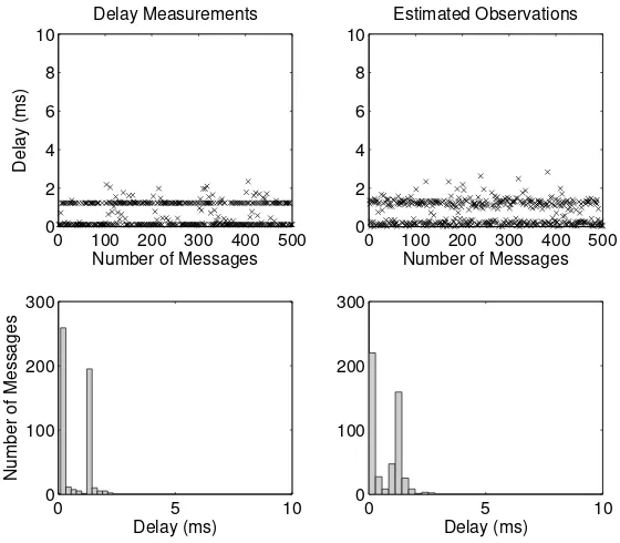
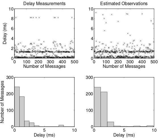
Fig. 5.3 shows time delay measurements for a network setting of 5msof periodicity, low message’s priority, and the three different network loads. Similar results were obtained for 1 ms and 10 ms. Since the behavior of the observed network-induced delay is similar for the different tested scenarios, only the 5ms periodicity results will be included in this section, for additional results refer to Appendix C.
As observed in Figures 5.3-5.4, delays tend to be near 0 ms and near 3 ms, such behavior was also noticeable in [Nilsson 98]. In addition, as the network load increase delays tend to disperse more, reaching peaks near 10 ms.
The same tendency can be observed for different periodicities, as shown in Fig. 5.5. The difference is that the upper bound for the maximum delay will vary according to the periodicity used for message transmission. This can be better seen in Fig. 5.6.
It is important to remark that the time delays shown in this chapter are one-way delays; that is, either sensor-to-controller or controller-to-actuator. This means that the control time delay τk can be significantly high (up to 8 sample times at 1 ms, as
0 100 200 300 400 500 600 700 800 900 1000 0
2 4 6 8
Messages for Low Network Load
0 100 200 300 400 500 600 700 800 900 1000 0
2 4 6 8
Messages for Medium Network Load
Delay (ms)
0 100 200 300 400 500 600 700 800 900 1000 0
2 4 6 8
Messages for High Network Load
Figure 5.3: Delay measurements for 5msperiodicity. Time delay values get higher and more disperse as the network load increase.
5.4
Summary
In order to analyze NCS it is important to study the characteristics of the network-induced delays and their impact on control applications. The timing analysis presented in this chapter serves as a foundation for identifying the network parameters and node configuration parameters that affect time delays.
Time delays in theCAN system used for this study are stochastic but statistically they behave in a certain way. This means that a simple constant or random-based model cannot be used to exactly characterize time delays.
0 2 4 6 8 0
100 200 300 400 500
600Low Network Load
Number of Messages
Delay (ms)
0 2 4 6 8
0 100 200 300 400 500
600Medium Network Load
Number of Messages 0 2 4 6 8
0 100 200 300 400 500
600High Network Load
Number of Messages
Figure 5.4: Histograms for low network load and 5 msperiodicity. The number of time delay values near zero decrease as the network load in-crease. Instead, time delays disperse more.
0 200 400 600 800 1000
0 1 2 3 4 5 6 7 8
Number of Messages
Delay (ms)
1ms 5ms 10ms 20ms
1 ms 5 ms 10 ms 0
1 2 3 4 5 6 7 8
Delay (ms)
Periodicity Low Network Load
1 ms 5 ms 10 ms 0
1 2 3 4 5 6 7 8
Delay (ms)
Periodicity Medium Network Load
1 ms 5 ms 10 ms 0
1 2 3 4 5 6 7 8
Delay (ms)
Periodicity High Network Load
Modeling Network-Induced Delays
In this chapter, two statistical and probabilistic approaches for modeling the network-induced delay are presented: Hidden Markov Model (HMM) and Histogram Parame-terization (HP).
Both models are used to characterize the statistical properties of a series of time delay measurements. Characterization means obtaining parameters for each model that can be used to represent the dynamics of the system being modeled. The ex-tracted parameters can then be used to perform further analysis and to simulate the system. HMM is generally used for pattern recognition and histograms are often used to characterize signals in terms of probability distributions and categories of data.
A statistical analysis was developed to evaluate the performance of the models. The five fundamental time delay statistics [Feng-Li 01b] were computed for the experimental measurements and the estimated observations: minimum, maximum, mean, median and standard deviation.
6.1
Hidden Markov Models (
HMM
)
A HMM is a doubly stochastic process with an underlying stochastic process that is
not observable, it is hidden. This hidden process can only be observed through another set of stochastic processes that produce the sequence of observed symbols.
In a HMM the system being modeled is the hidden process. It is assumed to be a Markov process with unknown parameters, and the challenge is to determine the hidden parameters from the observable variables.
In a regular Markov model the states are directly visible to the observer, and therefore the state transition probabilities are the only parameters. In a HMM the states are not directly visible, but variables influenced by the states are visible. Each state has a probability distribution over the possible output tokens. Therefore the sequence of tokens generated by an HMM gives some information about the sequence of states.
A random process is a Markov process X(t) if the future of the process given the present is independent of the past, that is, if for arbitrary times t1 < t2 < . . . < tk <