0
ISSN 1692-2611
Borradores Departamento de Economía
Medellín - Colombia
_______________________________________________________________________________________ La serie Borradores Departamento de Economía está conformada por documentos de carácter provisional en los que se presentan avances de proyectos y actividades de investigación, con miras a su publicación posterior en revistas o libros nacionales e internacionales. El contenido de los Borradores es responsabilidad de los autores y no compromete a la institución.
Click aquí para consultar todos los borradores en texto completo
N°39
Mayo de 2011
Per Capita GDP Convergence in South America, 1960-2007
Elaborado por:
Danny García Callejas
1 Per Capita GDP Convergence in South America, 1960-2007
Danny Garcia Callejas
- Introduction. – I. Convergence: From the Neoclassical Growth Model to Economic Geography. – II. Empirical Evidence of Convergence and Divergence in Latin America. – III. Testing Convergence in South America: Method and Results. – Conclusion and Policy Implications. – References.
Resumen:
Este artículo analiza la convergencia de la producción per cápita y los patrones de especialización en Sur América. Este estudio encuentra evidencia a favor de divergencia en la producción, sin embargo, también halla que diferencia en los patrones de especialización y producción no son, necesariamente, la causa. Por último y aunque más investigación es necesaria, este artículo sugiere que la integración regional y la geografía pueden tener un papel fundamental en explicar la convergencia de la producción.
Abstract:
This paper analyzes output per capita convergence in South America and production specialization patterns. This study finds evidence of output divergence; however, it also finds that structural output differences and patterns of specialization of production are not necessarily the cause. Finally, this paper suggests that geography and regional integration may play a pivotal role in explaining convergence of output, although more research is required.
Palabras clave: Club de convergencia, comercio, convergencia, geografía económica,
producción per cápita, Sur América.
Key words: Convergence, convergence club, Economic Geography, output per capita, South
America, specialization, trade.
Clasificación JEL: O47, F10, F43.
Professor, Economics Department, Universidad de Antioquia, Medellín, Colombia.
2
Introduction
Are South American countries converging? Since 1975, Latin America has followed a path of structural reforms in hopes of bringing sustainable and high growth back. Trade liberalization and financial reform became common in Argentina (1978), Chile (1975), Uruguay (1985), Bolivia (1986), Paraguay (1988), Venezuela (1989), Brazil (1990), Peru (1990) and Colombia (1990 and 1991). Although each reform was adapted to each
country’s economic structure, in general they all shared several common features like
reducing tariffs, reducing restrictions for capital mobility and promoting economic integration in the region.
Structural reforms in Latin America provided a more homogeneous institutional environment in the region. Moreover, they facilitated the integration of markets for products and, in some cases, for factors. This added up to some of the common cultural characteristics and historical background and idiosyncrasies in the region, led to believe that the underlying conditions of the neoclassical growth model might be fulfilled. Consequently, output convergence in South America might be a possibility.
The purpose of this paper is to revisit the debate of per capita GDP convergence among 10 South American countries during the period 1960-2007, using data from the World Development Indicators and some local South American Statistical Agencies. In doing so, this paper will use a stochastic convergence approach following Choi (2004). By analyzing the impact of shocks on per capita outputs, this research will try to establish whether economies converged for this period.
Outputs are influenced by a number of factors. Not only factors of production determine the level of production for a given year also weather conditions, geographic conditions and infrastructure, technology and available resources at the time of production, among others. Furthermore, when comparing two or several countries’ outputs—relative outputs—these features have crucial influence in determining the differences. Wars, internal conflicts, natural disasters, riots, civil unrest, financial crises, political turmoil or large price swings on export products are assumed as exogenous shocks that induce production to deviate from a steady path and increase differences in relative outputs among countries.
A country is said to follow a steady output path or pursue a steady state if it exhibits an output path consistent with a ―stable‖ production growth rate with few and mild
3 natural disasters, political turmoil at some point in their history, and their level of
productions are getting ―relatively‖ closer through time, then their outputs stochastically
converge.
This study will test if 10 South American countries have stationary relative outputs. The presence of a unit root at the first level of the variable would indicate that this set of countries do not have stationary relative output and thus do not converge. In order to test
for ―convergence clubs‖ or that subgroups of countries converge, the ten countries are
divided in four regions according to their historical relations and geographic proximity. The ten countries and there region are: Colombia, Ecuador and Venezuela, North region; Bolivia, Paraguay and Peru, East region; Brazil and Uruguay, West region; and Argentina and Chile, South region. The countries in the North region were one country until 1831—
The Great Colombia. In the East region, Bolivia, Peru and a part of Paraguay constituted one country until 1839—The Peruvian Bolivian Confederation. The west region was one
country until Uruguay’s independence in 1825. Finally, Chile and Argentina are grouped
due to geographic proximity and sharing the largest border with one another.
The evidence provided in this study suggests that there is no regional stochastic convergence for South American countries selected in this sample. The results also indicate that there are no convergence clubs or convergence as a whole. These results are in accordance with Dabus and Zinni (2005) that find divergence for a group of 23 Latin American countries for 1960-1998 and using a panel data technique. In the best of cases, these authors find conditional and absolute convergence at high implausible speeds when adding control variables; an indication of divergence in Latin America. Dobson y Ramlogan (2002) and Caceres and Nunez (1999) also find divergence using a time series and unit root approach.
Some of the possible explanations for divergence in South American countries are that these countries are not as integrated as required to foster convergence. However, some research argues that integration does not necessarily promote convergence (Walz, 1999). Another explanation is the existence of multiple equilibria and poverty traps (Quah, 1996; Durlauf and Johnson, 1995; Galor, 1996). Finally, it is possible that institutions and geography (Acemoglu et al., 2004) or technological diffusion via trade and foreign investment (Barro and Sala-i-Martin, 2004; Romer, 1990) is not promoting innovation or
imitation allowing countries to ―catch up‖ by technological or productivity
improvements.
4
I. Convergence: From the Neoclassical Growth Model to Economic Geography
A. The Basic Theory
1. Beta convergence
The neoclassical growth model developed by Solow (1956) and Ramsey (1928) suggests that economic production is a consequence of combining physical capital, human capital—in modern versions, labor and technology. However, the intensive use of these factors of production, specially capital, implies that each additional unit used in the production process provides a lesser return than the previous one. In other words, capital presents diminishing returns—as well as labor—implying that in the long run the only source of economic growth is labor force growth. If this rate of growth is constant, then economies achieve a situation in which output per worker and capital per worker do not change over time. This state is also known as a steady state.
The neoclassical growth model prediction of economies reaching a steady state in the long run implies that comparing two identical countries but on different stages in their path towards the steady will converge to the same level of output per capita and capital per capita in the long run. In other words, in the long run the poor country catches up with the rich country because the poor one grows faster than the wealthier one. This
―catching up‖ process is known as absolute convergence and it does require that both
countries converge to the same steady state.
Absolute convergence implies that there is a negative relation between initial income per capita and the growth rate of income per capita. These are the main factors included in any empirical verification of this hypothesis. The empirical equation—cross-country regression—to estimate for a group of economies, i = 1,.., n, follows.
T i i T
i it
u y T
e y
y
T 0 log(ˆ0) 0,
) 1
( log
1
(1)
Where T represents the total number of periods to analyze; yit is per capita income; yi0 is initial per capita income; α is a constant or intercept term; ŷi0 is the effective income per
capita level in the steady state, in other words, the long run income per capita excluding the growth rate of technology (in terms of effective labor); β is the speed of convergence; and uio,T is the error term. The left hand side of this equation is the average growth rate for this economy in the studied time period whereas the right hand represents the speed and time required in getting to a steady state situation.
5
log(yit) = a + (1 – b) • log(yit-1) + uit (2)
Assuming that i = 1, …, ζ, or the number of economies to compare; t = 1, …, T, or the
number of years available for the data; yit is the level of GDP per capita for country i in period t; and yi,t-1 is the one year lagged value of GDP per capita for country t. The coefficients to estimate are a and b. If there is absolute convergence then 0 < b < 1; and the higher the b, the greater the inclination towards convergence.
However, absolute convergence assumes that countries are identical or have very similar characteristics; this is a strong assumption, however. Thus, conditional convergence allows for convergence to occur and be compared among countries that have different economic structures but conditioned on controlling for those differences. If countries that have a higher growth rate also have a lower initial income when compared with others, after controlling or conditioning growth on the different characteristics—saving propensity, for example—and present evidence of closing the gap with respect to wealthier countries, then we describe this phenomenon as conditional convergence.
Barro and Sala-i-Martin (1991) propose estimating the following equation for conditional convergence: T i it i T i it u X y T e y y
T 0 log( ˆ0) 0,
) 1
( log
1
(3)
where Xit is a set of variables that control for the different steady states that countries in the sample might have. A common empirical version of the conditional convergence equation is as follows:
T i it it it i T i it u Pop I H y T e y y
T 0 log(ˆ0) 0,
) 1
( log
1
(4)
where the set of control variables are human capital (H), investment (I) and population
growth (Pop). In all cases, a 0 < β < 1 is evidence favoring convergence (similar to (2)).
2. Sigma Convergence
6 situations of high inequality of income or output. In order to include this feature, Quah (1992, p. 4) suggests analyzing variation of income per capita between and within countries. Sigma convergence ( -convergence) is the decline in the variation and dispersion of real income per capita within and between the countries being compared.
The empirical way of testing for -convergence is through the standard deviation of real per capita income throughout countries per each time period. The existence of -convergence or that countries are improving their distribution of income requires the existence of β-convergence. The opposite, however, is not true (Higgins et al., 2007). The reason is that a declining variation among and within countries— -convergence— implies that each countries mean income is getting closer and closer to the grand mean or mean of the incomes of all countries included in the sample. This is only possible, if
those countries with low average levels of income are ―catching up‖ to those with high
levels of income—β-convergence—; thus variation must be falling.
Sigma-convergence requires beta-convergence. Specifically, beta-convergence is necessary for the existence of sigma convergence. This implication can be analyzed as follows. Beta-convergence means that poor countries are growing faster than rich countries. Suppose that poor countries surpass rich countries in period T and that income per capita levels are now reversed, having rich countries the equivalent to the initial income that poor countries have and vice versa; and thus, maintaining the same distance in absolute terms. In this case, there is evidence for beta convergence since the poor caught up and even left the rich behind, in per capita terms. However, inequality still prevails since the rich are lagging in the same amount as the poor where in the beginning of this situation. Consequently, sigma convergence does not exist although beta convergence does.
Formally, Higgins et al. (2007) proves that beta convergence is a necessary but not sufficient condition for sigma convergence. Following Higgins et al. (2007), the empirical equation for β-convergence for a set of countries (i = 1, …, ζ) for a specific
period of time (t= 1, …, T) can be written as follows:
it it it
it y X u
y (1)log( )
log 1 (5)
Where β(0, 1); uit ~ (0, u2) and independent over t and i. Also, yit is the level of GDP
per capita for country i in period t; and yit-1 is the one year lagged value of GDP per capita for country t; and Xit is a set of control variables that could be human capital and investment, for example as in (4). After several manipulations Higgins et al. (2007, p. 6) show that:
t
tt c
2 2
2 0 2 2
2 1 1
7 Where c is a constant; ( 2)* is the steady state variance; 02 is the initial variance or
variance at t = 0 and β is the parameter for convergence. The consequence of this result is that if β(0, 1), then sigma convergence is possible since t2 would be stable. Finally,
Higgins et al. (2007, p. 7) also point out that in empirical studies sigma convergence
would also depend on ―whether or not disturbances are correlated, and have constant variances, across time and economies.‖
B. Some Empirical Studies
1. Beta convergence
Delong (1988) criticizes Baumol (1986) for obtaining convergence by using a sample that has selection bias. Including Norway but not Spain or Canada but not Argentina misleads the estimation. Furthermore, asking if countries have converged or not by picking those countries that today are rich but in 1870 were not is problematic. That ex-ante selection should cast doubt on the results. Finally, measurement error is also a problem since rich nations in 1870 that are also rich today but not as rich are more probable to have data available and old data tend to be more imprecise. Thus, measurement error is plausible and troublesome since we are analyzing those countries that we already know have
―converged.‖ Once measurement error and sample selection bias are corrected in Baumol
(1986), evidence of convergence disappears (Delong, 1988).
8 Table 1. Economic Growth and Convergence for World Data
Source Dependent
variable y0 h0 sk n Other Variables
Sample and Time
Landau (1983) gQ 0.0021 (6.18) (7.64) 0.026 GCONS( - ), POP(O), CLIM(Y) 1961-1976 96 countries
Landau (1986) gQ - 0.311 (4.80)
0.032 (4.87)
0.059
(1.37) - 0.262 (1.35)
POP(O), GCONS(-), GINV(O), GED(O), T(O), INF( - ), OIL(+), DP(-)
1960-1980 65 countries
Kormendi and
Meguire (1985) gY
-0.0063 (3.50) 0.57 (0.17) SDY(+), SRM(-), MDEXX(+),MDINF(-) 1950-77 47 countries 0.0086
(4.90) (3.30) 0.12 (0.15) 0.60
SDY(+), SRM(-), MDEXX(+), MDINF(O)
Baumol et al. (1989) gY
0.622 (1.72) 1.615 (5.00) 1960-1981. 103 countries. -1.47 (2.47) Grier and
Tullock (1989) gQ
-0.00083 (8.61)
Period dummies, SDY( + )
MDGC( - ), INF(O), MDINF(O), SDINF( - )
1951-80 24 OECD countries 0.00057 (1.89) Period dummies, SDY(+), MDGC(-), INF(-), MDINF(O), SDINF(-)
1961-80 89 ROW countries
Barro (1991) gQ
-0.0075 (6.25)
0.0305 (3.86)
0.064
(2.00) - 0.004 (3.07)
CCONS( - ), DISTOR( - ), REV( - ), ASSAS( - )
1960-1985 98 countries 0.025 (4.46) 0.00077 (8.56) 0.01 (1.15) Dowrick and
Nguyen (1989) gY * 100 (9.67) -2.01 (2.54) 0.064 (0.155) 0.58
Source: De La Fuente (1997, p. 48 and 49).
Note: The dependent variable is the average growth rate of real per capita income (go) or of aggregate real income (gr)
during the sample period. When the dependent variable is gr, the null hypothesis is that the coefficient of population
growth will be smaller than one, rather than negative as is the case when the dependent variable is gQ, t statistics (in
parentheses) or standard errors [in brackets] are shown below each coefficient.
Landau (1986) and Grier and Tullock (1989) use pooled data (with 4- and 5-year subintervals respectively); the rest of the regressions use cross-section data by countries.
( + ) and ( - ) indicate a significant coefficient of the corresponding sign; (Y) denotes significance, and (0) lack of it. Definition of ho: (*) = secondary enrollment rate, (**) = primary enrollment rate. Landau uses a weighted average of
three enrollment rates (primary, secondary, and university).
Other variables: GCONS = public consumption/GDP; POP = total population; CUM = climate zone dummy; T = trend; GINV = public investment/GDP, GED = public expenditure in education/GDP; INF = inflation rate; OIL = dummy for
oil producers; DP = distance to the closest harbour; DISTOR = Barre’s index of distortions affecting the price of capital
goods; REV = number of coups and revolutions; ASSAS = number of political assassinations; SDY = standard deviation of real output growth; SRM = standard deviation of money supply shocks, MDEXX = mean growth of exports as a proportion of output; MDINF average growth of inflation; MDGC = rate of growth of government’s share
9 Sala-i-Martin (1996) concludes that in general, when convergence is found, the average rate of convergence is 2%. This means that the approximate time required to close half of the gap—half-life—in income between high and low income world economies is 35 years.
For the case of Korea, Koo et al. (1998) find evidence of beta and sigma convergence in the 1967-1992 period. They estimate a speed of convergence of 4.5% or that the estimated half life to close the income gap among Korean regions is 15 years. However, their results are not consistent and present several structural breaks suggesting that the estimated coefficients are not constant for all sub-periods. Furthermore, the analysis suggests large swings among coefficient associated with convergence, casting doubt on this result. In general, it seems to be a rule that convergence speeds greater than 2% are suspicious.
Nevertheless, one possibility for irregular speeds of conversion is regions not being analyzed as groups; this points to the notion of convergence clubs (Baumol and Wolff, 1988). Convergence clubs are a set of economies that have share technology or received the positive spillovers of technological improvements from their ―club members‖
allowing them to increase international trade and investment. These elements combined with education, should encourage all members of the club to increase their productivity levels, thus promoting convergence. However, DeLong (1988) critizes this notion by implying that convergence clubs are a way to justify the existence of convergence among a set of countries and not others, indicating that those that are not members of the club should follow the same institutional arrangements as club members. One can infer, then,
that convergence clubs are ―forcing‖ convergence to show up in empirical estimations by
being a ground for justifying selection bias in the sample of club members.
Siriopoulos and Asteriou (1997) also challenge the notion of convergence clubs but empirically. These authors analyze the case of 13 regions in Greece for 1971-1996. The authors run regressions on absolute and conditional convergence for 3 periods: 1971-1981; 1981-1996; 1981-1996. In all cases the authors find no evidence of convergence among Greek regions. The authors also test for convergence clubs by separating the regions into the Northern and Southern region; however, their estimations also provide weak evidence in favor of conditional convergence. Yet, their results improved when dividing the data by groups of regions, no club convergence was found.
2. Sigma Convergence
Tsionas (2000) finds evidence of sigma divergence in the U.S., concluding that the dispersion of income has not declined over time. Similar results are obtained by Higgins et al. (2007) at the national and state levels but using a larger and longer data set for the U.S.
10 countries. Specifically, he finds that the variation among social expenditure within the Nordic (Denmark, Sweden, Finland Netherlands), Anglo-Saxon (Ireland and the UK), Conteninental (Austria, Belgium, France, Germany and Luxembourg) and Mediterranean (Greece, Italy, Spain and Portugal) regions have diminished over time but not between them. In other words, social expenditure keeps being unequal among these regions for the 1980-1999 period in Europe.
Lacas (2001) provides evidence on sigma-divergence in regions of Finland for the 1985-1995 period. However, he compares this case with the province of Quebec in Canada and finds that the opposite is true for this region. However, a stronger convergence is observed in the 1985-1990 subperiod.
Nevertheless, Rey and Dev (2004) caution on the bias created by spatial effects on sigma convergence estimations. Their study is pointing to the fact that geography matters (Krugman, 1991). In fact, regions tend to sigma-converge because there are similar structural and geographical characteristics that are not common with other regions or countries. Connectivity through integrated road systems, communication systems and research networks provide positive externalities enjoyed by the region but that as distance, for example, increases become costly to share.
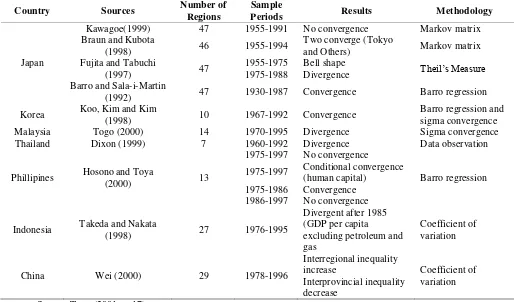
11 Table 2. Convergence Studies for Asia
Country Sources Number of
Regions
Sample
Periods Results Methodology
Japan
Kawagoe(1999) 47 1955-1991 No convergence Markov matrix Braun and Kubota
(1998) 46 1955-1994 Two converge (Tokyo and Others) Markov matrix Fujita and Tabuchi
(1997) 47
1955-1975 Bell shape Theil’s εeasure 1975-1988 Divergence
Barro and Sala-i-Martin
(1992) 47 1930-1987 Convergence Barro regression Korea Koo, Kim and Kim (1998) 10 1967-1992 Convergence Barro regression and sigma convergence Malaysia Togo (2000) 14 1970-1995 Divergence Sigma convergence Thailand Dixon (1999) 7 1960-1992 Divergence Data observation
Phillipines Hosono and Toya (2000) 13
1975-1997 No convergence
Barro regression 1975-1997 Conditional convergence (human capital)
1975-1986 Convergence 1986-1997 No convergence
Indonesia Takeda and Nakata (1998) 27 1976-1995
Divergent after 1985 (GDP per capita
excluding petroleum and gas
Coefficient of variation
China Wei (2000) 29 1978-1996
Interregional inequality increase
Interprovincial inequality decrease
Coefficient of variation
Source: Togo (2001, p. 17).
Finally, Togo (2000) analyzes 14 Malaysian states over the 1970-1995 period. His results indicate an increase in the variance of regional per capita GDP thus favoring sigma divergence. He concludes by attributing this lack of convergence to high unequal concentration of capital in major cities in each region (Togo, 2001, p. 8-9).
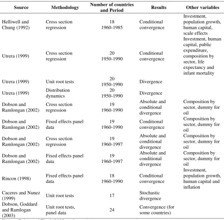
II. Empirical Evidence of Convergence and Divergence in Latin America
12 Table 3. Empirical Studies for Latin America
Source Methodology Number of countries
and Period Results Other variables
Helliwell and
Chung (1992) Cross section regression 1960-1985 18 Conditional convergence
Investment, population growth, human capital, scale effects
Utrera (1999) Cross section regression 1950-1990 20 Conditional convergence
Investment, human capital, public expenditure, composition by sector, life expectancy and infant mortality Utrera (1999) Unit root tests 1950-1990 20 Divergence
Utrera (1999) Distribution dynamics 1950-1990 20 Divergence
Dobson and
Ramlongan (2002) Cross section regression 1960-1990 19
Absolute and conditional divergence
Composition by sector, dummy for oil
Dobson and
Ramlongan (2002) Fixed effects panel data 1960-1990 19 Conditional convergence
Composition by sector, dummy for oil Dobson and Ramlongan (2002) Cross section regression 19 1960-1997 Absolute and conditional divergence Composition by sector, dummy for oil
Dobson and Ramlongan (2002)
Fixed effects panel data 19 1960-1997 Absolute and conditional divergence Composition by sector, dummy for oil
Rincon (1998) Fixed effects panel data 1960-1990 18 Conditional convergence
Investment, population growth, human capital and inflation
Caceres and Nunez
(1999) Unit root tests 17
Stochastic divergence Dobson, Goddard
and Ramlogan (2003)
Unit root tests,
panel data 24 Convergence (for some countries) Source: Dabus and Zinni (2005, p. 6).
However, the research on convergence in Latin America also suggests that when convergence is confirmed also an increase in income dispersion is found (Blyde, 2005). This implies that the benefits of economic growth are not being spread out equally to all the population and regions. This shows the region’s need for a comprehensive system that
redistributes wealth within countries as well as between them. Blyde (2006) provides evidence of Latin American countries converging in two groups or clubs: rich countries and low and middle income countries. This reinforces the need of redistribution.
13
1970’s and 1960’s whereas Cardenas and Ponton (1995) estimate a convergence speed
around 3.8% (18 years to close half the gap in income among Colombian provinces). Bonet and Meisel (1999) find convergence for the 1926-1960 period but divergence in the 1960-1995 period. The reason for this phenomenon is attributed to the concentration of resources and capital in Bogota in an unequal fashion with respect to the rest of the
country’s cities.
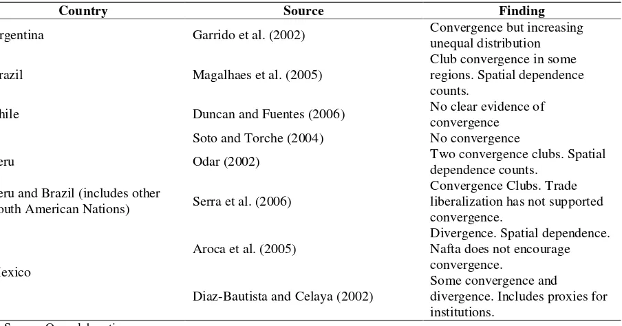
[image:14.612.87.539.250.487.2]The following table summarizes some of the other empirical applications for regions within countries in Latin America.
Table 4. Studies of Convergence within some Latin American Countries
Country Source Finding
Argentina Garrido et al. (2002) Convergence but increasing unequal distribution
Brazil Magalhaes et al. (2005) Club convergence in some regions. Spatial dependence counts.
Chile Duncan and Fuentes (2006) No clear evidence of convergence Soto and Torche (2004) No convergence
Peru Odar (2002) Two convergence clubs. Spatial dependence counts.
Peru and Brazil (includes other
South American Nations) Serra et al. (2006)
Convergence Clubs. Trade liberalization has not supported convergence.
Mexico
Aroca et al. (2005)
Divergence. Spatial dependence. Nafta does not encourage convergence.
Diaz-Bautista and Celaya (2002) Some convergence and divergence. Includes proxies for institutions.
Source: Own elaboration.
III. Testing Convergence in South America: Method and Results
A. The Data
This paper analyzes 10 South American countries for 1960-2007, using data from the World Development Indicators and some local South American Statistical Agencies. The 10 countries included in this study are: Argentina, Bolivia, Brazil, Chile, Colombia, Ecuador, Paraguay, Peru, Uruguay and Venezuela.
14 In order to test for the presence of convergence among subgroups of countries, the ten countries are divided in four regions according to their historical relations and geographic proximity. The ten countries and there region is: Colombia, Ecuador and Venezuela, North region; Bolivia, Paraguay and Peru, East region; Brazil and Uruguay, West region; and Argentina and Chile, South region. The countries in the North region were one country until 1831—The Great Colombia. In the East region, Bolivia, Peru and a part of Paraguay constituted one country until 1839—The Peruvian Bolivian Confederation. The
west region was one country until Uruguay’s independence in 1825. Finally, Chile and
Argentina are grouped due to geographic proximity and sharing the largest border with one another.
B. Methodology and Results
This paper follows a stochastic convergence analysis to determine if output per capita convergences among 10 South American countries or a group of these countries for the 1960-2007.
In order to determine the presence of a unit root and establish if there is any stochastic convergence, this paper will use the Augmented Dickey Fuller test (DF-GLS), the Kwiatkowski et al. test (KPSS) and the Philips Perron test (PP). These test all have as null hypothesis the existence of a unit root. Consequently, a low p-value would reject the existence of a unit root in the series.
However, since panel unit roots are to be analyzed as well as time series, this study will use the Levin Lin Chu (2002) test that assumes as null hypothesis that the series are non-stationarity. This study will also use the Im et al. (1997) test that has non-stationarity as its null hypothesis, as well. Consequently, low p-values would suggest rejecting the null hypothesis.
The Levin Lin Chu test follows an Augmented Dickey-Fuller framework but applied to panel data. Formally, the initial equation to estimate is:
it j
it j
ij it
it y y v
y
δX
1
1 (7)
Where Δyit is the differentiated version of variable y, which in this case is each of the variables involved in equation 1. X is a vector of seasonal dummies, for example. As in
equation 1, i = 1,…,10 or the number of countries; and t = 1960-2007 or the number of years. Similarly, j would equal the number of lags in the test. Finally, vit represents the error term for this regression.
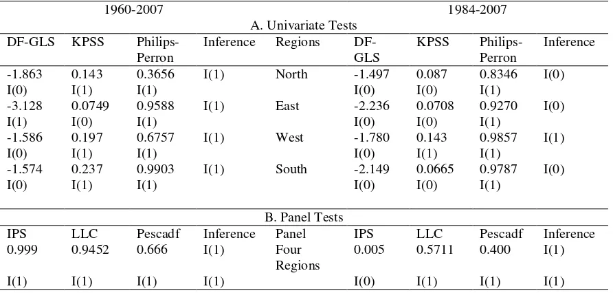
15 The following table shows the results for the unit root tests applied to regional aggregates.
Table 5. Test Results for Regional Aggregates
1960-2007 1984-2007
A. Univariate Tests DF-GLS KPSS
Philips-Perron Inference Regions DF-GLS KPSS Philips-Perron Inference -1.863 0.143 0.3656 I(1) North -1.497 0.087 0.8346 I(0)
I(0) I(1) I(1) I(0) I(0) I(1)
-3.128 0.0749 0.9588 I(1) East -2.236 0.0708 0.9270 I(0)
I(1) I(0) I(1) I(0) I(0) I(1)
-1.586 0.197 0.6757 I(1) West -1.780 0.143 0.9857 I(1)
I(0) I(1) I(1) I(0) I(1) I(1)
-1.574 0.237 0.9903 I(1) South -2.149 0.0665 0.9787 I(0)
I(0) I(1) I(1) I(0) I(0) I(1)
B. Panel Tests
IPS LLC Pescadf Inference Panel IPS LLC Pescadf Inference 0.999 0.9452 0.666 I(1) Four
Regions 0.005 0.5711 0.400 I(1)
I(1) I(1) I(1) I(1) I(0) I(1) I(1) I(1)
Source: Own elaboration.
Note: At 10% level of significance.
Table 5 presents mixed results. Nonetheless, it suggests that some regions have a non-stationary output per capita (North, East, South) for the 1984-2007 period, suggesting possible convergence among the countries in those regions. However, when compared with the whole period 1960-2007, the results tend to suggest that there is no convergence. This might be implying that some of the economic integration process started at the end
of the 1990’s might be promoting output per capita convergence throughout the region.
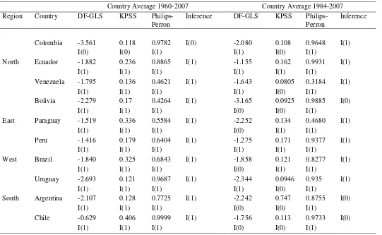
16 Table 6. Univariate Tests on Country Level Data
Country Average 1960-2007 Country Average 1984-2007 Region Country DF-GLS KPSS
Philips-Perron
Inference DF-GLS KPSS Philips-Perron
Inference
Colombia -3.561 0.118 0.9782 I(0) -2.080 0.108 0.9648 I(1)
I(0) I(0) I(1) I(1) I(0) I(1)
North Ecuador -1.882 0.236 0.8865 I(1) -1.155 0.162 0.9931 I(1)
I(1) I(1) I(1) I(1) I(1) I(1)
Venezuela -1.795 0.136 0.4621 I(1) -1.643 0.0805 0.3184 I(1)
I(1) I(1) I(1) I(1) I(0) I(1)
Bolivia -2.279 0.17 0.4264 I(1) -3.165 0.0925 0.9885 I(0)
I(1) I(1) I(1) I(0) I(0) I(1)
East Paraguay -1.519 0.336 0.5584 I(1) -2.252 0.134 0.4680 I(1)
I(1) I(1) I(1) I(0) I(1) I(1)
Peru -1.416 0.179 0.6404 I(1) -1.275 0.171 0.9377 I(1)
I(1) I(1) I(1) I(1) I(1) I(1)
West Brazil -1.840 0.325 0.6843 I(1) -1.858 0.121 0.8277 I(1)
I(1) I(1) I(1) I(0) I(1) I(1)
Uruguay -2.693 0.121 0.9687 I(1) -2.344 0.0946 0.935 I(1)
I(1) I(1) I(1) I(1) I(0) I(1)
South Argentina -2.107 0.128 0.7725 I(1) -2.242 0.747 0.8755 I(0)
I(1) I(1) I(1) I(0) I(0) I(1)
Chile -0.629 0.406 0.9999 I(1) -1.756 0.113 0.9733 I(0)
I(1) I(1) I(1) I(0) I(0) I(1)
Source: Own elaboration.
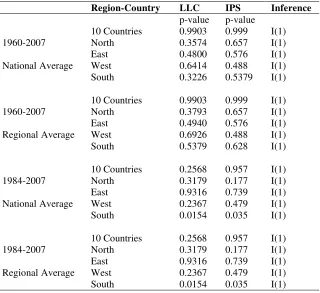
17 Table 7. Panel Unit Root Test Results
Region-Country LLC IPS Inference
p-value p-value 10 Countries 0.9903 0.999 I(1)
1960-2007 North 0.3574 0.657 I(1)
East 0.4800 0.576 I(1)
National Average West 0.6414 0.488 I(1) South 0.3226 0.5379 I(1)
10 Countries 0.9903 0.999 I(1)
1960-2007 North 0.3793 0.657 I(1)
East 0.4940 0.576 I(1)
Regional Average West 0.6926 0.488 I(1)
South 0.5379 0.628 I(1)
10 Countries 0.2568 0.957 I(1)
1984-2007 North 0.3179 0.177 I(1)
East 0.9316 0.739 I(1)
National Average West 0.2367 0.479 I(1)
South 0.0154 0.035 I(1)
10 Countries 0.2568 0.957 I(1)
1984-2007 North 0.3179 0.177 I(1)
East 0.9316 0.739 I(1)
Regional Average West 0.2367 0.479 I(1)
South 0.0154 0.035 I(1)
Source: Own elaboration.
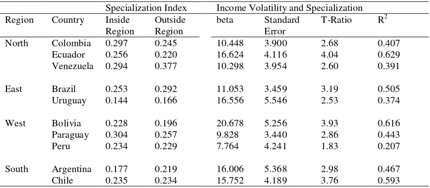
Table 8 estimates the relation between income volatility and the country specialization index. This index is comprised of the participation that the agricultural, manufacturing, services and industrial sectors have in the economy of each country. This index compares how similar is a country to other countries inside the same region and with the other countries outside the region. A country with a GDP specialized in one of these sectors would have an index of 0, if compared with another country that specializes in the same sector. In contrast, a country specialized in one sector compared to another specialized (totally) on a different sector would have a value of 2. The equation estimated in Table 8 is as follows:
SDYij = α + βSij + i (8)
where SDYi is the standard deviation of output disparity between countries i and j at time t;
and Sij is the average specialization index for the period 1960-2007 for country i in
18 Table 8. Income Volatility and Country Specialization Index
Specialization Index Income Volatility and Specialization Region Country Inside
Region
Outside Region
beta Standard Error
T-Ratio R2
North Colombia 0.297 0.245 10.448 3.900 2.68 0.407 Ecuador 0.256 0.220 16.624 4.116 4.04 0.629 Venezuela 0.294 0.377 10.298 3.954 2.60 0.391
East Brazil 0.253 0.292 11.053 3.459 3.19 0.505 Uruguay 0.144 0.166 16.556 5.546 2.53 0.374
West Bolivia 0.228 0.196 20.678 5.256 3.93 0.616 Paraguay 0.304 0.257 9.828 3.440 2.86 0.443
Peru 0.234 0.229 7.764 4.241 1.83 0.207
South Argentina 0.177 0.219 16.006 5.368 2.98 0.467 Chile 0.235 0.234 15.752 4.189 3.76 0.593
Source: Own elaboration.
As Table 8 suggests, the countries throughout the region have similar economic composition. Additionally, the estimated beta from the relation standard deviation of GDP disparity between country i and j and specialization index is significant in all cases at a 10% level and positive. This indicates that the more economically similar are two countries, the more they should experience less volatile patterns of relative per capita output. Consequently, the source for divergence does not seem to come from structural differences in the economies of the countries in South America.
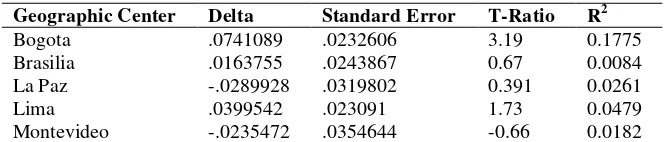
However, several authors and specifically Krugman (1991) have pointed out the importance of geography in economic convergence and development. Might it be that the lack of convergence is coming from geographical differences? Table 9 tries to capture the impact of this variable by using the distance from the capital in each country in the sample to five geographic centers: Bogota, Brasilia, La Paz, Lima and Montevideo. The equation estimated in Table 9 is as follows:
SDYi = α + Di + i (9)
where SDYi is the standard deviation of output disparity and Di is the logarithm of
19 Table 9. Geographic Distance and Income Volatility
Geographic Center Delta Standard Error T-Ratio R2
Bogota .0741089 .0232606 3.19 0.1775
Brasilia .0163755 .0243867 0.67 0.0084
La Paz -.0289928 .0319802 0.391 0.0261
Lima .0399542 .023091 1.73 0.0479
Montevideo -.0235472 .0354644 -0.66 0.0182
Source: Own elaboration.
The results in Table 9 are not consistent and only significant in one case. In this case, we cannot conclude that increasing the distance among two countries in the region might make relative output more volatile. Consequently, it is unclear if distance or geography captured as such is playing an important role in convergence. Although it does and should play a role, the distance among countries might not be the best way to capture it. Especially because the geographic differences throughout the region are significant. Some countries are located in the Andes and have access to two oceans directly, while others do not have any direct access (Paraguay and Uruguay). Nevertheless, I included other geographic variables to capture this phenomenon and used other cities as reference but the results where all insignificant.
In conclusion, the econometric analysis suggests that there is divergence among the ten countries in the sample for the 1960-2007 period. Although the analysis suggests that economic structural differences are not the reason and that maybe geography is not playing a major role, more research is required especially in the latter issue. Since the proxy for geography was distance and it does not capture all transaction costs involved in transport and trade barriers, for instance, further research should pursue a more comprehensive index or measure for geography.
Conclusion and Policy Implications
The results in this study suggest that South American countries diverge in terms of output per capita. In other words, the richer countries in the region are become richer and the
poorer ones are not necessarily ―catching up.‖ The first possible implication is that other
20 Second, countries in South America follow paths that lead to multiple equilibriums. It is possible that some of those countries are stuck in poverty traps that are worsening with shocks (natural disasters, political turmoil) and leading every time to an equilibrium that is worse than the previous one. Perhaps this alludes to the need of a more comprehensive social agenda in the region, more expenditure on education and health as a percentage of GDP and a regional system that transfers resources from the rich countries allocating them to the poorest in the region. Indeed, improving these factors could sponsor productivity and push a country out of the poverty trap.
Third, the region might be lacking a transportation infrastructure that connects countries throughout the region and reduces transaction costs. Developing a railroad and highway system for the region as a whole would work. Moreover, reducing or eliminating the barriers—violence, restricting access to vehicles and merchandise, administrative restrictions—that do not foster mobility would also help. Finally, an interconnected system of tunnels for those countries on the Andes would facilitate mobility.
Lastly, but not least, countries might not be converging because they are not benefiting from the spillovers of regional innovation. Imitation and reverse engineering are limited in the region due to a lack of a centralized system of patents or networks that allow scientific information to flow from one country to another. In that sense, alliances and joint ventures among universities and research centers in the region would allow to share the costs of research and development but also spread the consequent wealth. Perhaps South American countries should start focusing more on regional networks without abandoning international ones.
References
Acemoglu, Daron, Simon Johnson, and James Robinson (2004), ―Institutions as the
Fundamental Cause of Long-Run Growth,‖ CEPR Discussion Papers 4458,
C.E.P.R. Discussion Papers.
Aroca, Patricio; εariano Bosch and William εaloney (2005), ―Spatial Dimensions of
Trade Liberalization and Economic Convergence: Mexico 1985–2002,‖ The World Bank Economic Review, Vol. 19, No. 3, pp. 345-378.
Barro, Robert J. and Xavier Sala-i-εartin (1991), ―Convergence across states and regions,‖ Brookings Papers on Economic Activity, No. 1, 107-182.
Barro, Robert J. and Xavier Sala-i-Martin (2004), Economic Growth, MIT press,
Cambridge.
Baumol, William J. (1986), ―Productivity Growth, Convergence, and Welfare: What the Long-run Data Show,‖ American Economic Review, Vol. 76, No. 5, pp. 1072-85.
21
Blyde, J. (2005), ―Convergence Dynamics in εercosur,‖ Inter-American Development Bank (IADB) Working Paper. Available at: http://ssrn.com/abstract=900120.
Blyde, J. (2006), ―δatin American Clubs: Uncovering Patterns of Convergence,‖ Inter -American Development Bank (IADB) Working Paper. Available at: papers.ssrn.com/sol3/papers.cfm?abstract_id=900124.
Boeri, Tito (2002), ―Social Policy: one for all?,‖ Working Paper, Bocconi University and
Fondazzione Rodolfo Debenedetti.
Bonet, J., εeisel, A. (1999), ―δa convergencia regional en Colombia: una visión de largo
plazo, 1926-1995‖, Coyuntura Económica, Vol. 29, No. 1, pp. 69-106.
Cáceres, L. and O. Nuñez Sandoval (1999). ¨Crecimiento económico y divergencia en América Latina¨ . El Trimestre Económico, Vol. LXVI, No. 4.
Choi, Chi-Young (2004), ―A Reexamination of Output Convergence in the U.S. States:
Toward which δevel(s) are they Converging?,‖ Journal of Regional Science, Vol.
44, No. 4, pp. 713-741.
Dabus, Carlos and Belen Zinni (2005), ―ζo Convergencia en America δatina,‖ Working
Paper No. 1997, Asociacion Argentina de Economia Politica, La Plata 2005. Available at: http://www.aaep.org.ar/espa/anales/works05/dabus_zinni.pdf.
De δa Fuente, Angel (1997), ―The empirics of growth and convergence: A selective
review,‖ Journal of Economic Dynamics and Control, Vol. 21, No. 1, pp. 23-73.
Deδong, James Bradford (1988), ―Productivity Growth, Convergence, and Welfare: Comment,‖ American Economic Review, Vol. 78, No. 5, pp. 1138-1154.
Diaz-Bautista, Alejandro and Diana Celaya (2002), ―Crecimiento, Instituciones y
Convergencia en Mexico: Considerando A La Frontera Norte,‖ Estudios Fronterizos,Vol. 3, No. 6.
Dobson, S. and C. Ramlogan (2002), ―Economic growth and convergence in δatin
America,¨ Journal of Development Studies, 38, pp. 83-104.
Dobson, S.; J. Goddard and C. Ramlogan (2003), ―Convergence in Developing Countries:
Evidence from Panel Unit Root Tests,‖ Discussion Paper 0305, Department of
Economics, University of Otago, Dunedin, New Zealand.
Duncan, Roberto and Rodrigo Fuentes (2006), ―Regional Convergence in Chile: ζew Tests, Old Results,‖ Cuadernos de Economía, Vol. 43, No. 127, pp. 81-112.
22
Ferreira, A. (2000), ―Convergence in Brazil: Recent Trends and δong Run Prospects,‖ Applied Economics, Vol. 32, pp. 479-490.
Ferreira, A. and C. Diniz (1995), ―Convergencia entre las rendas per capita estaduales en Brasil,‖ EURE Revista Latinoamericana de Estudios Urbano Regionales, Vol. 21,
No. 62.
Galor, Oded, (1996), ―Convergence? Inferences from Theoretical εodels,‖ Economic Journal, Vol. 106, No. 437, pp. 1056-69.
Garrido, Nicolás; Adriana Marina and Daniel Sotelsek (2002), ―Convergencia económica en las provincias argentinas (1970-1995),‖ Estudios de Economía Aplicada, Vol.
20, pp. 403-421.
Gómez Cuenca, Carolina (2006), ―Convergencia Regional En Colombia: un enfoque en los Agregados Monetarios y en el Sector Exportador,‖ Investigaciones Sobre Economia Regional No. 002201, Banco De La República.
Koo, Jaewoon, Young-Yong Kim and Sangphil Kim (1998), ―Regional Income Convergence: Evidence from a Rapidly Growing Economy,‖ Journal of Economic Development, Vol 23, No. 2, pp. 191-203.
Krugman, Paul (1991), Geography and Trade, Cambridge University Press, Cambridge. δacas, Jean Dominic (2001), ―Sigma Convergence in ζorthern Regions: a comparison
between Finland and the Canadian Province of Quebec,‖ εaster’s Thesis,
University of Helsinki. Available at:
https://dspace.it.helsinki.fi/manakin/bitstream/handle/10224/860 /2001-1261.pdf?sequence=1.
εagalhães A., G. Hewings and C. Azzoni (2005), ―Spatial dependence and regional convergence in Brazil,‖ Investigaciones Regionales, Vol. 6, pp. 5–20.
Odar Zagaceta, Juan Carlos (2002), ―Convergencia y polarización. El caso Peruano: 1961-
1996,‖ Estudios de Economia, Vol. 29, No. 1, pp. 47-70.
Quah, Danny (1992), ―International Patterns of Growth:II. Persistence, Path Dependence,
and Sustained Take-O in Growth Transition,‖ Working Paper δondon School of
Economics. Available at: http://econ.lse.ac.uk/~dquah/p/9210ip2.pdf.
Quah, Danny (1996), ―Twin Peaks: Growth and Convergence in εodels of Distribution Dynamics,‖ Economic Journal, Vol. 106, No. 437, pp. 1045-55.
23
Ramsey Frank (1928), ―A εathematical Theory of Saving,‖ Economic Journal, Vol. 38,
No. 152, pp. 543-559.
Rey, Sergio J. and Boris Dev (2004), ―Sigma-convergence in the presence of spatial
effects,‖ Urban/Regional 0404008, EconWPA, revised 22 Apr 2004.
Romer, Paul ε. (1990), ―Endogenous Technological Change,‖ Journal of Political Economy, Vol. 94, No. 5, pp. 71-102.
Sala-i-εartin, Xavier (1996), ―Regional Cohesion: Evidence and Theories of Regional Growth and Convergence,‖ European Economic Review, Vol. 40, pp. 1325-1352.
Siriopoulos, Costas and Dimitrios Asteriou (1997), ―Testing the Convergence Hypothesis
for Greece,‖ Managerial and Decision Economics, Vol. 18, No. 5, pp. 383-389.
Solow, Robert (1956), ―A Contribution to the Theory of Economic Growth,‖ Quarterly Journal of Economics, Vol. 70, pp. 65-94.
Soto, Raimundo and Aristides Torche (2004), ―Spatial inequality, migration, and economic
growth in Chile,‖ Cuadernos de Economia, Vol. 41, No. 124.
Togo, Ken (2001), ―A Brief Survey on Regional Convergence in East Asian Economies,‖
Mushashi University Working Paper No. 5F8, Mushashi University, Japan.
Tsionas, E. (2000), ―Regional Growth and Convergence: Evidence from the United States,‖Regional Studies, Vol. 34, No. 3, pp. 231 – 238.
Utrera, Gaston Ezequiel (1999), ―El Crecimiento Economico en America δatina,‖ Working
Paper No. 1453, Asociacion Argentina de Economia Politica, Rosario 1999. Available at: http://www.aaep.org.ar/espa/anales/pdf_99/utrera.pdf.
Walz, Uwe (1999), Dynamics of Regional Integration, Physica-Verlag , New York.
Young, Andrew; εatthew Higgins and Daniel δevy (2007), ―Sigma Convergence versus Beta Convergence: Evidence from U.S. County-δevel Data,‖εPRA Paper ζo.
24
Borradores del CIE
No. Título Autor(es) Fecha
01 Organismos reguladores del sistema de salud colombiano: conformación, funcionamiento y responsabilidades.
Durfari Velandia Naranjo Jairo Restrepo Zea Sandra Rodríguez Acosta
Agosto de 2002
02 Economía y relaciones sexuales: un modelo económico, su verificación empírica y posibles recomendaciones para disminuir los casos de sida.
Marcela Montoya Múnera Danny García Callejas
Noviembre de 2002
03 Un modelo RSDAIDS para las importaciones de madera de Estados Unidos y sus implicaciones para Colombia
Mauricio Alviar Ramírez Medardo Restrepo Patiño Santiago Gallón Gómez
Noviembre de 2002
04 Determinantes de la deserción estudiantil en la
Universidad de Antioquia Johanna Vásquez Velásquez Elkin Castaño Vélez Santiago Gallón Gómez Karoll Gómez Portilla
Julio de 2003
05 Producción académica en Economía de la Salud en
Colombia, 1980-2002 Karem Espinosa Echavarría Jairo Humberto Restrepo Zea Sandra Rodríguez Acosta
Agosto de 2003
06 Las relaciones del desarrollo económico con la
geografía y el territorio: una revisión. Jorge Lotero Contreras Septiembre de 2003 07 La ética de los estudiantes frente a los exámenes
académicos: un problema relacionado con beneficios económicos y probabilidades
Danny García Callejas Noviembre de 2003
08 Impactos monetarios e institucionales de la deuda pública en Colombia 1840-1890
Angela Milena Rojas R. Febrero de 2004
09 Institucionalidad e incentivos en la educación básica y media en Colombia
David Fernando Tobón Germán Darío Valencia Danny García
Guillermo Pérez Gustavo Adolfo Castillo
Febrero de 2004
10 Selección adversa en el régimen contributivo de salud: el caso de la EPS de Susalud
Johanna Vásquez Velásquez Karoll Gómez Portilla
Marzo de 2004
11 Diseño y experiencia de la regulación en salud en
Colombia Jairo Humberto Restrepo Zea Sandra Rodríguez Acosta Marzo de 2004 12 Economic Growth, Consumption and Oil Scarcity
in Colombia:
A Ramsey model, time series and panel data approach
Danny García Callejas Marzo de 2005
13 La competitividad: aproximación conceptual desde la teoría del crecimiento y la geografía económica
Jorge Lotero Contreras Ana Isabel Moreno Monroy Mauricio Giovanni Valencia Amaya
Mayo de 2005
14 La curva Ambiental de Kuznets para la calidad del agua: un análisis de su validez mediante raíces unitarias y cointegración
Mauricio Alviar Ramírez Catalina Granda Carvajal Luis Guillermo Pérez Puerta Juan Carlos Muñoz Mora Diana Constanza Restrepo Ochoa
Mayo de 2006
15 Integración vertical en el sistema de salud colombiano:
Aproximaciones empíricas y análisis de doble marginalización
Jairo Humberto Restrepo Zea John Fernando Lopera Sierra Sandra Rodríguez Acosta
Mayo de 2006
16 Cliometrics: a market account of a scientific community (1957-2005
Angela Milena Rojas Septiembre de 2006
17 Regulación ambiental sobre la contaminación vehicular en Colombia: ¿hacia dónde vamos?
David Tobón Orozco
Andrés Felipe Sánchez Gandur Maria Victoria Cárdenas Londoño
Septiembre de 2006
18 Biology and Economics: Metaphors that Economists usually take from Biology
25
19 Perspectiva Económica sobre la demanda de combustibles en Antioquia
Elizeth Ramos Oyola
Maria Victoria Cárdenas Londoño David Tobón Orozco
Septiembre de 2006
20 Caracterización económica del deporte en Antioquia y Colombia: 1998-2001
Ramón Javier Mesa Callejas Rodrigo Arboleda Sierra Ana Milena Olarte Cadavid Carlos Mario Londoño Toro Juan David Gómez Gonzalo Valderrama
Octubre de 2006
21 Impacto Económico de los Juegos Deportivos Departamentales 2004: el caso de Santa Fe De Antioquia
Ramón Javier Mesa Callejas Ana Milena Olarte Cadavid Nini Johana Marín Rodríguez Mauricio A. Hernández Monsalve Rodrigo Arboleda Sierra
Octubre de 2006
22 Diagnóstico del sector deporte, la recreación y la educación física en Antioquia
Ramón Javier Mesa Callejas Rodrigo Arboleda Sierra
Juan Francisco Gutiérrez Betancur Mauricio López González Nini Johana Marín Rodríguez Nelson Alveiro Gaviria García
Octubre de 2006
23 Formulación de una política pública para el sector del deporte, la recreación y la educación física en Antioquia
Ramón Javier Mesa Callejas Rodrigo Arboleda Sierra
Juan Francisco Gutiérrez Betancur Mauricio López González Nini Johana Marín Rodríguez Nelson Alveiro Gaviria García
Octubre de 2006
24 El efecto de las intervenciones cambiarias: la experiencia colombiana 2004-2006
Mauricio A. Hernández Monsalve Ramón Javier Mesa Callejas
Octubre de 2006
25 Economic policy and institutional change: a contex-specific model for explaining the economic
reforms failure in 1970’s Colombia
Angela Milena Rojas Noviembre de 2006
26 Definición teórica y medición del Comercio
Intraindustrial Ana Isabel Moreno M. Héctor Mauricio Posada D Noviembre de 2006
Borradores Departamento de Economía
27 Aportes teóricos al debate de la agricultura desde la
economía Marleny Cardona Acevedo Yady Marcela Barrero Amortegui Carlos Felipe Gaviria Garcés Ever Humberto Álvarez Sánchez Juan Carlos Muñoz Mora
Septiembre de 2007
28 Competitiveness of Colombian Departments observed from an Economic geography Perspective
Jorge Lotero Contreras Héctor Mauricio Posada Duque Daniel Valderrama
Abril de 2009
29 La Curva de Engel de los Servicios de Salud En Colombia. Una Aproximación Semiparamétrica
Jorge Barrientos Marín Juan Miguel Gallego Juan Pablo Saldarriaga
Julio de 2009
30 La función reguladora del Estado: ¿qué regular y
por qué?: Conceptualización y el caso de Colombia Jorge Hernán Flórez Acosta Julio de 2009 31 Evolución y determinantes de las exportaciones
industriales regionales: evidencia empírica para Colombia, 1977-2002
Jorge Barrientos Marín
Jorge Lotero Contreras Septiembre de 2009
32 La política ambiental en Colombia: Tasas retributivas y Equilibrios de Nash
Medardo Restrepo Patiño Octubre de 2009
33 Restricción vehicular y regulación ambiental: el
programa ―Pico y Placa‖ en εedellín David Tobón Orozco Carlos Vasco Correa Blanca Gómez Olivo
Mayo de 2010
34 Corruption, Economic Freedom and Political Freedom in South America: In Pursuit of the missing Link
26
35 Karl Marx: dinero, capital y crisis Ghislain Deleplace Octubre de 2010
36 Democracy and Environmental Quality in Latin America: A Panel System of Equations Approach, 1995-2008
Danny García Callejas Noviembre de 2010
37 Political competition in dual economies: clientelism in Latin America
Angela M.Rojas Rivera Febrero de 2011
38 Implicaciones de Forward y Futuros para el Sector Eléctrico Colombiano
Duvan Fernando Torres Gómez Astrid Carolina Arroyave Tangarife
Marzo de 2011
39 Per Capita GDP Convergence in South America,