Serie documentos de trabajo
Family Income Inequality and the Role of Wives Earnings in Mexico: 1988-2010
Raymundo M. Campos Vázquez El Colegio de México
Andrés Hincapie Yale University Rubén Irvin Rojas Valdés Inter-American Development Bank
Julio, 2011
Family Income Inequality and the Role of
Wives’Earnings in Mexico: 1988-2010
Raymundo M. Campos-Vazquez
yAndres Hincapie
zRuben Irvin Rojas-Valdes
xThis Version: May 2011 First Version: November 2010
Abstract
We study family income inequality in Mexico from 1988 to 2010. Female labor
supply increased during this period, especially for married women. The share of wives’
income among married couples grew from 13 percent in 1988 to 23 percent in 2010.
However, the correlation of husbands’and wives’earnings has been fairly stable with a
value close to 0.28, one of the highest correlations recorded across countries. We follow
Cancian and Reed’s (1999) methodology in order to analyze whether wives’ income
equalizes total family income distribution. We investigate several counterfactuals and
conclude that the recent increment in female employment has contributed to a decrease
in family income inequality mainly through a rise in wives’labor supply in poor families.
JEL Codes: J12; J21; J31; O15; O54.
Keywords: Income Inequality; Female Employment; Female Earnings; Latin America; Mexico.
We thank Eva O. Arceo-Gómez, James Cameron, Gerardo Esquivel, Anna Isaykina, Julia Rozanova, Isidro Soloaga and Christopher Wildeman for valuable comments. All remaining errors are our own. Andres Hincapie acknowledges …nancial support from the Fox International Fellowiship at Yale University.
yCorresponding author. E-mail: rmcampos@colmex.mx, http://raycampos.googlepages.com. Address:
El Colegio de México, Centro de Estudios Económicos, Camino al Ajusco 20, Pedregal de Santa Teresa, 10740, Mexico DF. Phone: +52-55-54493000, ext. 4153. Fax: +52-55-56450464.
zE-mail: ahincapie@colmex.mx, Address: Fox International Fellowship, Yale University, 34 Hillhouse
Avenue, 06511, New Haven, CT. Phone: +1-203-9315210.
xE-mail: rubenr@iadb.org. Address: Research Fellow, Inter-American Development Bank, Integration
1
Introduction
Latin America is characterized by being a region highly unequal in terms of income (Ferreira
et al. 2003; Lopez and Perry 2008). Mexico is also characterized by large income
inequal-ity: Gini coe¢ cient computations yield a …gure around 0.52 in 2005, the 15th highest of
24 countries in Latin America with comparable data (Lopez and Perry 2008; Lopez-Calva
and Lustig 2010).1 However, since the mid 1980s Mexico has seen two di¤erent trends of
inequality. From the mid 1980s to the mid 1990s inequality in Mexico increased (Cragg and
Epelbaum 1996; Esquivel and Rodríguez-López 2003). But since the mid to late 1990s there
has been a decline in labor income inequality (Esquivel 2009; Esquivel, Lustig and Scott
2010; Robertson 2007). At the same time, female labor force supply has increased
substan-tially, especially for low skilled female workers. For example, from 1996-2010 female labor
supply increased 11 percentage points.2 Among females, wives increased their labor supply
the most. We investigate the e¤ects of this recent increase in female labor supply among
wives and their earnings on the distribution of family income. The goal of the paper is to
analyze whether wives’ earnings in married-couple households and the change in marriage
rates have an equalizing e¤ect on the family income distribution.
There are two commonly used methods to deconstruct changes in family income
distrib-ution and assess the e¤ect of an increase in wives’earnings on family income inequality. A
semi parametric method has been used to analyze changes in observable characteristics of
the family (DiNardo et. al. 1996; Machado and Mata 2005). The other, which we employ
here, is based on decomposing the coe¢ cient of variation in a fashion that separates the
contribution to variation of each income source (Cancian and Reed 1998, 1999; Del Boca
and Pasqua 2003; Amin and DaVanzo 2004).
Using these two methods, previous literature has not reached a consensus whether wives’
1The Gini coe¢ cient in Mexico for 2008 is 0.506 according to the Mexican institute in charge of
mea-suring o¢ cial poverty. See National Council for the Evaluation of Social Development Policy (CONEVAL), http://www.coneval.gob.mx.
earnings have an equalizing e¤ect on the family income distribution. Furthermore, as shown
in section 2, most of the results are from developed countries. Although there is
substan-tial evidence explaining why income inequality has fallen in Latin America (see the report
by Lopez-Calva and Lustig 2009), little is known about changes in family income
distribu-tions and their determinants. Moreover, during the 1988-2010 period marriage rates, family
structure and the structure of wages changed in Mexico. For Latin American countries, little
is known about the correlation of earnings among married couples or how the share of
in-come among family members has changed over time. Hence, this paper makes an important
contribution in closing that gap.
We follow the methodology proposed by Cancian and Reed (1999) to analyze the role
of wives’earnings on the family income distribution for all families. We use repeated
cross-section datasets from urban Mexico during the period 1988-2010. We consider two broad
groups in the analysis: married-couple households and all other households. We study the
e¤ects of wives’earnings on family income for married-couple households and for the whole
population. We estimate family income inequality using equivalence scales under di¤erent
scenarios for the two broad groups mentioned above. First, we use a counterfactual assuming
wives’ earnings are zero across the population. The second counterfactual assumes a
con-stant mean of wives’earnings among married-couple households. The third counterfactual
assumes mean and dispersion of wives’ earnings constant through the period. The fourth
counterfactual adds the assumption that correlation of wives’and other-sources’earnings is
constant over time. The …nal counterfactual considers changes in marriage rates.
We consistently …nd that wives’earnings contribute to equalizing the income distribution.
Counterfactuals related to the wives’income distribution suggest that inequality would have
been larger had di¤erent characteristics of married females (including mean income, standard
deviation, and the correlation between husbands’and wives’income) stayed constant at its
initial level. On the other hand, had marriage rates kept constant at the 1988 level, inequality
increase in labor supply is higher for wives, low-skilled females and especially for wives in poor
families. We also …nd that the correlation between husbands’and wives’earnings has been
fairly stable over time. Furthermore, its value, about 0.28, is among the highest correlations
recorded across developed countries (Pasqua 2008). Hence, family income inequality did not
fall because of a reduction in assortative mating, its decrease is driven by the increase in
wives’labor supply for poor households and also by changes in the wage structure (reduction
in inequality within wives).
The paper is structured as follows. In section 2, we review previous …ndings on whether
females contribute to equalize the income distribution. Section 3 discusses the methodology
proposed by Cancian and Reed (1999) and explains the counterfactuals we use. Section 4
introduces the data as well as some descriptive results. Section 5 presents the main results of
the paper. In section 6 we brie‡y explore possible channels of transmission between female
labor supply and family income inequality. Finally, we conclude in section 7.
2
Literature Review
Social sciences academics have been widely interested in the dynamics of income inequality
and its potential causes. Particularly, the study of wage inequality has been of special interest
among labor economists.3 For the period 1988-2010 in Mexico, income and wage inequality
follow an inverted-U shape pattern (Lopez-Calva and Lustig 2010, and Esquivel, Lustig and
Scott 2010). There has been a substantial number of studies that analyze the potential
causes of change in inequality at the individual level.4 However, little is known about the
3Katz and Autor (1999) and Machin (2008) present a general review of the …ndings regarding the sources
of change in wage inequality. For the U.S. the consensus is that both competitive and non-competitive sources are responsible for changes in the wage distribution. For example, relative wages can change due to supply and demand (competitive factors) but also through changes in the minimum wages and unionization rates.
4For the period of increase in inequality (previous to the mid to late 1990s), Cragg and Epelbaum (1996)
role of wives’earnings on the distribution of family income in Mexico.
The distribution of family income is also an important topic to study. In general, we
observe an increase in female labor force participation across countries over time. The rise
in family earnings due to wives labor supply decision may increase or decrease family income
inequality depending on the evolution of husbands’income and also depending on whether
wives in poor or rich families augmented their participation the most. While inequality at
the individual level may decrease, the e¤ects on family income inequality may not be of
the same magnitude or even move in the opposite way. For instance, Juhn and Murphy
(1997) study the period 1969-1989 in the US and …nd that female employment and earnings
have increased the most for females married to high income males. This change suggests
a process of assortative mating and an increase in family income inequality due to this
process. Nevertheless, Juhn and Murphy (1997) do not analyze the consequences on family
income inequality. Gottschalk and Danziger (2005) document changes in inequality for the
period 1975-2002 in the US showing that male wage inequality and family income inequality
move in general in the same way. They argue that inequality would have increased by more
than it did had other members in the household not increased their hours of work. This
suggests that the increase in female labor force participation o¤sets the e¤ect of increasing
male wage inequality in the U.S. However, Gottschalk and Danziger (2005) do not use any
decomposition method to further investigate their claims.
There are two commonly used methods to decompose changes in family income
distribu-tion. While in the …rst one an inequality index is decomposed, a semi-parametric procedure
is used to analyze changes in observable characteristics in the second method (DiNardo et. al.
1996; Machado and Mata 2005). Cancian and Reed (1998, 1999) decompose the coe¢ cient
of variation to investigate the e¤ects of wives’earnings on the distribution of family income.
They use the Current Population Surveys (CPS) in the US for the period 1968-1995 and
con-clude that changes in wives’labor supply and wives’earnings have caused a decline in family
income inequality. Following a similar methodology, but using a longitudinal dataset, Lehrer
(2000) con…rms the …ndings in Cancian and Reed (1998, 1999). Following DiNardo, Fortin,
and Lemieux (1996), Daly and Valleta (2006) …nd that, on the one hand, family income
inequality has decreased due to female earnings but, on the other, it has increased due to
changes in family structure such as marital status and number of children.5 In sum, di¤erent
studies for the US case conclude that wives’earnings reduce family income inequality.
Similar result have been found for the case of Italy and the United Kingdom. Del Boca
and Pasqua (2003), using a coe¢ cient-of-variation decomposition for the period 1977-1998
in Italy, conclude that wives’earnings have an equalizing e¤ect on the family income
distrib-ution. For the period 1968-1990 in the UK, Davies and Joshi (1998) show that female labor
force participation had a small equalizing e¤ect but created a gap between employed- and
not-employed-wife households. Using cross-country analysis for developed countries, Pasqua
(2008) and Harkness (2010) show that, in general, female earnings reduce family income
inequality.
However, in studies for other countries, researchers have found di¤erent results. For
example, Johnson and Wilkins (2004) analyze the case of Australia in the period 1982-1998
using a semi-parametric decomposition. Although they conclude that changes in the labor
force status of the households’ members increased family income inequality, they do not
di¤erentiate between wife labor force status and other-household-members status. Aslaksen,
Wennemo, and Aaberge (2005) analyze the case of Norway for the period 1973-1997 and …nd
a disequalizing e¤ect of female labor income among married couples. They conclude that
this process is due to a ‡ocking together e¤ect, or an increase in assortative mating. For
the case of Brazil 1977-2007, Sotomayor (2009) …nds that female earnings do not a¤ect the
distribution of income in general terms, but they do play an important role in decreasing
poverty rates. Evidence of the role of female earnings on family income inequality is limited
5Martin (2006) assesses the increasing inequality in the United States in the period 1976 –2000 accounting
for developing countries. In particular, little is known about the role of wives’earnings in
the distribution of family income in Mexico.6
Given the lack of evidence for developing countries and especially for Mexico, the analysis
of the role of wives’earnings in family income inequality is particularly relevant. Our paper
contributes to the literature in at least two di¤erent ways. First, we provide descriptive
analysis on the patterns of marriage rates, family income inequality and female labor supply
patterns. Second, we formally analyze the role of wives’ earnings on inequality using the
methods described by Cancian and Reed (1998, 1999) and compare the results to other
studies in di¤erent countries.
3
Implementation
We follow Cancian and Reed (1998, 1999) in order to estimate the e¤ect of wives’earnings
on family income inequality. We divide families into two broad groups according to the
household head status: married- or cohabitating-couple families (group A); and all the other
families, including married individuals whose partner does not currently live in the household,
single, divorced and widowed individuals (group B). We include the second group in order
to analyze the e¤ect of changing marriage rates on the family income distribution.
Married-couple family income can be decomposed into three sources: husband income, wife income,
and residual income. For group B, we only aggregate income at the family level.
Di¤erent indexes of inequality are employed in the literature. Among those, we use
the coe¢ cient of variation (CV) to analyze the role of wives’ earnings on family income
inequality. As pointed out by Cancian and Reed (1998, 1999), the CV can be decomposed
into di¤erent sources. A useful decomposition for married-couple families is the following:
6See Wong and Levine (1992) for an analysis of the factors a¤ecting women’s participation, García (2001)
CVA2 = Sm2CVm2 +Sw2CVw2+So2CVo2+ 2 mwSmSwCVmCVw
+2 moSmSoCVmCVo+ 2 woSoSwCVoCVw (1)
where Si = Yhm+YYhihw+Yho is the share of income (Yh) in householdh for husbands (m), wives
(w) and other sources (o), and i = m; w; o. CVi is the coe¢ cient of variation for each
group and ij is the correlation coe¢ cient between income source i and j. CVA denotes the
coe¢ cient of variation for married couples.
On the other hand, even though the Gini coe¢ cient may be decomposed into di¤erent
sources as well, it has two main disadvantages (Cancian and Reed 1998, 1999). First, the
coe¢ cient itself is problematic when one source is added or omitted. For example, the
Gini coe¢ cient using family income minus wives’income is di¤erent to the Gini coe¢ cient
obtained from the Gini decomposition that dismisses the wives’income component. Second,
and more important, the contribution of a single income source to income inequality cannot
be meaningfully assessed using the Gini decomposition largely because the terms in the
decomposition are not independent of the whole family income distribution.7 In other words,
the Gini coe¢ cient lacks a reference distribution.8 We employ theCV to analyze inequality
trends and the dynamics of wives’income, because it allows us to compare our results against
a reference distribution. We can also interpret the e¤ects of changes in one of the income
sources with respect to the reference distribution.
Equation (1) refers to only married-couple households. We use an additional
decomposi-7The Gini decomposition can be written as G= S
mRmGm+SwRwGw+SoRoGo, where k =m; w; o
refer to the income source,S to the share of income,Rk is the Gini correlation between income sourcekand
total income, and Gk is just the Gini coe¢ cient for the income source k. R is the total correlation which
includes wives’income in the de…nition of total income. Moreover, if we assume wives’earnings equal to zero (SwRwGw= 0), and calculate the Gini coe¢ cient asSmRmGm+SwRwGw+SoRoGo, the result is di¤erent
to the Gini coe¢ cient obtained from total income minus wives’income.
8Cancian and Reed (1998) provide an excellent example to clarify the point: "Consider the hypothetical
tion for the CV in order to include all families in the sample. If we have two broad groups
(married-couple families and other families), the CV in the sample is given by
CV2 = A YA
Y 2
CVA2+ B YB
Y 2
CVB2+
"
A
YA
Y 2
+ B YB
Y 2#
=Y (2)
where is the proportion of families in each group, and Y is the group’s average income.
Hence, it is possible to calculate the contribution of each component and create
counter-factual trends of what would have happened had one component behaved di¤erently. For
example, parameter B measures the percentage of all families but married-couple families.9
In the last 20 years, the percent of married-couple families has decreased in Mexico. We can
ask, then, what would have happened to family income inequality had marriage rate kept
constant at its 1988 level. This counterfactual is easily created by keeping constant B for
every year in the calculation.
The main insight in Cancian and Reed (1998, 1999) is that we can create many
coun-terfactuals and analyze the role of wives’earnings. In this paper, we evaluate …ve di¤erent
counterfactuals for married-couple households as well as for all households:
1. Counterfactual 1. Wives’income is constant, wives show no earnings.
2. Counterfactual 2. Wives’income is constant, their income is equal to the mean value
of a reference distribution.
3. Counterfactual 3. Mean and dispersion of wives do not change over time.
4. Counterfactual 4. Mean, dispersion and correlation of wives’with other
sources’earn-ings do not change over time.
9All families but married-couple families include married individuals whose partner does not currently
5. Counterfactual 5. The percent of married-couple households does not change over
time.10
All counterfactuals are easily calculated plugging-in speci…c values in equations (1)-(2).
For example, in order to obtain counterfactual 1 we can either replace wives’earnings with
zero in our micro data and re-calculate the CV or we can set Sw = CVw = 0. The fact
that both ways give the same answer gives the CV a great advantage over other inequality
indexes. Counterfactual 1 is di¤erent from counterfactual 2 because the dispersion of income
changes. In counterfactual 1, dispersion is equal to zero by de…nition, while in the second case
dispersion is …xed at some positive value. Counterfactual 3 is important because it allows us
to determine whether dispersion among wives equalizes family income distribution. Similar
interpretations follow for the rest of the counterfactuals.
The interpretation of the counterfactuals is straightforward. Using the initial year as the
base year, if inequality in counterfactuals 1 to 4 is higher than observed inequality, then it
is possible to conclude that wives’earnings have an equalizing e¤ect on the family income
distribution. Counterfactual 5 implies the calculation of inequality holding the marriage rate
constant to a base year. If the percent of married-couple families declined over time and
the counterfactual suggests a lower level of inequality using the initial year as the base year,
then it is possible to conclude that the reduction in marriage rates is a disequalizing force
a¤ecting the family income distribution. We analyze the results for both married-couple and
all families. Finally, it is worth noting that the main limitation of our analysis is that we
cannot account for a family member’s labor supply response to changes in the labor supply
of another member.
10We de…ne a married-couple family as that in which either both the husband and wife live together, or
4
Data and Descriptive Statistics
We use data from the households surveys provided by the Mexican statistical o¢ ce
(IN-EGI).11 In particular, we use the following labor force surveys: the Encuesta Nacional de
Empleo Urbano, 1987-1994; Encuesta Nacional de Empleo, 1995-2004; and Encuesta
Na-cional de Ocupación y Empleo, 2005-2010.12 Although some questions of the survey change
from one survey to other, socioeconomic variables, such as age, education, marital status,
monthly labor income and weekly working hours are always comparable. In each survey,
information regarding all household members is recorded. We refer to all surveys as the
labor force surveys.13;14
According to INEGI, a household is a group of one or more people living in a house sharing
expenses (individuals in the household may or may not be relatives). Following Cancian and
Reed (1999), the unit of analysis is the family, not the household that is interviewed. Hence,
we employ a di¤erent de…nition of household in order to isolate household members who are
not relatives of the household head. We de…ne a new household code to account for those
individuals and consider them as an individual household.15
In order to derive some descriptive statistics, we focus on four main samples of families.
First, we consider married couples, their children, and other relatives living in the same
household. This group is comparable with the sample of married couples in Cancian and
Reed (1998, 1999). For each household, we compute the family income as the sum of all
11Data available at http://www.inegi.org.mx
12Surveys contain registers for over 100,000 households, which is especially useful given the number of
di¤erent categories we use in the paper. We use only the second quarter because ENE is national represen-tative only for that quarter. We use only the urban sector (de…ned as municipalities with more than 100,000 inhabitants) because ENEU is by de…nition an urban survey. So, in order to cover the longest period in the analysis, our sample limits to the urban segment (between 40 and 50 percent of the whole population) in the second quarter of each year. These surveys are comparable in general to the ones carried out by the CPS.
13Another survey traditionally used for Mexico is the Household Expenditure-Income Survey (ENIGH).
However, ENIGH is not available every year since 1988, and the sample sizes are considerably lower. A larger sample size is useful because we divide the population by type of household as speci…ed in the text.
14Although we present the main results for the urban sample starting in 1988, we also estimate the results
(not reported) using the national sample starting in 1995. Results are similar for both samples.
15In practice, this change is innocuous given that individuals who are not relatives of the household head
family members’ labor income. We identify husbands’ income, wives’ income and other
sources’income.
Instead of analyzing the rest of the population as one single group, we de…ne three groups
of families in order to understand which of them are non-married-couple families. Firstly, we
broaden the de…nition of household of the original survey to include single headed households,
their children and relatives living in the household. Secondly, we de…ne a group that consists
of those heads who declare to be married or cohabitating but whose spouses do not live in the
household (plus their children and relatives). The …nal group consists of those people living
alone (singles, divorced, separated and widows) or that are not relatives of the household
head. We consider each of those groups a single family. For these households, we only
compute the total family income since there is no spouse present. In order to avoid outliers
with the income measure, we follow the standard literature on wages and trim labor income
to the 0.05 and 99.5 percentiles respectively.
We drop those individuals whose relationship with the household head is not speci…ed
and those with missing information about their education, age, marital status, and household
head status. We also drop all households (and their members) that declare more than one
head or more than one spouse.16 Additionally, we only keep households in which the head
is at least 18 years old and less than 65 years old. Finally, we only use information on
households that declare positive labor income.
Comparing total income across all families may be inadequate due to family size scale
e¤ects. Most of the studies that deal with family income use a general equivalence scale to
adjust for family size. Since the equivalence scale used in studies for other countries may not
be suited for a developing country like Mexico, we use the equivalence scale published by
the National Council for the Evaluation of Social Development Policy (CONEVAL).17 The
equivalence scale gives a weight of 0.70 to individuals 0-5 years old, 0.74 to individuals 6-12
16Dropped observations represent less than 3 percent of each year’s survey.
17This government o¢ ce is in charge of measuring and reporting o¢ cial statistics about poverty rates in
years old, 0.71 to individuals 13-17 years old, and 0.99 to the rest.
[Table 1 here]
Table 1 includes the number of observations at the individual and family level and
de-scriptive statistics for year 1988, 1996, 2004 and 2010. Panel A shows information at the
individual level for the age group 18-65. Mean age has continuously increased over time
from 33 to 36 years, the proportion of married individuals has decreased over time, although
the decline in marriage rates is sharper in the last decade. The proportion of women
work-ing increased from 0.4 in 1988 to 0.57 in 2010. As in previous …ndwork-ings (Esquivel 2009;
Lopez-Acevedo 2006), we can see that inequality follows an inverted-U-shaped pattern. This
pattern is similar both when we calculate inequality at the individual level and at the
fam-ily level. Panel B shows that the proportion of married-couple families has not declined
as much as the proportion of married individuals. The number of individuals less than 18
years old declined substantially in the last 20 years due to a decrease in fertility rates. Mean
income (adjusted by equivalence scales) decreased for the period 1988-1996 (due to the 1995
macroeconomic crisis) and then it increased.
[Figure 1 here]
Figure 1 depicts the percent of families in each of the four types previously described.
The proportion of married-couple families decreased 7 percentage points in the last 20 years.
The percent of households in which one spouse is not present, which represents only a small
fraction (less than 2 percent) of the total, barely changed. On the other hand, the number of
families conformed by one individual, headed by divorced, separated, or widowed individuals
increased (driven mainly by single families).
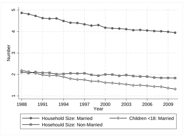
Figure 2 shows the family size for di¤erent types of families. For married-couple families,
it decreased approximately by one member in the last 20 years. This is mainly driven by
On the other hand, family size for all other families has kept fairly constant at around 2
members per family.
[Figure 2 here]
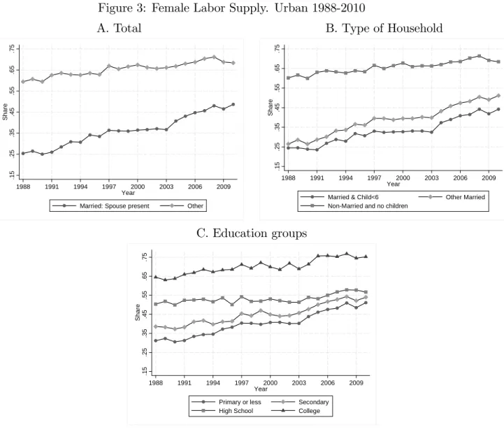
[Figure 3 here]
Figure 3 portrays the patterns of female labor supply for di¤erent groups. Panel A shows
that female labor supply increased relatively more for wives than for non-married females.
For example, wives increased their labor supply by more than 20 percentage points while
for non-married females the rise was close to 10 percentage points. Panel B shows the
patterns of female labor supply for wives with children (less than 6 years old) and other
wives, as well as for non-married females with no children. The increase in female labor
supply is more pronounced among wives with no children. When we calculate labor supply
by education group (panel C), we …nd a rapid increase in female labor supply for females
with low education. Females with completed primary (less than 9 years of schooling) or
completed secondary school (greater than 8 and less than 12 years of schooling) increased
their labor supply more rapidly than females with high school or college degrees.
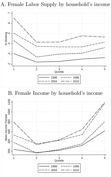
[Figure 4 here]
Figure 4 shows the proportion of women working and mean wives’ income ranked by
household’s income. The x-axis in both panels corresponds to the quintile of family
equiva-lent income distribution once we take out wives’income. Panel A suggests that families with
low family income have a higher proportion of wives working. However, as family income
in-creases (quintile 2 and above), the percent of working wives remains almost the same. There
are some important di¤erences across time. From 1988 to 1996, there is a higher increase
in the percent of working wives in high income households than wives in middle income
households. After 1996, wives in quintiles 1 to 4 increased their labor force participation
Panel B shows the mean wife income for each quintile of the family income distribution. It
shows that mean income in quintile 1 is higher than in quintile 2 due to the high attachment
of wives to the labor market. Wives in rich families earn relatively more than in families in
quintile 2 to 4. In general, Figure 4 shows that women married to men in quintile 5 have not
increased their labor supply as other wives after 1996. Moreover, from 1988 to 1996 there
was a marked increased in earnings for wives in high income households. Also, in the period
1996-2010 there was a higher relative increase in income for wives in quintiles 1-4 than that
for wives in quintile 5.
In sum, previous results show that female labor supply increased in the last 20 years.
This rise is particularly relevant for wives and for females with low education. Additionally,
wives in high income families increased their labor force participation and earnings relatively
more during the period 1988-1996 than in 1996-2010. The next sections show the formal
calculations investigating the e¤ect of wives income on family income inequality.
5
Results
In this section, we show the calculations of the counterfactual analysis described in section 3.
The key parts of those decompositions are the share of income for wives and husbands and
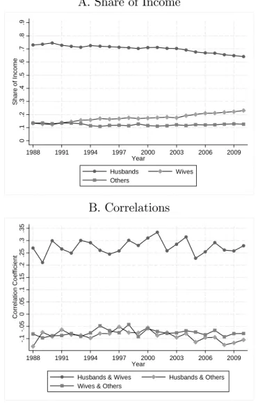
the correlation between income sources. Figure 5 shows these key elements among married
families. The income share of husbands in 1988 is 73 percent while in 2010 it is 64 percent.
At the same time, the income share of wives increased 10 percentage points (from 13 percent
in 1988 to 23 percent in 2010). The income share of other members in the household did not
changed in the last 20 years. Although the income share for wives in the 2000s is similar to
previous …ndings in other countries such as Spain, Greece and Italy (Pasqua 2008; Harkness
2010), it is still substantially lower than in countries such as Denmark and Sweden.18
Panel B in Figure 5 shows that the correlation among income sources have barely changed
18Pasqua (2008) reports a female income share among married couples of 34.5 percent in Denmark and
in the last 20 years. Although the correlations ‡uctuate every year, the long-run relationships
are stable. The correlation between husbands’and wives’income is positive and, on average
across time, equal to 0.28 (in 1988 it is equal to 0.27 and in 2010 to 0.28). This number is
high in comparison to the results of studies for other countries. For the US, Cancian and
Reed (1999) …nd that the correlation between husbands’and wives’income is close to 0.22
in 1994, and they also show an increase in the correlation equal to 0.10 from 1967 to 1994.
Moreover, Del Boca and Pasqua (2003) …nd that the correlation in Italy in 1998 is 0.21,
although they show a correlation of 0.26 for North Italy. Also, Pasqua (2008) shows that
the correlation between husbands’ and wives’ income across OECD countries is fairly low
and close to zero, only Portugal has a correlation close to 0.30. Amin and DaVanzo (2004)
…nd a correlation value equal to 0.13 in 1988 in Malaysia. Hence, a correlation of 0.28 is
larger than those in the U.S., Italy, Malaysia and most OECD countries. As far as we are
concerned, this result for Mexico was not previously known. On the other hand, both the
correlation of husbands’and other sources’income and the correlation of wives’and others
sources’income are close to -0.08.
[Figure 5 here]
[Figure 6 here]
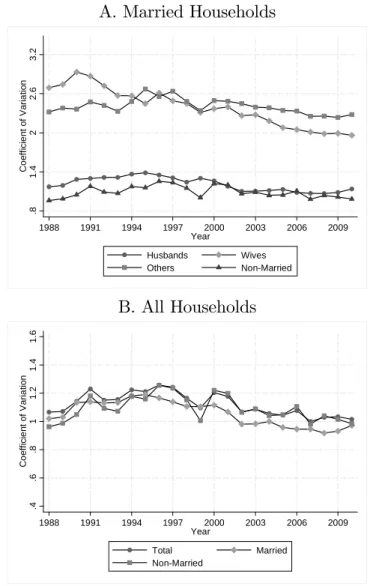
Figure 6 shows the evolution of family income inequality using the coe¢ cient of variation
for each source of income among married-couple families and for all families. Panel A shows
inequality for husbands, wives, other sources and families formed of not-married individuals.
Inequality decreased the most for husbands and wives. Inequality for other sources barely
changed and inequality for not-married individuals slightly decreased for the period
1996-2010. Panel B shows the pattern of inequality for both married-couple and
non-married-couple families. Inequality for married-non-married-couple families decreases substantially after 1996.
This suggests that the fall in family income inequality is mainly driven by the fall in inequality
for husbands and wives income. However, we need formal counterfactuals in order to account
family income inequality during the period 1988-2010. This pattern is robust to changes in
the inequality index or by calculations at the individual level.19
[Figure 7 here]
Now we present the results of the counterfactual computations described in Section 3.
Each counterfactual facilitates our understanding of the role of wives’earnings in inequality.
For example, we say that wives’ earnings contribute to equalize the income distribution if
observed inequality is less than what it would have been had we set wives’income to be zero
or to be the mean value of a reference distribution.
Figure 7 shows the evolution of family income inequality for both married-couple families
and all families in urban areas of Mexico using the observed and counterfactual distributions.
Under this counterfactual, all wives’earnings are equal to zero. The coe¢ cient of variation is
transformed into an index such that 1988 is the base year. If wives had zero earnings across
time, family income inequality would have been larger than observed inequality. Hence,
wives’earnings have an equalizing e¤ect on the income distribution.
[Table 2 here]
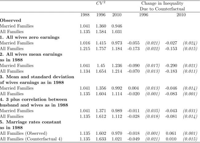
Table 2 shows the main results of the paper for all the counterfactuals previously
dis-cussed. We use 1988 as the base year in our calculations.20 The table presents the results
for years 1988, 1996 and 2010 for the observed coe¢ cient of variation (squared) and the
respective counterfactual. The table includes results for both married-couple families and all
families. Counterfactual 1 assumes earnings of all wives equal to zero. Under this scenario,
inequality for married and all families would have been larger than observed inequality in
1996 and 2010. The last two columns show the di¤erence between observed inequality and its
19See the results by Esquivel (2009), Esquivel, Lustig, and Scott (2010), Lopez-Calva and Lustig (2010),
López-Acevedo (2006) and Campos-Vazquez (2010).
20Using the initial year as the base year is more intuitive than using others. However, our results are
counterfactual. For both years 1996 and 2010, counterfactual 1 implies that wives’earnings
equalize the income distribution. Under this counterfactual, inequality for married females
would have been 0.055 points higher in 1996 and 0.027 points higher in 2010. This means
that in 2010, inequality for married-couple families would have been approximately 3 percent
larger, and around 15 percent larger for all families. The table includes standard errors in
parenthesis for each di¤erence using 500 bootstrap simulations. For counterfactual 1, results
are signi…cant only for the group of all families and not for the group of married-couple
families.
The next rows in Table 2 show the rest of the counterfactuals. Counterfactuals 2-4 show
that wives’earnings have an equalizing e¤ect on the income distribution of married-couple
families and all families. The contribution of wives’ earnings is more pronounced in 2010
than it was in 1996. This is consistent with the increase in female labor supply, especially
for wives, shown in Figure 3. Counterfactual 2 keeps constant wives’ earnings at its 1988
mean value. In this case, inequality would have been larger than its actual value. By 2010,
inequality would have been 30 percent larger among married-couple families and 18 percent
larger among all families. The results are statistically signi…cant.
Counterfactuals 3 and 4 keep the standard deviation of wives’earnings and the correlation
between husbands’and wives’income constant to their 1988 values. Our series of inequality
from both counterfactuals are very similar, which is consistent with the result in Figure 5
showing a fairly stable correlation of earnings between husbands and wives over time. Under
these scenarios, although wives contribute to equalizing the income distribution, they do it
by a less margin than they do under counterfactual 2. This di¤erence is due to a fall in
inequality among wives’earnings over time (Figure 6).
The last counterfactual implies changing the marriage rates among the population. In
this case, we can simulate what would have happened to total family income inequality had
the marriage rate been constant at its 1988 level. We can also simulate what would have
wives’earnings, and the correlation of earnings between husbands and wives been constant
at their 1988 level. Both results are presented in the last rows of Table 2. Had marriage
rates been constant at their 1988 level, family income inequality for all families would have
been lower in 2010. This is due to a fall in inequality among married-couple families. On the
other hand, if we also keep constant the mean and standard deviation of wives’earnings and
also the correlation of earnings among husbands and wives at their 1988 level, inequality for
all families would have decreased only marginally. This means that the change in inequality
generated for the change in wage structure (mean, standard deviation, and correlation) for
wives is cancelled out by the one generated for the change in the marriage rates in the last
20 years.
6
How do females a¤ect the income distribution?
The previous section showed that married female earnings contribute to equalize the income
distribution, especially in the period 1996-2010. In Section 4 we showed that female labor
supply has increased over time, especially for wives (Figures 3 and 4). We also showed
that female labor supply increased relatively more for low-skilled groups. In this section, we
brie‡y analyze how married females a¤ect the income distribution.
[Table 3 here]
Table 3 shows how di¤erent characteristics have evolved over time. As previously shown,
married females have increased their labor supply over time. However, this could be due to
an increase in non-working husbands. The …rst three rows in the table present the percent
of families according to husband and wife working status. Indeed, the percent of families in
which both husband and wife work has been growing in the last 20 years. The percent of
families in which both husband and wife worked in 1988 was 23 percent, but by 2010 this
…gure increased up to 43 percent. The next three rows show that the increase in female
Is this increase in female labor supply related to changes in husbands’income or husbands’
working hours? Results presented in Table 3 show that this is not the case. Both correlations
(rows 8 and 9) are close to zero. Hence, the increase in female labor supply does not seem
to be related to changes in husbands’ employment conditions. It is also possible that the
increase in wives’labor supply is due to new cohorts. If this is the case, we should observe
a decrease or a di¤erentiated pattern in age between wives that work and do not work.
However, Table 3 shows that changes in average age over time for wives that work and do
not work are very similar. This suggests that the increase in female labor supply is not
restricted to younger cohorts.
Table 3 also shows the percent of families in which both husband and wife work, relative
to a speci…ed quartile of the income distribution (excluding wives’income). This percentage
increased more for richer families during the period 1988-1996. However, the gap diminished
in the period 1996-2010. The percent of families in which both husband and wife work in the
…rst quartile increased 15 percentage points during 1996-2010, while for the fourth quartile
it only increased 11 points. Moreover, the last two rows in the table show a marked increase
in the share of income for wives in poor families (…rst quartile), it goes from 13 percent in
1988 to 41 percent in 2010.21 Based on these …ndings and also those in Figures 3 and 4,
we consider that the increase in wives’ labor supply, especially from low income families,
contributed to the decrease in family income inequality.
7
Conclusions
Income inequality in Mexico has followed an inverted-U-shaped pattern in the last 25 years.
At the same time, female labor force participation increased substantially, especially for low
21The increase in the share of income may be due to a higher proportion of non-working husbands. When
skilled female workers. We analyze whether changes in wives’ earnings in married-couple
families and marriage rate changes had an equalizing e¤ect on the family income distribution.
Using data from urban zones in Mexico for the period 1988-2010, we compare observed
family income inequality (using equivalence scales) with counterfactual distributions under
a number of di¤erent assumptions. Our four counterfactuals on income distribution include
assumptions such as zero wive’s income, wive’s income equal to the mean value of a reference
distribution, constant mean and dispersion of wives’s income, and constant correlation of
wives’with other sources’earnings. Additionally, the marriage rate is assumed to be constant
in the …fth counterfactual.
We consistently …nd that wives’earnings equalize the family income distribution.
Coun-terfactuals related to the wives’income distribution suggest that inequality would have been
larger had di¤erent characteristics (such as mean income, standard deviation, and the
cor-relation between husbands’and wives’income) remain constant at their initial level. On the
other hand, had marriage rates kept constant at the 1988 level, inequality would have been
lower.
Although female labor supply augmented for all groups, the rise was higher for wives,
low-skilled females, and wives in poor families. We also …nd that the correlation between
husbands’and wives’earnings has been fairly stable at around 0.28 which is one of the highest
values recorded in similar studies. Hence, we consider that family income inequality did not
fall because of a reduction in assortative mating, its decrease is driven by the increment in
wives’labor supply for poor households and also by changes in the wage structure (reduction
of inequality among wives).
One …nal caution has to be noted. We only consider the e¤ect of market female labor
supply but we neglect the importance of housework. Our data does not allow us to check
whether total hours of work for wives (market plus housework) has changed over time. Hence,
we are unable to point out possible welfare e¤ects at the family level. Although the welfare
participation of wives in the labor market occurs at the expense of their leisure time if wives
remain the principal responsible for housework and childcare. Future research is needed in
References
Amin, S.,andJ. DaVanzo(2004): “The Impact of Wives’Earnings on Earnings Inequality
among married-couple households in Malaysia,”Journal of Asian Economics, 15(1), 49–
70.
Aslaksen, I., T. Wennemo, and R. Aaberge (2005): “’Birds of a Feather Flock
To-gether’: The Impact of Choice of Spouse on Family Labor Income Inequality,”Labour,
19(3), 491–515.
Bosch, M., and M. Manacorda (2008): “Minimum Wages and Earnings Inequality in
Urban Mexico: Revisiting the Evidence,”CEP Discussion Paper 880, Centre for Economic
Performance.
Campos-Vazquez, R. M. (2010): “Why did Wage Inequality decrease in Mexico after
NAFTA?,” Serie Documentos de Trabajo 15, El Colegio de México, Centro de Estudios
Económicos.
Cancian, M., and D. Reed (1998): “Assessing the E¤ects of Wives’Earnings on Family
Income Inequality,”The Review of Economics and Statistics, 80(1), 73–79.
(1999): “The Impact of Wives’ Earnings on Income Inequality: Issues and
Esti-mates,”Demography, 36(2), 173–184.
Cragg, M., and M. Epelbaum (1996): “Why has Wage Dispersion Grown in Mexico? Is
it the Incidence of Reforms or the Growing Demand for Skills?,”Journal of Development
Economics, 51(1), 99–116.
Daly, M. C., and R. G. Valleta (2006): “Inequality and Poverty in the United States:
The E¤ects of Rising Dispersion of Men’s Earnings and Changing Family Behaviour,”
Davies, H., and H. Joshi (1998): “Gender and Income Inequality in the UK 1968-1990:
the Feminization of Earnings or of Poverty?,”Journal of the Royal Statistical Society.
Series A (Statistics in Society), 161(1), 33–61.
Del Boca, D., and S. Pasqua (2003): “Employment Patterns of Husbands and Wives
and Family Income Distribution in Italy (1977-98),”Review of Income and Wealth, 49(2),
221–245.
DiNardo, J., N. M. Fortin, and T. Lemieux (1996): “Labor Market Institutions and
the Distribution of Wages, 1973-1992: A Semiparametric Approach,”Econometrica, 64(5),
1001–1044.
Esquivel, G. (2009): “The Dynamics of Income Inequality in Mexico since NAFTA,”
Regional Bureau for Latin America and the Caribbean Research for Public Policy Inclusive
Development Working Paper ID-02-2009, United Nations Development Programme.
Esquivel, G., N. Lustig, andJ. Scott(2010): “Mexico: A Decade of Falling Inequality:
Market Forces or State Action?,” in Declining Inequality in Latin America. A Decade of
Progress?, ed. by L. F. Lopez-Calva,and N. Lustig, chap. 7, pp. 175–217. United Nations
Development Programme (New York, NY) and Brookings Institution (Washington, DC).
Esquivel, G., and J. A. Rodríguez-López (2003): “Technology, Trade and Wage
In-equality,”Journal of Development Economics, 72(2), 543–565.
Fairris, D.(2003): “Unions and Wage Inequality in Mexico,”Industrial and Labor Relations
Review, 56(3), 481–497.
Ferreira, F., D. De Ferranti, G. E. Perry, and M. Walton (2004): Inequality in
Latin America: Breaking with History? World Bank (Washington DC).
García, B. (2001): “Reestructuración Económica y Feminización del Mercado de trabajo
Gottschalk, P., and S. Danziger (2005): “Inequality of Wage Rates, Earnings and
Family Income in the United States, 1975-2002,”Review of Income and Wealth, 51(2),
231–254.
Harkness, S.(2010): “The Contribution of Women’s Employment and Earnings to
House-hold Income Inequality: A Cross Country Analysis,”Luxembourg Income Survey Working
Paper Series 531, Luxembourg.
Johnson, D., and R. Wilkins (2004): “E¤ects of Changes in Family Composition and
Employment Patterns on the Distribution of Income in Australia: 1981-1982 to
1997-1998,”Economic Record, 80(249), 219–238.
Juhn, C., and K. M. Murphy (1997): “Wage Inequality and Family Labor Supply,”
Journal of Labor Economics, 15(1), 72–97.
Katz, L., and D. Autor (1999): “Changes in the Wage Structure and Earnings
Inequal-ity,” in Handbook of Labor Economics, ed. by O. Ashenfelter, and D. Card, vol. 3C, pp.
1463–1555. North Holland (Amsterdam).
Lehrer, E. L.(2000): “The Impact of Women’s Employment on the Distribution of
Earn-ings among married-couple households: a comparison between 1973 and 1992-1994,”The
Quarterly Review of Economics and Finance, 40(3), 295–301.
Lopez, J. H., and G. Perry (2008): “Inequality in Latin America: Determinants and
Consequences,” Policy Research Working Paper 4504, The World Bank.
Lopez-Calva, L. F., and N. Lustig (2009): “The Recent Decline of Inequality in Latin
America: Argentina, Brazil, Mexico and Peru,” Working Papers 140, ECINEQ, Society
for the Study of Economic Inequality.
(2010): “Explaining the Decline in Inequality in Latin America: Technological
Amer-ica. A Decade of Progress?, ed. by L. F. Lopez-Calva, and N. Lustig, chap. 1, pp. 1–
24. United Nations Development Programme (New York, NY) and Brookings Institution
(Washington, DC).
López-Acevedo, G. (2006): “Mexico: Two Decades of the Evolution of Education and
Inequality,” World Bank Policy Research Working Paper 3919, The World Bank.
Machado, J. A. F., and J. Mata (2005): “Counterfactual Decomposition of Changes in
Wage Distributions using Quantile Regression,”Journal of Applied Econometrics, 20(4),
445–465.
Machin, S. (2008): “An Appraisal of Economic Research on Changes in Wage Inequality,”
Labour, 22(Special Issue), 7–26.
Martin, M. A.(2006): “Family Structure and Income Inequality in Families with Children,
1976 to 2000,”Demography, 43(3), 421–445.
McKenzie, D. J. (2003): “How do Households Cope with Aggregate Shocks? Evidence
from the Mexican Peso Crisis,”World Development, 31(7), 1179–199.
Pasqua, S. (2008): “Wives’Work and Income distribution in European Countries,”
Euro-pean Journal of Comparative Economics, 5(2), 157–186.
Rendón, T. (2003): “Empleo, Segregación y Salarios por Género,” in La Situación del
Trabajo en México, 2003, ed. by E. de la Garza Toledo, and C. S. Páez, chap. VI, pp.
129–150. Plaza y Valdés, S.A. de C.V.
Robertson, R. (2007): “Trade and Wages: Two Puzzles from Mexico,”The World
Econ-omy, 9(30), 1378–1398.
Sotomayor, O. J. (2009): “Changes in the Distribution of Household Income in Brazil:
Wong, R.,andR. E. Levine(1992): “The E¤ect of Household Structure on Women’s
Eco-nomic Activity and Fertility: Evidence from Recent Mothers in Urban Mexico,”Economic
Table 1: Descriptive Statistics
1988 1996 2004 2010 A. Individuals (18-65)
Age 33.9 34.4 35.9 36.8 Married 0.59 0.58 0.55 0.48 % Women Working 0.40 0.46 0.51 0.57 Hourly Wage 31.5 29.5 36.9 34.1 Monthly Income 3375 3238 4319 3970
CV2 (Hr Wage) 0.87 1.09 0.96 0.92 Gini (Hr Wage) 0.40 0.46 0.43 0.41 N 77757 163113 120990 104503 B. Family
% Married 0.71 0.72 0.68 0.64 # Kids (<18) 1.71 1.41 1.15 0.97 Equivalent Income 2803 2685 3622 3420
CV2 (Equiv. Income) 1.13 1.26 1.12 1.03 Gini (Equiv. Income) 0.44 0.49 0.45 0.43 N 32477 68216 52684 46438
Table 2: Main Results under di¤erent Counterfactuals
CV2 Change in Inequality Due to Counterfactual 1988 1996 2010 1996 2010
Observed
Married Families 1.041 1.360 0.946 All Families 1.135 1.584 1.031
1. All wives zero earnings
Married Families 1.016 1.415 0.973 -0.055 (0.021) -0.027 (0.024)
All Families 1.215 1.757 1.184 -0.173 (0.022) -0.153 (0.015)
2. All wives mean earnings as in 1988
Married Families 1.041 1.45 1.236 -0.090 (0.017) -0.290 (0.021)
All Families 1.134 1.654 1.214 -0.070 (0.013) -0.183 (0.011)
3. Mean and standard deviation of wives earnings as in 1988
Married Families 1.041 1.356 0.992 0.004 (0.013) -0.046 (0.014)
All Families 1.135 1.604 1.114 -0.020 (0.001) -0.083 (0.001)
4. 3 plus correlation between husband and wives as in 1988
Married Families 1.041 1.371 0.989 -0.011 (0.035) -0.043 (0.031)
All Families 1.135 1.612 1.112 -0.028 (0.018) -0.081 (0.014)
5. Marriage rates constant as in 1988
All Families (Observed) 1.135 1.602 0.970 -0.018 (0.001) 0.061 (0.001)
All Families (Counterfactual 4) 1.135 1.633 1.021 -0.049 (0.021) 0.010 (0.015)
Table 3: Female statistics
1988 1996 2004 2010 % Families: Husband & Wive Work 0.232 0.300 0.369 0.431 % Families: Husband Works only 0.678 0.625 0.566 0.486 % Families: Wive works only 0.020 0.032 0.035 0.054 % Wives with Full-time job 0.123 0.172 0.233 0.275 % Wives with Part-time job 0.116 0.143 0.152 0.193 % Non-married with Full-time job 0.408 0.434 0.469 0.471 % Non-married with Part-time job 0.153 0.173 0.173 0.193 Correlation of Husbands’hours
& wive’hours of work 0.029 -0.003 -0.014 -0.011 Correlation of Husbands’income
& wives’hours of work -0.007 -0.003 -0.006 -0.030 Age of Husband (restricted
to working husbands) 38.9 39.2 40.7 42.3 Age of wive if she is working 35.2 36.5 38.3 39.8 Age of wive if she is not working 36.2 36.2 37.9 39.6 % of families w/ both husband & wive
working (…rst quartile) 0.212 0.273 0.356 0.425 % of families w/ both husband & wive
working (fourth quartile) 0.242 0.351 0.411 0.464 Wives’income share
First Quartile 0.155 0.243 0.282 0.414 Wives’income share
Fourth Quartile 0.082 0.096 0.112 0.131
Figure 1: Type of Households. Urban 1988-2010
0
.2
.4
.6
.8
Share
1988 1991 1994 1997 2000 2003 2006 2009
Year
Married: Husband & Wife Married: no spouse
Single, Divorced, etc Singles living alone
Figure 2: Household Size: Urban 1988-2010
1
2
3
4
5
N
um
b
er
1988 1991 1994 1997 2000 2003 2006 2009
Year
Household Size: Married Children <18: Married
Hosehould Size: Non-Married
Figure 3: Female Labor Supply. Urban 1988-2010
A. Total B. Type of Household
.15 .25 .35 .45 .55 .65 .75 Share
1988 1991 1994 1997 2000 2003 2006 2009
Year
Married: Spouse present Other
.15 .25 .35 .45 .55 .65 .75 Share
1988 1991 1994 1997 2000 2003 2006 2009
Year
Married & Child<6 Other Married Non-Married and no children
C. Education groups
.15 .25 .35 .45 .55 .65 .75 Share
1988 1991 1994 1997 2000 2003 2006 2009
Year
Primary or less Secondary High School College
Figure 4: Female Labor Supply and Female Income by Household Income. Married & Urban households 1988-2010.
A. Female Labor Supply by household’s income
.2 .3 .4 .5 .6 .7 % W ork ing
1 2 3 4 5
Quintile
1988 1996
2004 2010
B. Female Income by household’s income
2 00 4 00 6 00 8 00 10 00 12 00 Mea n I nco me F ema le
1 2 3 4 5
Quintile
1988 1996
2004 2010
Notes: Sample restricted to urban households. Final sample excludes households with zero income and households in which the age of the household head is outside the range 18-65. Furthermore, sample is restricted to married households (both husband and wife living together) with positive income. Panel A refers to female labor supply according to the quantile of the income distribution for the rest of the
Figure 5: Share of Income and correlations among Married Families. Urban 1988-2010
A. Share of Income
0 .1 .2 .3 .4 .5 .6 .7 .8 .9 Share o f I ncome
1988 1991 1994 1997 2000 2003 2006 2009
Year Husbands Wives Others B. Correlations -.1 -. 05 0 .05 .1 .15 .2 .25 .3 .35 Co rrel atio n Co eff icie nt
1988 1991 1994 1997 2000 2003 2006 2009
Year
Husbands & Wives Husbands & Others Wives & Others
Figure 6: Coe¢ cient of Variation by type of family. Urban 1988-2010
A. Married Households
.8 1.4 2 2.6 3.2 Co eff icie nt of V aria tion
1988 1991 1994 1997 2000 2003 2006 2009
Year
Husbands Wives
Others Non-Married
B. All Households
.4 .6 .8 1 1.2 1.4 1.6 Co eff icie nt of V aria tion
1988 1991 1994 1997 2000 2003 2006 2009
Year
Total Married
Non-Married
Figure 7: Counterfactual: All wives Zero Earnings. Urban 1988-2010
A. Married Households
-.5 -.4 -.3 -.2 -.1 0 .1 .2 .3 .4 .5 Co eff icie nt of V aria tion (Ba se Yea r 19 88 )
1988 1991 1994 1997 2000 2003 2006 2009
Year
Observed Counterfactual
B. All Households
-.5 -.4 -.3 -.2 -.1 0 .1 .2 .3 .4 .5 Co eff icie nt of V aria tion (Ba se Yea r 19 88 )
1988 1991 1994 1997 2000 2003 2006 2009
Year
Observed Counterfactual
Table A1: Results using di¤erent Base Years
Base Year 1996 Base Year 2010 1988 1996 2010 1988 1996 2010
Observed
Married Families 1.041 1.360 0.946 1.041 1.360 0.946 All Families 1.135 1.584 1.031 1.135 1.584 1.031
1. All wives zero earnings
Married Families 1.016 1.415 0.973 1.016 1.415 0.973 All Families 1.215 1.757 1.184 1.215 1.757 1.184
2. All wives mean earnings as in base year
Married Families 0.975 1.360 1.168 0.774 1.072 0.946 All Families 1.088 1.584 1.174 0.925 1.344 1.031
3. Mean and standard deviation of wives earnings as in base year
Married Families 1.060 1.360 1.008 0.990 1.231 0.946 All Families 1.128 1.584 1.106 1.041 1.438 1.031
4. 3 plus correlation between husband and wives as in base year
Married Families 1.046 1.360 0.990 0.997 1.258 0.946 All Families 1.121 1.584 1.099 1.045 1.454 1.031
5. Marriage rates constant as in base year
All Families (Observed) 1.123 1.584 0.962 1.226 1.741 1.031 All Families (Counterfactual 4) 1.109 1.584 1.003 1.117 1.583 1.031
Table A2: Results at the National Level
CV2 Change in Inequality Due to Counterfactual 1995 1996 2010 2010
Observed
Married Families 1.824 1.608 1.077 All Families 1.834 1.822 1.184
1. All wives zero earnings
Married Families 1.922 1.640 1.063 0.014 (0.021)
All Families 1.992 1.993 1.336 -0.152 (0.019)
2. All wives mean earnings as in 1988
Married Families 1.874 1.608 1.304 -0.227 (0.014)
All Families 1.870 1.822 1.338 -0.154 (0.008)
3. Mean and standard deviation of wives earnings as in 1988
Married Families 1.821 1.608 1.126 -0.049 (0.013)
All Families 1.840 1.822 1.261 -0.077 (0.006)
4. 3 plus correlation between husband and wives as in 1988
Married Families 1.822 1.608 1.107 -0.030 (0.024)
All Families 1.840 1.822 1.252 -0.068 (0.011)
5. Marriage rates constant as in 1988
All Families (Observed) 1.860 1.822 1.101 0.083 (0.008)
All Families (Counterfactual 4) 1.867 1.822 1.149 0.035 (0.012)