Beyond the classical Stefan problem

(1)

Beyond the classical Stefan problem

Francesc Font Martinez

PhD thesis

Supervised by: Prof. Dr. Tim Myers

Submitted in full fulfillment of the requirements

for the degree of Doctor of Philosophy in Applied Mathematics in the Facultat de Matem`atiques i Estad´ıstica

at the Universitat Polit`ecnica de Catalunya

(2)

(3)

Acknowledgments

First and foremost, I wish to thank my supervisor and friend Tim Myers. This thesis

would not have been possible without his inspirational guidance, wisdom and expertise. I appreciate greatly all his time, ideas and funding invested into making my PhD experience

fruitful and stimulating. Tim, you have always guided and provided me with excellent

support throughout this long journey. I can honestly say that my time as your PhD student

has been one of the most enjoyable periods of my life.

I also wish to express my gratitude to Sarah Mitchell. Her invaluable contributions

and enthusiasm have enriched my research considerably. Her remarkable work ethos and

dedication have had a profound effect on my research mentality. She was an excellent host

during my PhD research stay in the University of Limerick and I benefited significantly from that experience. Thank you Sarah.

My thanks also go to Vinnie, who, in addition to being an excellent football mate and

friend, has provided me with insightful comments which have helped in the writing of my

thesis. I also thank Brian Wetton for our useful discussions during his stay in the CRM, and

for his acceptance to be one of my external referees. Thank you guys.

Agraeixo de tot cor el suport i l’amor incondicional dels meus pares, la meva germana i la

meva tieta. Ells han sigut des de sempre la meva columna vertebral i, sense cap dubte, mai

no hauria arribat on sóc si no hagués estat per ells. També vull dedicar un record especial al meu avi que, tot i ja no ser entre nosaltres, sempre estava pendent de mi i dels meus

progressos, i s’il_·lusionava amb cada petit repte que anava aconseguint. Sempre el tindre

present. Tamb´e vull dedicar unes paraules especials a la Gloria que, a part dajudar-me en la

(4)

iv ACKNOWLEDGMENTS

vessant art´ıstica de la tesi, ha esdevingut durant aquest ´ultim any la meva font permanent

de felicitat, calidesa i amor. Infinites gr`acies a tots vosaltres.

També tinc paraules especials per (enumero per ordre alfabètic, perquè ningú se m’enfadi)

en David, en Guillem, en Jordi, en Josep, en Marc, en Pau, en Roger i en Sergi, els meus

eterns proveidors de somriures. Potser sense adonar-vos-en, per`o tamb´e heu format part de

l’energia necessaria per dur a terme un projecte com aquest. Sou els millors.

M’agradaria també donar les gràcies als meus companys del CRM, l’Esther, l’Anita, el Dani, el Francesc i tota la tropa que han vingut després, pels bons moments i bon ambient

viscuts al despatx. Ovbiously, a special shout out to Michelle for being the best possible

PhD comrade and a good friend. Tamb´e vull agrair-li a l’Albert el bon humor, les estones

de fer petar la xerrada a la uni, els caf`es i els dinars que hem fet. Moltes gr`acies a tots.

Finalment, vull agrair al Centre de Recerca Matem`atica el finan¸cament rebut per a la

re-alització d’aquesta tesi doctoral. Dono les gràcies també a tots els membres de l’administració

i la direcci´o del centre per tots aquests anys de bons moments i feina ben feta.

(5)

Outline

The main body of this thesis is based on the research papers published since I started my

PhD in September 2010. The papers listed below, from 1 to 5, correspond to the chapters

2, 3, 4, 5, 6, respectively. Paper 6 is a review of this whole body of work, which will most

likely be submitted to SIAM Review. Chapter 1 is an introduction to the topic. Chapter 7 contains the conclusions. Chapters 8 and 9 are the Appendix and Bibliography, respectively.

The abstract and conclusions are written in both English and Catalan.

1. F. Font, T.G. Myers. Spherically symmetric nanoparticle melting with a variable phase

change temperature, Journal of Nanoparticle Research, 15, 2086 (2013). Impact factor:

2.175, [29].

2. F. Font, T.G. Myers, S.L. Mitchell. Mathematical model for nanoparticle melting with

density change, Microfluidics and Nanofluidics, DOI:10.1007/s10404-014-1423-x (May 2014). Impact factor: 3.218, [30].

3. F. Font, S.L. Mitchell, T.G. Myers. One-dimensional solidification of supercooled melts, International Journal of Heat and Mass Transfer, 62, 411-421 (2013). Impact factor:

2.315, [28].

4. T.G. Myers, S.L. Mitchell, F. Font. Energy conservation in the one-phase supercooled

Stefan problem, International Communications in Heat and Mass Transfer, 39,

1522-1225 (2012). Impact factor: 2.208, [74].

5. T.G. Myers, F. Font. On the one-phase reduction of the Stefan problem, Submitted to

International Communications in Heat and Mass Transfer (May 2014). Impact factor:

(6)

vi OUTLINE

2.208, [75].

(7)

Abstract

In this thesis we develop and analyse mathematical models describing phase change

phenom-ena linked with novel technological applications. The models are based on modifications to standard phase change theory. The mathematical tools used to analyse such models include

asymptotic analysis, similarity solutions, the Heat Balance Integral Method and standard

numerical techniques such as finite differences.

In chapters 2 and 3 we study the melting of nanoparticles. The Gibbs-Thomson relation, accounting for melting point depression, is coupled to the heat equations for the solid and

liquid and the associated Stefan condition. A perturbation approach, valid for large Stefan

numbers, is used to reduce the governing system of partial differential equations to a less

complex one involving two ordinary differential equations. Comparison between the reduced

system and the numerical solution shows good agreement. Our results reproduce interesting

behaviour observed experimentally such as the abrupt melting of nanoparticles. Standard

analyses of the Stefan problem impose constant physical properties, such as density or specific

heat. We formulate the Stefan problem to allow for variation at the phase change and show that this can lead to significantly different melting times when compared to the standard

formulation.

In chapter 4 we study a mathematical model describing the solidification of supercooled

liquids. For Stefan numbers, β, larger than unity the classical Neumann solution provides an analytical expression to describe the solidification. For β _≤1, the Neumann solution is

no longer valid. Instead, a linear relationship between the phase change temperature and

the front velocity is often used. This allows solutions for all values of β. However, the

(8)

viii ABSTRACT

linear relation is only valid for small amounts of supercooling and is an approximation to

a more complex, nonlinear relationship. We look for solutions using the nonlinear relation

and demonstrate the inaccuracy of the linear relation for large supercooling. Further, we

show how the classical Neumann solution significantly over-predicts the solidification rate

for values of the Stefan number near unity.

The Stefan problem is often reduced to a ’one-phase’ problem (where one of the phases is

neglected) in order to simplify the analysis. When the phase change temperature is variable it has been claimed that the standard reduction loses energy. In chapters 5 and 6, we examine

the one-phase reduction of the Stefan problem when the phase change temperature is

time-dependent. In chapter 5 we derive a one-phase reduction of the supercooled Stefan problem,

and test its performance against the solution of the two-phase model. Our model conserves

energy and is based on consistent physical assumptions, unlike one-phase reductions from

previous studies. In chapter 6 we study the problem from a general perspective, and identify

the main erroneous assumptions of previous studies leading to one-phase reductions that

do not conserve energy or, alternatively, are based on non-physical assumptions. We also provide a general one-phase model of the Stefan problem with a generic variable phase change

(9)

ix

Resum

En aquesta tesi construirem i analitzarem models matem`atics que descriuen processos

de transici´o de fase vinculats a noves tecnologies. Els models es basen en modificacions de

la teoria estàndard de canvis de fase. Les tècniques matemàtiques per resoldre els models es

basen en l’anàlisi asimptòtic, solucions autosimilars, el mètode de la integral del balan¸c de

la calor i mètodes numèrics estàndards com ara el mètode de les diferències finites.

En els cap´ıtols 2 i 3 estudiarem la transici´o solid-l´ıquid d’una nanopart´ıcula, acoblant

la relació de Gibbs-Thomson, que descriu la depressió de la temperatura de fusió en una

superf´ıcie corba, amb l’equació de la calor per la fase sòlida i l´ıquida, i la condició de Stefan. Mitjan¸cant el mètode de pertorbacions, per a valors grans del nombre de Stefan, el problema

d’equacions en derivades parcials inicial ´es redu¨ıt a un sistema m´es senzill de dues equacions

diferencials ordinàries. La solució del sistema redu¨ıt concorda perfectament amb la solució

num`erica del sistema inicial d’equacions en derivades parcials. Els resultats confirmen la

transició ultra ràpida de sòlid a l´ıquid observada en experiments amb nanopart´ıcules. Els

an`alisis est`andards del problema de Stefan consideren propietats f´ısiques com la densitat

i el calor espec´ıfic constants en la fase s`olida i l´ıquida. En aquesta tesi, formularem el

problema de Stefan relaxant la condició de densitat constant, el que portarà a diferències molt significatives en els temps totals de fusió al comparar-los amb els temps obtinguts

mitjan¸cant la formulaci´o habitual del problema de Stefan.

En el cap´ıtol 4 estudiarem un model matem`atic que descriu la solidificaci´o de l´ıquids

sota-refredats. Per nombres de Stefan,β, més grans que la unitat la solució clàssica de Neumann

dona una expressió anal´ıtica que descriu el procés. Per valorsβ _≤1, la solució de Neumann

no es v`alida i, habitualment, per tal de trobar solucions en aquest r`egim, s’estableix una

relaci´o lineal entre la temperatura de canvi de fase i la velocitat del front de solidificaci´o.

Aquesta relació lineal però, és una aproximació per sota-refredaments moderats d’una relació

no lineal més complexa. En aquest cap´ıtol, buscarem solucions del problema incorporant la relació no lineal al model, i demostrarem la poca precisió a l’utilitzar l’aproximació lineal.

A més a més, veurem com la solució de Neumann sobre estima de manera significativa la

(10)

x ABSTRACT

Habitualment, el problema de Stefan, que te en compte les fases solida i l´ıquida de la

transició, és simplificat a un problema d’una fase (on una de les fases és omesa) per tal de

reduir la dificultat de l’anàlisi. En casos on la temperatura de transició de fase és variable

s’ha manifestat que la simplificaci´o d’una fase no conserva l’energia. En els cap´ıtols 5 i

6, examinarem les diferents reduccions d’una fase del problema de Stefan en el cas on la

temperatura de transici´o dep`en del temps. En el cap´ıtol 5 derivarem el problema de Stefan

d’una fase associat a la solidificació de l´ıquids sota-refredats, i compararem la solució del sistema resultant amb la solució del problema de Stefan estàndard de dues fases. A diferència

dels models d’una fase descrits en estudis previs, el nostre model redu¨ıt conserva l’energia

i est`a basat en suposicions f´ısiques consistents. En el cap´ıtol 6 estudiarem el problema des

d’una perspectiva m´es general i identificarem les suposicions err`onies d’estudis previs que

porten a la no conservaci´o de l’energia o que, alternativament, estan basades en suposicions

f´ısiques poc consistents. A m´es a m´es, derivarem un model d’una fase amb temperatura de

(11)

List of Figures

1.1 Semi-infinite slab melting fromx= 0 due to the high temperatureTH. Dashed

line depicts the liquid-solid interface, s(t), and the arrow the direction of

motion of the phase change front. . . 7

1.2 Exact (solid), leading order perturbation (dotted) and first order perturbation

(dashed) solution for the one-phase Stefan problem (1.8)-(1.11) for β = 2.

Left: temperature of the liquid att= 10. Right: evolution of the melting front. 12

1.3 Exact (solid) and HBIM (dashed) solution for the one-phase supercooled

Ste-fan problem for β = 2. Left: temperature of the liquid at t= 1. Right: time

evolution of the solidification front. . . 16

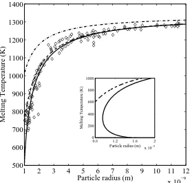
2.1 Size dependence of the melting temperature of gold nanoparticles. Solid line

represents Tm from (2.4), dashed line corresponds to (2.2) and dash-dotted

line to Pawlow model. Diamonds are experimental data from [8]. The subplot

showsTm from (2.2) and (2.4) for radius below 2 nm. . . 33

2.2 Sketch of the problem configuration. . . 34

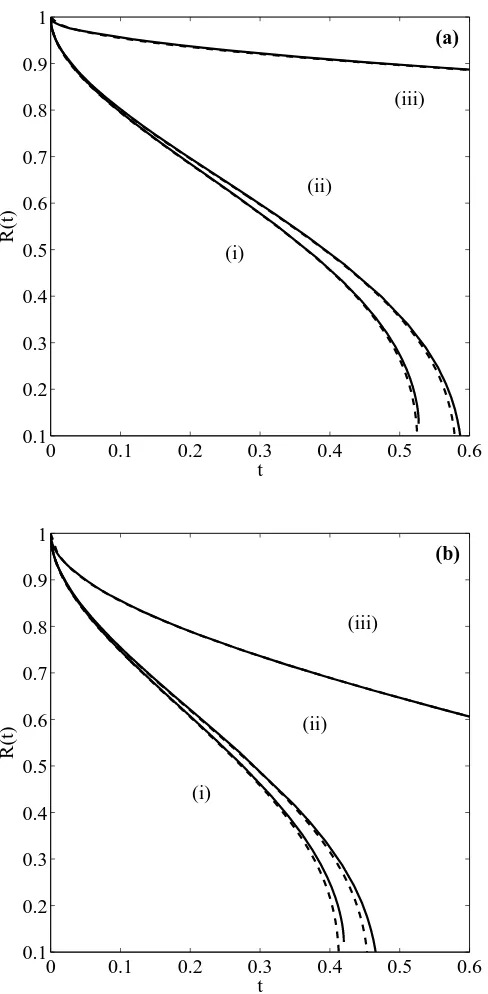
2.3 Position of the non–dimensional melting front R(t) for a nanoparticle with initial dimensional radius R0 = 10 nm, (a): β = 100 (b) β = 10. Curve (i) is

the solution of (2.23)–(2.24), (ii) the solution of (2.26) and (iii) the solution

of (2.27). . . 44

(16)

xvi LIST OF FIGURES

2.4 Position of the non–dimensional melting front R(t) for a nanoparticle with

initial radiusR0= 100 nm, (a): β = 100 (b)β = 10. Curve (i) is the solution

of (2.23)–(2.24), (ii) the solution of (2.26) and (iii) the solution of (2.27). . . 46

2.5 Comparison between one and two–phase solutions forβ = 100, (a)R0 = 10 nm

(b) R0 = 100 nm. . . 47

2.6 Blue is the solid phase, red the liquid phase and dashed the melting

temper-ature. For β= 100 and R0 = 10 nm. . . 49

3.1 Sketch of the model, showing a solid sphere of radius R(t) surrounded by a liquid layer with radiusRb(t). . . 58

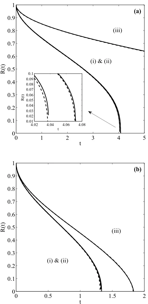
3.2 Evolution of the nondimensional melting frontR(t) for the two cases of study

ρ = 1.116 and ρ = 1, for β = 100 and R0 = 100 nm. Solid line represents

perturbation solution, dashed lines the numerical solution. . . 69

3.3 Dimensional temperature profiles for curves of Figure 3.2. The solid line

represents temperature for ρ = 1.116, the dashed lineρ = 1 and dotted line

shows the melt temperature variation. . . 69

3.4 Evolution of the nondimensional melting front R(t) for ρ= 1 andρ = 1.116,

forβ = 10 and R0 = 100 nm. . . 70

3.5 Evolution of the nondimensional melting front R(t) for ρ= 1.116 and ρ= 1,

for β = 100 and R0 = 10 nm. Solid line represents perturbation solution,

dashed lines the numerical solution. . . 71

3.6 Dimensional temperature profiles for curves of Figure 3.5. The solid line represents temperature for ρ = 1.116, the dashed lineρ = 1 and dotted line

shows the melt temperature variation. . . 72

3.7 Evolution of the nondimensional melting front R(t) for ρ= 1.116 and ρ= 1,

for β = 10 and R0 = 10 nm. Solid line represents perturbation solution,

dashed lines the numerical solution. . . 72

3.8 Relative importance of the termγR3

t againstρβRt forβ = 10, for

(17)

LIST OF FIGURES xvii

4.1 Representation of the solidification speed of copper (left) and salol (right) as

a function of the supercooling. The solid line represents the full expression

forst, the dashed line the linear approximation. . . 79

4.2 Linear kinetic undercooling with a) t _∈ [0,0.1], b) t _∈ [0,140]. The sets of

curves denote the numerical solution (solid line), HBIM (dashed) and small

and large time asymptotics (dash-dotted) results for the interface velocity

when β = 1. . . 101 4.3 Linear kinetic undercooling with t_∈[0,100] and a) β = 0.7, b) β= 1.5. The

sets of curves denote the numerical solution (solid line), HBIM (dashed) and

large time asymptotics (dash-dotted) results for the interface velocity. . . 102

4.4 Nonlinear kinetic undercooling with a)t_∈[0,0.1], b) t_∈[0,100]. The sets of

curves denote the numerical solution (solid line), HBIM (dashed) and small

time asymptotics (dash-dotted) results for the interface velocity when β= 1. 103

4.5 Nonlinear kinetic undercooling with a) β = 0.7, t _∈ [0,100] and b) β = 1.5,

t_∈[0,40] . The sets of curves denote the numerical (solid line) HBIM (dashed) and, whenβ = 0.7, asymptotic (dash-dot) solutions for the interface velocity. 104

4.6 Comparison of velocities and temperatures (at t= 1) predicted by the

non-linear (solid line), non-linear (dashed line) and Neumann (dot-dash) solutions for

β = 1.1. . . 105

5.1 Variation of s(t) for salol,k_≈1.4, c= 0.73 and (a)β = 0.7, (b)β = 1.3. . . . 119

5.2 Variation of s(t) for water,k_≈4, c_≈0.49 and (a)β = 0.7, (b)β = 1.3. . . . 120

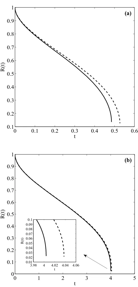
6.1 Evolution of the interfaceR(t) for the two-phase (solid line), largek(dashed),

small k (dash-dotted) and standard (dotted) formulations. Plot (a) corre-sponds ton= 2 (nanoparticle) and (b) ton= 1 (nanowire). . . 135

(18)

(19)

List of Tables

2.1 Approximate thermodynamical parameter values for water, gold, and lead.

The values for σsl are taken from [8, 48, 83]. . . 34

2.2 Melting times computed with the one–phase model. . . 48 2.3 Melting times computed with the two–phase model. . . 48

3.1 Approximate thermodynamical parameter values for gold. The value ofσsl is

taken from [8]. . . 62

3.2 Melting times for the caseρ= 1. Results for gold. . . 74

3.3 Melting times for the caseρ= 1.116. Results for gold. . . 74

4.1 Approximate thermodynamical parameter values for Cu and Salol, taken from

[4, 9, 24, 61]. . . 82

(20)

(21)

Chapter 1 Introduction

The phenomena of melting and solidification occurs in a multitude of natural and industrial

situations, from the melting of the polar ice caps or the solidification of lava from a volcano

to the manufacture of ice cream or the production of steel. For a material to undergo a solid-liquid phase change, thermal energy has to be delivered to the solid to break the bonds that

maintain its molecules or atoms in an organized lattice structure. For the opposite process,

energy must be taken from the liquid phase to slow down the motion of its molecules and

organize them back into a stable lattice structure. The mathematical formulation describing

this intuitively simple physical process is known as the Stefan problem, named after the

Slovene physicist Josef Stefan.

Scientific discoveries are being made every day that are changing the world we live in.

New observations and experiments lead to established scientific theories being revisited,

updated and possibly started from scratch. Following the philosophy of the pioneers of the

Stefan problem this thesis provides a mathematical description and analysis of new observed

physical phenomena, introducing appropriate modifications to classical phase change theory.

The mathematical models discussed in this thesis are linked with industrial processes on materials manufacturing and the working mechanisms of new technological applications. In

particular, we develop mathematical models describing the melting process of nanoparticles

and the solidification of supercooled liquids. In addition, more fundamental questions, for

(22)

2 CHAPTER 1. INTRODUCTION

example concerning the energy conservation of such systems, arose during the development

of the models and led to a revision of the standard formulation of Stefan problems.

Note, this thesis is built from five published papers, each of which contain an introduction

and literature survey. Consequently in this chapter we will not go into great detail on the

literature, all the relevant sources will be cited in the introduction section of each chapter.

In chapters 2 and 3 we present mathematical models describing the melting process of

nanoparticles. In these models the characteristic melting point depression of nanoparticles

is described by the Gibbs-Thomson relation. In chapter 2 we present a generalized version

of the Gibbs-Thomson relation that shows good agreement with experimental data down

to a few nanometers. Then, the relation is coupled with the heat equations for the solid

and liquid phase, and the Stefan condition. The standard perturbation method for large

Stefan number is utilized to reduce the system to a pair of easily solvable ordinary

differen-tial equations (ODE). We highlight the strong effect of the melting point depression when

compared to the equivalent classical Stefan problem solution. The solutions found show interesting features observed experimentally, such as the ultra-fast melting velocity as the

radius of the nanoparticle tends to zero. In chapter 3 the model studied in chapter 2 is

extended, allowing for the densities of the solid and liquid phases to take different values.

This seemingly inoffensive assumption leads to a remarkably different model formulation;

requiring an advection term in the heat equation for the liquid, an extra cubic term for the

velocity in the Stefan condition and a second moving boundary tracking the expansion of the

liquid phase. The solution methodology is analogous to that in chapter 2. The introduction

of the density jump between phases has a profound effect on the solution, showing more than a 50% difference in the melting times with the equivalent model assuming equal densities.

In chapter 4 we study the solidification process of a supercooled liquid. Again the phase

change temperature is variable but now it is related to the reduced mobility of the supercooled

liquid molecules. The interface temperature, which is lower than the ideal freezing point, depends nonlinearly on the velocity of the solidification front. Previous studies have focused

on the standard problem with a constant phase change temperature or on the case of very

(23)

3

phase change temperature is approximately linear. We analyse the problem in three possible

scenarios; with the full nonlinear relation, the linearized approximation and the standard

case, with constant interface temperature. Asymptotic solutions for small and large times

are provided and compared with numerical and approximate solutions by the Heat Balance

Integral Method. The introduction of the characteristic nonlinear behaviour of the phase

change temperature shows the unsuitability of the classical Neumann solution to describe

the solidification of supercooled melts.

In general, finding a solution to the Stefan problem requires solving heat equations for

the solid and liquid phases subject to a condition in the solid-liquid interface describing the

evolution of the phase change front. Sometimes, it is convenient to reduce the problem by

assuming the solid or the liquid to be at the phase change temperature and only solve the

heat equation for the remaining phase. This simplified model is commonly referred to as the one-phase Stefan problem. In chapters 2, 3 and 4 we propose models where the phase

change temperature varies, meaning that a truly one-phase problem will never exist (since

the melting or freezing temperature is a function of time). Hence, the one-phase reduction

based on assuming one of the phases at the constant phase change temperature does not

hold. This leads us to look for consistent ways to formulate the one-phase Stefan problem for

cases where the phase change temperature is variable. In chapter 5 we specifically deal with

the derivation of an accurate one-phase reduction of the Stefan problem for the solidification

of supercooled melts. Previous formulations of the one-phase reduction have appeared not

to conserve energy or relied on non-physical assumptions. In chapter 5, we derive an energy conserving formulation for the one-phase supercooled Stefan problem. Numerical solutions

for the proposed one-phase model are tested against solutions for the full two-phase problem.

The results show excellent agreement and improve considerably on the accuracy of previous

one-phase formulations.

The study of the one-phase reduction of the Stefan problem with linear supercooling carried out in chapter 5 opens the door to tackle the problem from a more general point

of view. With the advent of new technologies, phase change processes where solid-liquid

(24)

frequent. This serves as the motivation for chapter 6 where the derivation of the one-phase

reduction of the Stefan problem is examined in detail via energy arguments. A general

one-phase model of the Stefan problem with a generic variable one-phase change temperature, valid

for spherical, cylindrical and planar geometries, is provided. Finally, the model is solved

numerically for the case where the phase change temperature depends on the inverse of the

melting front (which is related to the melting process of nanoparticles studied in chapters 2

and 3). As in chapter 5 the results are compared to the two-phase model and show excellent accuracy.

In the following section of this introduction we briefly describe the historical roots of

the Stefan problem. In the second section we introduce the formulation of the problem and

summarize some of the standard analytical techniques used to tackle Stefan problems. Then,

we present the extensions that have to be introduced to the standard problem to account

for the variable phase change temperature of nanoparticles and supercooled liquids, and the

appropriate way to formulate the one-phase Stefan problem for such situations.

1.1 Historical roots of the Stefan problem

The Stefan problem, named after the Slovene physicist Joˇzef Stefan (1835-1893), is a particu-lar kind of moving boundary value problem that originally aimed to describe the solid-liquid

phase change process [53, 94, 107, 117]. Stefan problems, are characterized by having a

boundary of the domain which is moving and, therefore, its position is unknown “a priori”.

The position of the moving boundary is a function of time (and sometimes space) and must

be determined as part of the solution. The differential equations in a Stefan problem are

generally, but not restricted to, of parabolic type. The most common example of a

Ste-fan problem is that describing the ice-water phase transition. This requires solving heat

equations for the ice and water phases, while the position of the front separating the two states, the moving boundary, is determined from an energy balance, referred to as the Stefan

condition.

Stefan carried out extensive analytical and experimental work on physical situations

(25)

reac-1.1. HISTORICAL ROOTS OF THE STEFAN PROBLEM 5

tions [101] and liquid-vapor phase change [100, 103, 106]. Indeed, his most popular and cited

work in the field is [107] (a reprinted version of [102] for the journal Annalen der Physics

und Chemie) where he studied ice formation in the polar Arctic seas. His model described the seawater initially at the freezing temperature and the air in contact with the water to

be at a constant temperature below the freezing point, thus, triggering ice formation at the

air-water interface [115]. The resulting growing ice layer was found to be proportional to the

square root of time. However, Stefan’s major contribution to science was the experimental finding that states the thermal energy radiated by an object is proportional to the fourth

power of its temperature, the law of Stefan-Boltzmann. The second name is due to the

Aus-trian physicist Ludwig Boltzmann (1844-1906), Stefan’s pupil, who derived the relationship

from first principles. Above all, Stefan was a brilliant experimentalist who is also known for

being the first to accurately measure the thermal conductivity of gases [17].

Although Stefan carried out wide ranging research concerning phase change, from

exper-imental to theoretical work, and the Stefan problem was named after him, he was not the

first to formalize and solve the problem. In the 18th century, the Scottish medical doctor Joseph Black (1728-1799) introduced for the first time the concept of latent heat, a key

in-gredient to understanding the physical mechanism of phase change. Later on, Jean Baptiste Joseph Fourier (1768-1830), a French mathematician and physicist, provided the necessary

physics and mathematics to the theory of heat conduction. In the 19th_{century, the physicist}

Gabriel Lam´e (1795-1850) and the mechanical engineer Emile Clapeyron (1799-1864) were

the first to mathematically couple the concept of latent heat with the heat conduction

equa-tion, whilst extending Fourier’s work on the estimate of the time elapsed since the Earth

began to solidify from its initial molten state [53, 94]. They initially assumed the Earth to

be in a liquid phase at the melting temperature (a one-phase problem). Due to an abrupt

temperature drop at the surface the freezing process was initiated. They found the solid

crust to grow proportional to the square root of time (just as Stefan later found in his work [102, 107]). Unlike Stefan, Lam´e and Clapeyron did not determine the value of the constant

of proportionality. In a series of lectures in the early 1860s, Franz Ernst Neumann

(26)

of Lam´e and Clapeyron [53], with the initial temperature above the melting point [17, 94]

(so dealing with a two-phase problem). However, his work was not published until 1901 by

Heinrich Weber in [117]. Today, the solution to the classical Stefan problem receives the

name of Neumann solution in honor of the German scientist.

The motivation of the Stefan problem was the need to mathematically formulate and

describe observed natural physical phenomena, such as the melting, solidification or

evapo-ration of a substance. Nowadays, it is well known that Stefan problems arise in numerous industrial and technological applications, such as the manufacture of steel, ablation of heat

shields, contact melting in thermal storage systems, ice accretion on aircraft, evaporation

of water, and a long etcetera [3, 16, 27, 40, 43, 108]. The fact that the Stefan problem has

been studied and applied in a wide variety of situations is evident by simply looking at the

review on the subject from 1988 [108], where around 2500 references were given. Over 20

years later, the number of references has exponentially increased. A quick search in Google

Scholar gives around 422K references in the period 1999-2014. Hence, it is clearly impossible

to establish here a complete list of references of papers on the subject. However, there are

some reference books on Stefan problems and its applications that have been particularly important for the elaboration of this thesis that the interested reader may wish to consult

[3, 16, 19, 38, 40].

1.2 Formulation and standard mathematical techniques

The Stefan problem is a mathematical model describing the process of a material undergoing a phase change. The mathematical formulation of the problem involves heat equations for

the solid and liquid phases and a condition at the solid-liquid interface, the Stefan condition,

that describes the position of the phase change front. At the moving phase change boundary,

x=s(t), the temperature is fixed at the constant bulk phase change temperature,T∗ m. The

most basic form of Stefan problem arises when considering the melting of a semi-infinite,

one-dimensional slab occupying x_≥0, where the phase change is driven by a heat source at

(27)

1.2. FORMULATION AND STANDARD MATHEMATICAL TECHNIQUES 7

TH

x= 0

Liquid Solid

T∗ m

[image:27.595.141.440.102.183.2]

x=s(t)

Figure 1.1: Semi-infinite slab melting fromx = 0 due to the high temperatureTH. Dashed

line depicts the liquid-solid interface,s(t), and the arrow the direction of motion of the phase change front.

The governing equations of the model are

clρl ∂T

∂t = kl ∂2_T

∂x2 on 0< x < s(t) , (1.1)

csρs ∂θ

∂t = ks ∂2_θ

∂x2 on s(t)< x <∞ , (1.2)

where T represents the temperature in the liquid, θ the temperature in the solid, s= s(t)

the position of the moving boundary,kthe thermal conductivity,ρthe density,cthe specific

heat and subscriptssandlindicate solid and liquid, respectively. The position of the moving fronts(t) is determined by the Stefan condition

ρlLm ds dt =ks

∂θ ∂x−kl

∂T

∂x on x=s(t), (1.3)

whereLm is the latent heat. At the interfacex=s(t) we haveT(s, t) =θ(s(t), t) =Tm∗ and,

defining the heat source driving the melting as a constant temperatureTH > Tm∗, atx = 0

we haveT(0, t) =TH. Obviously, att= 0 the liquid phase does not exist, sos(0) = 0. From

a formal point of view we still need to define a boundary and an initial condition forθ but

for the following argument this is unnecessary.

A very common simplification of the Stefan problem consists of assuming one of the

phases to be initially at the phase change temperature [40]. This removes one of the two heat equations and provides a simpler form of the Stefan condition by eliminating one of

the temperature gradients. In this way, one of the two phases is effectively omitted and the

(28)

the solid region initially at the melting temperature in the system (1.1)-(1.3) the problem

reduces to

clρl ∂T

∂t = kl ∂2T

∂x2 on 0< x < s(t) , (1.4)

T(0, t) = TH , (1.5)

T(s, t) = T∗

m , (1.6)

ρlLmds

dt = −kl ∂T

∂x on x=s(t). (1.7)

Only one practically useful exact solution exists for problems of the form (1.4)-(1.7), which is expressed in terms of the error function [38, 40, 53, 107]. Several analytical,

ap-proximate and numerical methods have been employed in the past to analyse Stefan problems

when no analytical solution exists [3, 10, 40, 43, 55, 64, 66, 113]. In this thesis we mainly

focus on analytical and approximate techniques. Numerical solutions are generally provided

to verify approximate solutions. Now, we provide a quick overview of some standard

math-ematical techniques for Stefan problems that will be used later in this thesis.

1.2.1 Similarity variables

The order of a partial differential equation can often be reduced by rewriting the equation in

terms of a similarity variable, grouping in the new variable two or several former independent

variables, and thus reducing the order of the equation. For instance, if we have a partial

differential equation whose independent variables are x and t we may look for a similarity

variable of the form ξ=c tνxγ [16, 40]. Assuming the nondimensional version of (1.4)–(1.7)

∂T ∂t =

∂2T

∂x2 on 0< x < s(t) , (1.8)

T(0, t) = 1, (1.9)

T(s, t) = 0, (1.10)

βds

dt = − ∂T

(29)

whereβ =L/c(TH −Tm∗) is the Stefan number, and applying the similarity transformation

ξ=x/√tto (1.8), the PDE is reduced to

Fξξ=− ξ

2Fξ , (1.12)

whereF(ξ) =T(x, t). This has the general solution

F(ξ) =C1+C2erf

ξ

2

. (1.13)

This may be solved in terms of the error function. Imposing the boundary conditions and

rewritting in terms of the original variables, the solution to the problem (1.8)–(1.11) is

T(x, t) = 1₋

erf x

2√t

erf(λ) , s(t) = 2λ √

t , (1.14)

where the constant λis the solution of

β√πλeλ2 erf(λ) = 1. (1.15)

Expressions (1.14)-(1.15) receive the name of Neumann solution.

Although similarity transformations can only provide exact solutions to a very small

num-ber of Stefan problems, they represent the basis for analytical progress to other formulations

when combined with other techniques such as perturbation methods, as in chapter 4.

1.2.2 Boundary–fixing transformations

Another useful tool to simplify problems like (1.4)–(1.7) is the boundary–fixing

transfor-mation [16, 41, 40]. This is of particular interest when looking for numerical solutions,

where working with a moving boundary is always troublesome. For example, the boundary

immobilising coordinate η=x/s(t) applied to (1.4)–(1.7) yields

∂F2 ∂η2 =s

2∂F

∂t −ηs ds dt

∂F

(30)

and boundary conditions

F(0, t) = 1 , F(1, t) = 0, βsds dt = −

∂F ∂η η=1 , (1.17)

where F(η, t) = T(x, t). This fixes the problem of a moving domain, since the original

domain x _∈ [0, s(t)] is now mapped on to η _∈ [0,1]. However, with the standard Stefan

problem we find s _∼ √t and so st ∼ 1/√t (which appears in (1.16)) is singular at t = 0.

This difficulty may be removed by working in terms ofz=s2, so

∂F2

∂η2 =z

∂F ∂t − η 2 dz dt ∂F ∂η , β 2 dz dt =−

∂F ∂η η=1 . (1.18)

In this form the equations are amenable to standard finite difference techniques.

The variable η = x/s(t) transforms the domain [0, s(t)] into [0,1]. However, the

one-phase reduction of the Stefan problem can be such that the heat equation lies in the region

s(t)< x <_∞ instead of 0< x < s(t). If this is the case, then the boundary fixing variable

that we use is η = x₋s(t), which transforms the domain from [s(t),_∞] into [0,_∞]. In

the case of solving the two-phase problem we could use both transformations, one for each

phase, i.e., η1 = x/s(t) and η2 = x−s(t). Indeed, other transformations arise depending

on the nature of each problem, as in chapters 2 and 3 where the geometry of the domain is

spherical.

1.2.3 Perturbation method

The aim of this method is to find an approximate solution to a problem, which cannot be

solved analytically, by means of a power series solution in terms of a small parameter [42].

For instance, we will now describe what is known as the large Stefan number expansion,

see [40]. Consider the problem (1.8)–(1.11). For large values of β we can define the small

parameterǫ= 1/β _≪1 and the Stefan condition may be written as

ds dt =−ǫ

∂T ∂x

x=s

(31)

From (1.19) we see that at leading order st = 0 and, after applying the initial condition,

s= 0, meaning that the front is approximately stationary. This indicates that a large Stefan

number corresponds to slow melting (as can be seen from β _∝ 1/(TH −Tm∗), so large β

implies small heating). In order for the front to move (at leading order) we need to rescale

timet=τ /ǫ. This leads to

ǫ∂T ∂τ =

∂2_T

∂x2 ,

ds dτ =−

∂T ∂x

x=s

. (1.20)

Hence, we try the expansion

T =T0+ǫT1+ǫ2T2+. . . , (1.21)

and find

O(ǫ0) : 0 =∂

2_T 0

∂x2 → T0 = 1−

x

s (1.22)

O(ǫ1) : ∂T0

∂τ = ∂2T1

∂x2 → T1 =

sτ

6

x3 s2 −x

(1.23)

O(ǫ2) : ∂T1

∂τ = ∂2_T

2

∂x2 . . . (1.24)

If we substitute these solutions into the Stefan condition we find

ds dτ =−

−1

s+ǫ

1 3 ds dτ , (1.25) which gives s= r 6τ

3 +ǫ =

√

2τ1₋ ǫ 6+. . .

(32)

0.0 0.5 1.0 1.5 2.0 2.5 3.0 x

0.0 0.2 0.4 0.6 0.8 1.0

T

(x

,t

)

0 2 4 6 8 10

t 0.0

0.5 1.0 1.5 2.0 2.5 3.0 3.5

s(

[image:32.595.98.491.107.291.2]

t)

Figure 1.2: Exact (solid), leading order perturbation (dotted) and first order perturbation (dashed) solution for the one-phase Stefan problem (1.8)-(1.11) forβ = 2. Left: temperature of the liquid at t= 10. Right: evolution of the melting front.

In figure 1.2 we compare the exact solution, the leading order perturbation solution and

the perturbation solution to _O(ǫ) . We observe that the correction introduced by the _O(ǫ)

term from (1.23) has a strong effect, and even for the relatively large value of the small

parameter used,ǫ= 0.5, the solution converges very quickly to the exact solution.

We note that after the _O(ǫ) solution, equation (1.23), we cannot take the perturbation

solution further. We stopped the series inT2 since it depends on ∂T_∂τ1 and so involves a term

sτ τ. Since we only have a single initial condition we cannot deal with this extra term that

makes the Stefan condition second order in time. We may overcome this problem by defining

the boundary–fixing transformation η = x/s and a new time variable τ(t) = s(t), so that

T(x, t) =F(η, τ) [40]. Then the problem (1.8)–(1.11) becomes

Fηη =τ τt(τ Fτ −ηFη), βτ τt= −Fη|_η₌₁, F(0, τ) = 1, F(1, τ) = 0 , (1.27)

and for a large Stefan number we have

(33)

Since (1.27a) containsτ τtwe substitute (1.28) into it and perform the following expansion

F(η, τ) =F0+ǫF1+ǫ2F2+. . . , (1.29)

to give

O(ǫ0) : 0 =∂

2_F 0

∂η2 → F0= 1−η (1.30)

O(ǫ1) : ₋C(τ) (τ F0τ −ηF0η) = ∂2F1

∂η2 → F1=

C(τ) 6 1−η

2

η (1.31)

O(ǫ2) : ₋C(τ) (τ F1τ −ηF1η) = ∂2F2

∂η2 → . . . , (1.32)

whereC(τ) = Fη|_η₌₁. An important point is that we could take this expansion as far as we

like as there is no issue with derivatives ofτ, and the only reason to stop is that the algebra

becomes tedious. Once, we have enough terms in the expansion we replace F in the Stefan

condition and solve the equation for τ.

1.2.4 The Heat Balance Integral Method

The heat balance integral method (HBIM) introduced by Goodman [32] is a well-known

approximate method for solving Stefan problems [3, 10, 64, 73, 71]. The basic idea behind the method is to approximate the temperature profile, usually with a polynomial, over some

distance δ(t) known as the heat penetration depth. This is a fictitious measure of the point

where the thermal boundary layer ends. The heat equation is then integrated to determine

a ordinary differential equation for δ(t). The solution of this equation, coupled with the

Stefan condition then determines the temperature and position s(t). In chapter 4 we apply

the HBIM to a one-phase Stefan problem related to the solidification of a supercooled melt.

We will now use this physical situation to illustrate the HBIM.

Consider the solidification of a supercooled liquid which initially occupies the semi-infinite

(34)

one-phase Stefan problem describing this situation may be written as

∂T ∂t =

∂2T

∂x2 on s < x <∞ , (1.33)

T(s, t) = 0, T(_∞, t) =₋1, T(x,0) =₋1 , (1.34)

where T represents the temperature of the supercooled liquid, the temperatureT = 0

rep-resents the freezing temperature and T =₋1 is the far field and initial temperature of the

liquid. The Stefan and the initial condition at the solidification fronts(t) are

βds dt =−

∂T ∂x

x=s

, s(0) = 0 . (1.35)

The system (1.33)-(1.35) can be solved analytically by means, for instance, of similarity variables and has the exact solution

T =₋1 +erfc x/2 √

t

erfc(λ) , s= 2λ √

t , (1.36)

where the value ofλis obtained by solving the transcendental equation

β√πλ erfc(λ)eλ2 = 1 . (1.37)

The solution (1.36)-(1.37) represents the particular form of the classical Neumann solution

for the one-phase supercooled Stefan problem (1.33)-(1.35).

The first step when using the HBIM consists in defining the heat penetration depth δ(t),

the point after which we consider the temperature gradient to be negligible. In our model,

x = δ(t) represents the point where the temperature of the liquid is sufficiently close to

the far field temperature T = ₋1. Note, this means we work over the domain [s(t), δ(t)].

The second step consists in assuming a temperature profile describing the thermal response of the material. This involves typically polynomials, although logarithmic, exponential and

error functions have been also utilized in the literature [15, 65, 69]. The profile will include

(35)

current problem, we propose

T(x, t) =a1+a2

δ₋x δ₋s

+a3

δ₋x δ₋s

n

. (1.38)

The final step, is the integration of the heat equation over the spatial variablex to produce

the heat balance integral.

In summary, using the HBIM, the problem (1.33)–(1.34) translates into

Z δ

s ∂T

∂t dx=

Z δ

s(t)

∂2T

∂x2 dx on s < x < δ , (1.39)

T(s, t) = 0, T(δ, t) =₋1, Tx(δ, t) = 0 . (1.40)

It is straightforward to see that the parameters a1, a2 and a3 from the assumed profile

(1.38) are readily found from the boundary conditions (1.40). Hence, the temperature profile

becomes

T(x, t) =₋1 +

δ₋x δ₋s

n

. (1.41)

Equation (1.39) may be rearranged by means of the Leibniz integral rule to give

d dt

Z δ

s

Tdx₋T

x=δδt+T

x=sst=Tx

x=δ−Tx

x=s . (1.42)

Then, assuming the polynomial to be quadratic, n= 2, and replacing (1.41) into (8.6) and

(1.35) results in two ordinary differential equations

dδ

dt = (3β−2) ds

dt, δ(0) = 0, (1.43)

ds dt =

2

β(δ₋s), s(0) = 0, (1.44)

with solutions

δ = (3β₋2)s, s= s

4t

2β(β₋1) . (1.45)

Substituting the expressions (1.45) in (1.41) the temperature profile is completely

(36)

0 1 2 3 4 5 6

x −1.0

−0.8 −0.6 −0.4 −0.2 0.0

T

(x

,t

)

0.0 0.2 0.4 0.6 0.8 1.0

t 0.0

0.2 0.4 0.6 0.8 1.0

s(

t)

Figure 1.3: Exact (solid) and HBIM (dashed) solution for the one-phase supercooled Stefan problem for β = 2. Left: temperature of the liquid at t= 1. Right: time evolution of the solidification front.

The main advantage of the HBIM is that it reduces a difficult problem such as (1.33)–

(1.35) into a pair of easily solvable ODEs. In this case it may not seem of great use, since an exact solution exists, but for more complex problems such as the ones developed in this thesis,

the HBIM is sometimes of incalculable help. In figure 1.3 we compare the exact solution

(1.36) and the HBIM solution withn= 2. It is clear that even forn= 2, the simplest realistic

choice, the HBIM captures satisfactorily the behaviour of the exact solution. However, we

note that even though Goodman’s original choice was n= 2 the method may be improved

by assuming n as an unknown in the problem and determining it as part of the solution.

One option, known as the Optimal HBIM [70, 71], consists in choosing an exponentn that

minimizes the least squares error

En= Z δ

s

f(x, t)2dx where f(x, t) = ∂T

∂t − ∂2T

∂x2. (1.46)

This method significantly improves the accuracy of the HBIM and provides an error measure that does not require knowledge of an exact or numerical solution. For certain problems,

for example when the boundary conditions are time–dependent, n may vary with time.

(37)

1.3. EXTENSIONS TO THE STANDARD PROBLEM 17

largest value of En usually occurs. Other extensions of the HBIM based on determining n

as part of the solution exist. This is the case of the Refined Integral Method (RIM) [64, 91],

that integrates the heat equation twice to obtain an extra equation forn, or the Combined

Integral Method [65, 73], a combination of the Optimal HBIM and the RIM.

1.3 Extensions to the standard problem

To understand phase change in a more general situation several modifications must be

intro-duced in the formulation of the standard Stefan problem, for example to include phenomena such as the melting point depression of nanoparticles, the velocity dependent freezing

temper-ature in supercooled liquids or the expansion upon melting of the liquid phase of a material.

Such modifications require us to review the derivation of the governing equations of the

Stefan problem, so, we briefly describe how to derive the heat equation from the energy

conservation equation and the Stefan condition from an energy balance at the solid-liquid

interface. This will provide general mathematical expressions that will be easily adapted for

modeling each physical problem dealt with within this thesis.

Bird, Stewart and Lightfoot [7] write down an energy balance, stating that the gain

of energy per unit volume equals the energy input by convection and conduction and the

work done by gravity, pressure and viscous forces. Assuming the effects of gravity, viscous

dissipation and pressure are negligible an appropriately simplified version of their energy

conservation equation is

∂ ∂t

ρ

I+v

2

=_{−∇ ·}

ρv

I+v

2

+q

, (1.47)

where ρ is the density,I the internal energy per unit mass, vthe velocity, v=_|v_|, and the

conductive heat flux q =₋k_∇T. The quadratic term in the velocity is the kinetic energy component. The internal energy is defined by

I =cl(T−Tm∗) +Lm in the liquid, (1.48)

(38)

where T represents the temperature in the liquid and θ that in the solid. Again neglecting

the work done by gravity, pressure and viscosity conservation of mechanical energy for a

flowing liquid is

∂ ∂t

1 2ρlv

2

=_{−∇ ·}

1 2ρlv

2_v

. (1.50)

Noting that

∇ ·(ρIv) =v_{· ∇}(ρI) +ρI_{∇ ·}v=v_{· ∇}(ρI) , (1.51)

for an incompressible fluid, then equations (1.47) and (1.50) may be combined to give

∂

∂t[ρI] =−∇ ·[ρvI +q] =−v· ∇(ρI)− ∇ ·q. (1.52)

All versions of the heat equation analysed in the thesis can be deduced from expression

(1.52). For example, in the one-dimensional case, _∇ = ∂/∂x, substituting (1.48)-(1.49) in

(1.52) and assuming that none of the phases is moving, v= 0, yields (1.1)-(1.2), the most

basic form of the heat equation for the Stefan problem.

By means of (1.47) we have specified energy conservation in the solid and liquid phases.

The study of the energy conservation across the solid-liquid interface will lead to the Stefan

condition. To examine the energy conservation at the phase change boundary,s(t), requires

the Rankine-Hugoniot condition

∂f

∂t +∇ ·g= 0 ⇒ [f]

+

−st= [g·n]

+

− , (1.53)

where n is the unit normal and f, g are functions evaluated on either side of s(t) [3] (for

a derivation of (1.53) in the one-dimensional case, see Appendix). Applying (1.53) to the energy balance (1.47) in the one-dimensional case, where

f =ρ

I+v

2

, g_·n=ρv

I+ v

2

(39)

andq =₋ks∂θ/∂xorq=−kl∂T /∂x(for solid and liquid, respectively), and assuming that

the solid is stationary, gives the Stefan condition

ρl

cl(T(s, t)−Tm∗) +Lm+ v2

2

−ρscs(θ(s, t)−Tm∗)

st

=ρlv

cl(T(s, t)−Tm∗) +Lm + v2

2

−kl ∂T ∂x

x=s(t)

+ks ∂θ ∂x

x=s(t)

.

(1.55)

Equivalent to (1.52) for the heat equations, equation (1.55) serves as starting point to obtain

all the Stefan conditions used throughout the thesis. For example, if the liquid does not move

(v= 0) and the temperature ats(t) is the bulk phase change temperature,T(s, t) =θ(s, t) =

T∗

m, then the standard form of the Stefan condition, (1.3), is retrieved.

In the following sections we will use (1.52) and (1.55) to obtain heat equations and Stefan

conditions that will be used later in subsequent chapters. In section 1.3.1 we introduce

the specific form of the Stefan condition for cases where the interface temperature differs

from the standard phase change temperature. Then, we specify the particular expressions

describing the interface temperature for the phase change processes of nanoparticles and

supercooled melts. In section 1.3.2 we present the changes in the governing equations and

boundary conditions induced by considering a density jump between the solid and liquid

phases. Finally, in section 1.3.3 we discuss the effect of a variable phase change temperature

when reducing the two-phase Stefan problem to a one-phase problem. In addition, we show how to derive an accurate one-phase model based on consistent physical assumptions.

1.3.1 Variable phase change temperature

There are many practical situations where the phase change temperature cannot be

consid-ered constant, e.g. when the phase change occurs in the presence of a curved interface or in supercooled conditions [3, 4, 19, 38]. In both cases the interface temperature is a function of

time. With the standard Stefan problem,T(s(t), t) =θ(s(t), t) =T∗

m, whereTm∗ is the bulk

(40)

is replaced by

T(s(t), t) =θ(s(t), t) =TI(t) , (1.56)

where the form ofTI(t) will depend on the physical problem. Substituting (1.56) in (1.55),

assuming the liquid is stationary and phases with the same density, the Stefan condition becomes

ρl[Lm−(cl−cs)(Tm∗ −TI)]st=ks ∂θ ∂x−kl

∂T

∂x on x=s(t). (1.57)

The difference between (1.57) and the standard Stefan condition (1.3) is the term (cl −

cs)(Tm∗ −TI). Inspection of (1.57) reveals that, ifTI =Tm∗ the standard form is retrieved.

One way to reduce (1.57) to its standard form, but keeping (1.56) in the model, is by assuming

the specific heat for the liquid and solid phase are equal, i.e. cl =cs. However, as shown in

chapter 2, in the context of nanoparticle melting, this assumption leads to inaccurate results.

In the two subsequent sections, we introduce the concept of a nanoparticle and

pro-vide motivation for the study of its phase change process. We present the Gibbs-Thomson equation, the mathematical expression for TI describing the melting point depression of

nanoparticles. Then, we discuss supercooled liquids and the interest in their solidification

process. Further, we provide a nonlinear expression for TI modeling the dynamics of the

molecules at the solid-liquid interface.

Nanoparticles

According to the International Union for Pure and Applied Chemistry, a nanoparticle is a

particle of any shape with dimensions in the range 10−9_-10−7_{m [110]. Nanoparticles have} fascinated the scientific community since the second half of the last century, due to their

remarkable physical properties, which are not obseerved at the bulk scale [35, 36, 87]. Despite

the reduced size of nanoparticles, continuum theory describing phase change processes is considered to be valid for particles with radii larger than 2 nm [36]. Kofman et al[48] state that at scales smaller than 5 nm the melting process is discontinuous and dominated by

(41)

study of nanoparticle melting between 2-5 nm.

From a practical point of view, nanoparticles are very interesting because they are

cur-rently being used for new and revolutionary technological applications such as phase change

memories [22, 99], phase change materials [46], nanofluids [116] and in biological applications

such as drug carriers [6, 31, 57, 88] or thermal agents for hyperthemia treatments of tumours

[44]. Some of the aforementioned applications work directly in the phase change regime or

occur at very high temperatures, indicating the importance of understanding the thermal

response and likely phase change behaviour of nanoparticles.

An interesting property directly affecting the melting process of nanoparticles is the

melting point depression or Gibbs-Thomson effect [3, 8, 18, 98], which is a well-known

physical phenomena that occurs on surfaces with a high curvature. A nanoparticle can be

imagined as a cluster of atoms. The surface atoms are more weakly bound to the cluster

than the bulk atoms and melting proceeds by exciting the surface atoms and separating them from the bulk. For a sufficiently large cluster the energy required is relatively constant since

each surface atom is affected by the same quantity of bulk atoms. However, as the cluster

decreases in size the surface atoms are surrounded by an inferior number of bulk atoms and,

so feel less attraction to the bulk. Consequently, less energy is required for separation. This

translates into a decrease of the melting temperature at the surface of nanoparticles. The

most general form of the Gibbs-Thomson equation is given by

1

ρl −

1

ρs

(pl−pa) =Lm TI T∗ m − 1

+ (cl−cs)

TIln

TI T∗ m

+T∗

m−TI

+2σslκ

ρs

, (1.58)

where ρ is the density, Lm the latent heat, c the specific heat, p the pressure and σ the

surface tension [3]. The subscripts sandl indicate solid and liquid, respectively. The mean

curvatureκ is given by

κ= 1 2 1 R1 + 1 R2 , (1.59)

where R1 and R2 are the two principal radii of curvature. If R is the radius of a sphere or

cylinder, thenκ= 1/Rorκ= 1/2R, respectively.

(42)

described by (1.58), is analysed. Pressure differences are not considered and thus the left

hand side of (1.58) is set to zero. In the presence of a high curvature, as on the nanoparticle

surface, even if the pressure variation is relatively high, the term is small compared to the

rest, as will be discussed in chapter 2. Under the assumption that the specific heat remains

constant throughout the liquid and solid phase (cl=cs), expression (1.58) yields the classical

form of the Gibbs-Thomson relation

TI =Tm∗

1₋2σslκ

ρsLm

. (1.60)

In chapter 3 we study the effect of a density change between the solid and liquid phase in the nanoparticle melting process. In this case, to obtain a more tractable mathematical model

we consider cl=cs and use (1.60) instead of (1.58).

In chapters 2 and 3 we consider models with a spherical geometry. In these models,

melting begins due to a high temperature at the surface of the nanoparticle. As the liquid

phase grows at the nanoparticle surface, the solid phase is reduced in turn. The

solid-liquid interface, which also defines the radius of the solid portion, is denoted by R =R(t).

As melting proceeds the curvature of the interface R(t) increases rapidly. Therefore, the

melting point depression due to the Gibbs-Thomson effect at R(t) is larger as the process

continues leading to a remarkable increase in the velocity of the nanoparticle melting process.

High curvature induces a variable phase change temperature on the surface. In

super-cooling conditions the molecular attaching mode at the solid-liquid interface plays a role and

leads to a decrease of the phase change temperature, which we now introduce.

Supercooled melts

Supercooling is the action of cooling down a liquid below its standard freezing point. These

liquids are trapped in a metastable state and are ready to solidify as soon as the opportunity arises. The supercooled state of a liquid can be achieved, for instance, by applying very high

cooling rates, cooling down a liquid adjacent to a material surface with a particular molecular

(43)

at high altitude are a good example of this as they contain tiny droplets of water that in

the absence of seed crystals do not form ice despite the low temperatures. Freezing rain

is caused by the precipitation of these drops that, upon impact with any surface, instantly

freeze, and sometimes accumulate to a thickness of several centimeters. In fact, when an

aircraft flies through a cloud of supercooled droplets it provides a large nucleation site. As a

consequence there can be significant ice accretion, which can have a detrimental effect on the

plane’s performance [72]. However, materials formed from supercooled melts have desirable properties for many technological applications, such as metallic glass [109]. The interest in

these kind of materials lies in the fact that they lack a crystalline structure, which provides

them with increased strength, durability and elasticity [109]. Furthermore, phase change

techniques in supercooled conditions are also being examined for the cryopreservation of

human ovarian cortex tissues and food storage [54, 68].

As a liquid is cooled down below its freezing point, the energy of the molecules and hence

their motion is decreased. As the solidification of a supercooled liquid begins the reduced

molecular motion in the liquid phase affects the ability of the molecules to move onto the

solid interface [4, 19]. In this situation the temperature at which the liquid solidifies is not

constant and depends on the velocity of the solidification front,st. The relationship between

the velocity and the temperature at the solid-liquid interface,TI, is given by

st= d∆h

6hT∗ m

e− q kTI₍_T∗

m−TI) , (1.61)

where d is the molecular diameter, h Planck’s constant, q the activation energy and k

the Boltzmann constant [4]. The parameter ∆h is the product of the latent heat and the molecular weight divided by Avogadro’s number. If the degree of supercooling, (T∗

m−TI),

is small (1.61) can be approximated in the linear form

TI(t) =Tm∗ −φst , (1.62)

whereφ= 6hTme q

kTm/(d∆h). We note that (1.61), as with the generalized Gibbs-Thomson

(44)

in combination with the heat equations and the Stefan condition. The role of the linear

approximation (1.62) in the Stefan problem is the same as that of the classical

Gibbs-Thomson relation (1.60); they can be directly incorporated as time-dependent boundary

conditions in the model.

In chapter 4 we study the solidification of supercooled melts by introducing (1.61) into the

one-phase Stefan problem. In previous studies of the supercooled Stefan problem the linear

approximation (1.62) has been used extensively, regardless of the degree of supercooling.

Hence, we analyse the problem with the linear approximation and we test its performance

against the solution using the nonlinear form (1.61). In addition, we show how the Neumann

solution (1.36) remarkably overestimates the velocity of propagation of the freezing front in

contrast with the solutions obtained using (1.61) and (1.62).

1.3.2 The effect of density change

One of the basic assumptions in standard analyses of Stefan problems is that of constant

density,ρl=ρs. However, in reality, melting and solidification processes are always affected

by changes in the density, which translate physically to the shrinkage or expansion of one

of the phases. For instance, in countries with cold climates, pipe bursting is a recurrent problem. As water freezes, the molecules crystallize into a hexagonal form, which takes up

more space than molecules in the liquid form, thus, causing the pipe to burst.

The changes in the mathematical model when the density jump between phases is

intro-duced are significant. To demonstrate this we will now focus on the case where the liquid phase moves due to expansion upon melting. Then, expression (1.52) combined with (1.48)

and the heat flux q=₋kl∇T, yields the heat equation

ρlcl

∂T

∂t +∇T·v

=kl∇2T , (1.63)

where v is the velocity of the fluid [3, 7]. The solid does not move and the standard heat