Essays in International Economics

Texto completo

(1)UNIVERSITAT AUTÒNOMA DE BARCELONA DEPARTAMENT D’ECONOMIA I D’HISTÒRIA ECONÒMICA. Essays in International Economics. A DISSERTATION. SUBMITTED TO THE GRADUATE SCHOOL IN PARTIAL FULFILLMENT OF THE REQUIREMENTS. for the degree. Doctor of Philosophy. Field of Economics. By. ivo krznar Supervisor: Juan Carlos Conesa Roca. Barcelona, Spain June 2009.

(2) UNIVERSITAT AUTÒNOMA DE BARCELONA DEPARTAMENT D’ECONOMIA I D’HISTÒRIA ECONÒMICA. Essays in International Economics. ivo krznar. Tesis elaborada bajo la dirección del. Dr. Juan Carlos Conesa Roca. para optar al grado de Doctor en Economía por la Universidad Autónoma de Barcelona en el programa de Doctorado Internacional en Análisis Económico. Barcelona, España June 2009.

(3) Margareti, za sve.

(4) ABSTRACT. Essays in International Economics ivo krznar. This doctoral thesis consists of three self-contained essays in International Economics.. Essay 1. “International business cycles with real rigidities in goods and factors markets” This paper explores the impact of real rigidities in the market for …nal goods and factors of production on international transmission of business cycles. In particular, I analyze the role of habits in consumption, capital adjustment costs and labor market frictions in the form of habits in leisure or labor adjustment costs, in a standard international real business cycles model with complete markets. Overall, these rigidities that help explain many salient facts of a closed-economy have less success in resolving international comovement puzzles. Speci…cally, I …nd that capital adjustment costs together with consumption habits help explain positive investment comovement only - in combination with capital adjustment costs, consumption habits provide a channel through which capital adjustment costs become larger than the opportunity costs of not investing in a more productive country. However, resolving the investment puzzle comes at the expense of aggravating other comovement problems. In addition, I …nd that rigidities in labor market do not help to explain factor comovements such as the employment and investment puzzle. Furthermore, while both labor adjustment costs and leisure habits increase the output correlation, only the e¤ects of the latter present forces toward resolving the consumption cross-correlation puzzle (although not actually resolving it). This mainly comes as a result of leisure habits reducing the consumption correlation through ampli…ed e¤ects on the nonseparability of consumption and leisure. (JEL E32, G12, G15, D90). i.

(5) µ Essay 2. “Optimal Foreign Reserves: The Case of Croatia”(joint with Ana Maria Ceh) This paper develops a simple model of precautionary foreign reserves in a dollarized economy subject to a sudden stop shock that occurs in hand with a bank run. By including speci…c features of the Croatian economy in our model we extend the framework of Goncalves (2007). An analytical expression of optimal reserves is derived and calibrated for Croatia in order to evaluate the adequacy of the Croatian National Bank foreign reserves. We show that the precautionary demand for reserves is consistent with the trend of strong accumulation of foreign reserves over the last 10 years. Whether this trend was too strong or whether the actual reserves were lower than the optimal reserves depends on the possible reaction of the parent banks during a crisis. We show that for plausible values of parameters, the Croatian National Bank has enough reserves to …ght a possible crisis of magnitude of the 1998/1999 sudden stop with banking crisis episode. This result holds in a "more favourable" scenario only, in which parent banks assume the role of lenders of last resort. We also show how using the two standard indicators of "optimal" reserves, the Greenspan-Guidotti and the 3-months-of-imports rules, might lead to an unrealistic assessment of the foreign reserves optimality in the case of Croatia. (JEL F31, F32, F37, F41) Essay 3. “The Impact of the USD/EUR Exchange Rate on In‡ation in CEE Countries” (joint with Ljubinko Jankov, Davor Kunovac and Maroje Lang) This paper explores the impact of the USD/EUR exchange rate on in‡ation in the Central and East European countries (CEEC). In particular, we analyze which portion of the variation in in‡ation in the CEEC can be attributed to the USD/EUR exchange rate, as an external shock. In addition, we study to what extent USD/EUR exchange rate shocks in‡uence in‡ation in the CEEC. A VAR model with block exogeneity restrictions is employed to trace the impact of the USD/EUR exchange rate ‡uctuations on in‡ation at each stage along the distribution chain. We …nd that the USD/EUR exchange rate has di¤erent impact on in‡ation among the CEEC with di¤erent exchange rate regimes. Our empirical exercise shows that the USD/EUR exchange rate accounts for the largest share of in‡ation volatility in the CEEC with stable exchange rates of the domestic currency against the euro. Furthermore, the extent of the USD/EUR exchange rate in‡uence on in‡ation in the CEEC is the largest in the economies with stable exchange rate regimes. This results might be important in the context of the price stability requirement of the Maastricht Criteria: in addition to the internal challenge of keeping low in‡ation and dealing with the di¢ culties of the price convergence process, the applicant countries could face problems beyond their in‡uence. (JEL F41, E3, O11, P2). ii.

(6) Acknowledgements There are so many people who have contributed to this thesis and many require special acknowledgement and appreciation. Above all, I would like to thank Margareta for her personal support and great patience at all times. Without Margareta’s continuous care …nishing my studies at the UAB would be impossible. I am also thankful to my parents who have been a constant source of love and support when it was tough. I want to thank my supervision Juan Carlos Conesa. Our endless discussion on economics, research and the "right" way to go have been life-time experience. His criticism of my work and support and encouragement at the same time has sustained me on more than one occasion. I appreciate his understanding for my decision to leave Barcelona on the third year and get a job outside academia. I would also like to thank Jordi Caballé for his kindness, his comments and support. I will always remember Jordi as the best teacher that I ever had. I am particularly indebted to Vojmir Franiµcević for his overwhelming support and encouragement throughout the years. Had I not met him I would not have go studying abroad. The good advice, support and friendship of Vojmir has been invaluable on both an academic and a personal level, for which I am extremely grateful. I thank my colleagues at the Croatian National Bank Gordi, Maroje, Vedran, Tomislav, Tihomir and Evan for their encouragement in decision to go Barcelona. I cherish the friendships that accompanied my studies here at the UAB. Dolors, Alexandre, Joan, Nadia, Isabel, Brindusa, Aida, Marta, Danijela and Ivana made the whole graduate school experience less stressful. Alexandre streached friendship beyond the call of duty. I thank him for his support, encouragement and stimulating discussion throughout our studies. I appreciate …nancial support from the Spanish Ministry of Education. Without this funding my studying at the UAB would not have been possible.. iii.

(7) Contents ABSTRACT. i. Acknowledgements. iii. List of Tables. vi. List of Figures. viii. Introduction. 1. References. 6. Chapter 1. International business cycles with real rigidities in goods and factors markets. 7. 1.1. Introduction. 7. 1.2. The model economy. 10. 1.3. Quantitative model prediction. 16. 1.4. Conclusion. 33. References. 35. 1.5. Appendix. 38. 1.6. Figures and Tables. 45. Chapter 2. Optimal Foreign Reserves: The Case of Croatia. 56. 2.1. Introduction. 56. 2.2. Double drain risk and the Croatian economy. 59. 2.3. The model. 64. 2.4. Findings. 82. 2.5. Conclusion. 90. References. 92 iv.

(8) 2.6. Appendix. 94. Chapter 3. The Impact of the USD/EUR Exchange Rate on In‡ation in CEE Countries 99 3.1. Introduction. 99. 3.2. The model of pricing along the distribution chain. 102. 3.3. Methodology - Vector Autoregression Analysis with block exogeneity restrictions103 3.4. Data. 106. 3.5. The impact of the USD/EUR exchange rate on in‡ation in the CEEC. 109. 3.6. Conclusion. 114. References. 116. v.

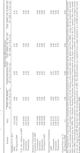
(9) List of Tables 1.1. Parameter values for the benchmark model and the model with frictions. 1.2. BUSINESS CYCLE STATISTICS- Perfect Risk Sharing model (benchmark. 51. model) and the Model with consumption habits, capital and labor adjustment costs 1.3. 52. BUSINESS CYCLE STATISTICS- Perfect Risk Sharing model (benchmark model) and the Model with consumption and leisure habits and capital adjustment costs. 1.4. 53. BUSINESS CYCLE STATISTICS- SENSITIVITY ANALYSIS- Economy with consumption habits, capital and labor adjustment costs. 1.5. 54. BUSINESS CYCLE STATISTICS- SENSITIVITY ANALYSIS- Economy with consumption and leisure habits and capital adjustment costs. 55. 2.1. Balance sheet of households if there is no sudden stop. 67. 2.2. Balance sheet of households if sudden stop occurs. 67. 2.3. Balance sheet of banking sector if there is no sudden stop. 69. 2.4. Balance sheet of banking sector if sudden stop occurs. 69. 2.5. Balance sheet of the government if there is no sudden stop. 71. 2.6. Balance sheet of the government if sudden stop occurs. 71. 2.7. Benchmark calibration. 80. 2.8. Benchmark calibration and intervals for the sensitivity analysis. 88. 2.9. Model variables and their data counterpart. 98. 3.1. Monetary and exchange rate regimes and in‡ation in CEECs vi. 106.

(10) 3.2. Consumer price index/Exchange rates correlations and coe¢ cients of variation. 107. 3.3. Null hypothesis: domestic block does not Granger-cause foreign block. 108. 3.4. Portmanteau test for autocorrelation (lag=12, no autocorrelation under the null hypothesis) and stability conditions. 109. 3.5. PPI’s variance decomposition. 110. 3.6. CPI’s variance decomposition. 111. 3.7. CPI’s response to one unit residual shock. 112. vii.

(11) List of Figures 1.1. Impulse response functions of home country variables implied by the model without any frictions. 1.2. 45. Impulse response functions of foreign country variables implied by the model without any frictions. 1.3. 46. Impulse response functions of home country variables implied by the model with capital adjustment costs, model with consumption habits and capital adjustment costs and model with consumption habits, capital and labor adjustment costs. 1.4. 47. Impulse response functions of foreign country variables implied by the model with capital adjustment costs, model with consumption habits and capital adjustment costs and model with consumption habits, capital and labor adjustment costs. 1.5. 48. Impulse response functions of home country variables implied by the model with capital adjustment costs, model with consumption habits and capital adjustment costs and model with consumption and leisure habits, capital adjustment costs. 1.6. 49. Impulse response functions of foreing country variables implied by the model with capital adjustment costs, model with consumption habits and capital adjustment costs and model with consumption and leisure habits, capital adjustment costs. 50. 2.1. Components of domestic absorption (standardized series).. 60. 2.2. Banking sector activity during the sudden stop with banking crisis (standardized series).. 61 viii.

(12) 2.3. Euro deposits withdrawal and foreign bu¤ers drop (mil. EUR) during the sudden stop with banking crisis.. 2.4. Short term foreign currency debt and euro deposits in % of foreign reserves in the period 1998-2008.. 2.5. 62. Reserves to short-term external debt ratio (%) and Reserves in months of imports.. 2.6. 62. 63. Benchmark calibration- Actual reserves, optimal reserves where parent banks act as the lenders of last resort (LOR), optimal reserves where parent banks participate in a crisis (mil. EUR).. 2.7. Decomposition of optimal reserves (mil. EUR) where parent banks act as the lenders of last resort.. 2.8. 82. 83. Decomposition of optimal reserves (mil. EUR) where parent banks participate in sudden stop.. 84. 2.9. Optimal reserves (mil. EUR) and kuna reserve requirenment relief (pp).. 85. 2.10. Actual and optimal reserves with Greenspan-Guidotti and 3-months-ofimports rules (mil. EUR).. 2.11. 86. Optimal reserves, Greenspan-Guidotti rule and 3-months-of-imports rule (mil. EUR) with di¤erent values of output loss (%).. 2.12. Optimal reserves, Greenspan-Guidotti rule and 3-months-of-imports rule (mil. EUR) with di¤erent values of fraction of deposit withdrawal (%).. 3.1. 86. 87. The EUR/USD exchange rate and the principal component of 9 CEEC (Romania and Slovenia not included) annual in‡ation rates. Both series are standardised.. 3.2. 100. Correlations beetwen CPI items (averaged across CEEC) and USD/EUR exchange rate.. 3.3. 113. Correlation between CPI in‡ation in Lithuania and the USD/EUR exchange rate.. 114. ix.

(13) Introduction This thesis consists of three self-contained essays. Although united under one title they di¤er in both the topics considered and approaches chosen. The …rst essay presents an international real business cycles model with real rigidities which today constitute a large part of closed-economy RBC theory in a complete markets setting. The second essay o¤ers a useful tool for central bankers in dollarized countries for analyzing foreign reserves adequacy. The third essay explores the impact of the USD/EUR exchange rate on in‡ation in the Central and East European countries (CEEC). In the lines which follow I give a brief overview of the three essays included into this thesis. Chapter 1, International business cycles with real rigidities in goods and factors markets, considers the importance of di¤erent types of rigidities, which today constitute a large part of closed-economy RBC theory, on international transmission of business cycles. In particular, I analyze the role of habits in consumption, capital adjustment costs and labor market frictions in form of habits in leisure or labor adjustment costs, in a standard international real business cycles (IRBC) model with complete markets. In this setting individuals have complete access to international risk-sharing (perfect risk sharing). The setup of my framework is similar to earlier two-country (two agents) IRBC models with complete markets in Backus, Kehoe and Kydland (1992) or Baxter and Crucini (1995)) except here a number of rigidities in goods and factors markets are incorporated. Because of complete markets setup the equilibrium allocation in this economy is computed as a solution to the social planner’s problem. The social planner’s problem was solved numerically using the parametrized expectations approach introduced by Marcet (1989). The main message of this paper is that the real rigidities that help explain many closedeconomy features resolve only the investment comovement puzzle. In particular, I …nd that capital adjustment costs together with consumption habits help to resolve the investment comovement puzzle by impairing capital ‡ows. Rigidities on the labor market do not help. 1.

(14) 2. explain factor comovements like the employment and investment puzzle. On the other hand, both labor adjustment costs and leisure habits increase the output correlation. However, only the e¤ects of the latter work towards resolution of the consumption cross-correlation puzzle (although not actually resolving it). This mainly comes as a result of leisure habits reducing consumption correlation through ampli…ed e¤ects on nonseparability between consumption and leisure. On the whole, real rigidities, either when resolving the investment puzzle or trying to resolve the consumption puzzle, accentuate problems in explaining other international comovements. Overall, Chapter 1 shows that real rigidities that help explain many closed-economy salient facts have less success in resolving international comovement puzzles. This conclusion supports the results of Kehoe and Perri (2002) or Yakhin (2007) that demonstrate the importance of …nancial and contractual frictions but also of some nominal frictions in explaining the international transmission of business cycles. In Chapter 2, Optimal Foreign Reserves: The Case of Croatia we analyze whether international reserves of the Croatian National bank (CNB) are su¢ cient to mitigate negative e¤ects of potential sudden stop of capital in‡ows and banking crisis. The need for reserves act as a protection against a sudden stop. This reserves requirement is even more pronounced in dollarized economies, like Croatian, where the central bank is exposed to a double drain risk (Obstfeld, Shambaugh and Taylor (2008)). This twofold risk exists given that …nancial account reversals (an external drain risk) may be accompanied by a loss of con…dence in the banking system that would result in a large withdrawal of foreign currency deposits (an internal drain risk). Therefore, in dollarized economy reserves are not only an insurance against negative e¤ects of a sudden stop but also a key tool for managing domestic …nancial instability. Our framework builds on analytical models trying to characterize and quantify the optimal level of reserves from a prudential perspective similar to those ones in Goncalves (2007) and Ranciere and Jeanne (2006). In our welfare-based model, precautionary motives for accumulating reserves pertain to the crisis management ability of the government to …nance underlying foreign payments imbalances in the event of a sudden stop and provide foreign exchange liquidity in the face of a bank run. At the same time the government is trying.

(15) 3. to maximize the welfare of the economy. In the model economy there are two main opposite forces driving optimal reserves accumulation. On one hand, reserves are expensive to hold. The cost of holding reserves might be interpreted as the opportunity cost that comes from substituting high yielding domestic assets for lower yielding foreign ones. On the other hand, reserves absorb ‡uctuations in external payment imbalances, ease the credit crunch and allow a country to smooth consumption in the event of a sudden stop with banking crisis. An analytical expression of optimal reserves is derived and calibrated for Croatia in order to evaluate whether the CNB holds more reserves than the model suggests are necessary. We …nd that for plausible values of the parameters the model accounts for the recent buildup of foreign reserves in Croatia. However, quantitative implications of the model imply that the accumulation of reserves was too strong. In other words, recent upsurge of reserves observed in Croatia over the past decade seems in excess of what would be implied by an insurance motive against sudden stop and banking crises. This result crucially depends on the assumed behavior of parent banks during a sudden stop. In working with data, we assume two possible reactions of parent banks during the crisis. parent banks might withdraw deposits and cut credit lines to banks in their ownership. On the other hand, they might act as a lender of last resort by prolonging short-term loans and providing extra liquidity. In the benchmark calibration we study optimal reserves in the economy that is hit by the sudden stop with banking crisis of the 1998/1999 crisis scale. We …nd that the CNB is holding enough reserves to mitigate negative e¤ects of a possible crisis similar to the one that took place during 1998/1999 only if parent banks assume the role of lenders of last resort. Finally, we compare our formula of optimal reserves with two standard indicators of "optimal" reserves for Croatian economy, namely Greenspan-Guidotti and 3-months-ofimports rules. We also show how using the two standard indicators of "optimal" reserves, the Greenspan-Guidotti and the 3-months-of-imports rules, might lead to an unrealistic assessment of the foreign reserves optimality in the case of Croatia. This result stems from the elements that determine optimal reserves and that Greenspan-Guidotti and 3-monthsof-imports rules do not take into account. In Chapter 3, The Impact of the USD/EUR Exchange Rate on In‡ation in CEE Countries we explore the impact of the USD/EUR exchange rate on in‡ation in the Central and.

(16) 4. East European countries (CEEC). The decision to analyze the USD/EUR exchange rate as a separate external factor is motivated by the monetary and exchange rate regimes in the CEEC. These countries are primarily concerned with ‡uctuations of their exchange rate against the euro: while all countries (will) have to participate in the ERM-II, some countries use the exchange rate against the euro (previously the Deutsche Mark) to reduce imported in‡ation and anchor in‡ation expectations. Since the USD/EUR exchange rate is determined on the global …nancial market, an individual country is unable to in‡uence it. Nor can it in‡uence world prices. Hence, it cannot simultaneously manage both its bilateral exchange rate against the euro and against the dollar. Therefore, for countries with heavily managed exchange rates to the euro, the USD/EUR exchange rate in fact represents an external shock. By focusing on the stability of their domestic currencies against the euro, the CEEC e¤ectively reduce the exchange rate pass-through of goods priced in euros to domestic in‡ation. However, since a number of commodities are priced in dollars, there is still a pass-through from the dollar, which is ampli…ed by the USD/EUR exchange rate ‡uctuations. We distinguish between the exchange rate of the domestic currency against the euro and the USD/EUR exchange rate and analyze which portion of the variation in in‡ation in the CEEC can be attributed to the USD/EUR exchange rate, as an external shock. In addition, we study to what extent USD/EUR exchange rate shocks in‡uence in‡ation. Finally, we attribute the di¤erent impact of the USD/EUR exchange rate on in‡ation among the CEEC to the di¤erent exchange rate regimes. To measure the impact of the USD/EUR exchange rate on domestic producers and consumer in‡ation across countries we employ the empirical model of pricing along a distribution chain, as in McCarthy (2008). The advantage of this model is that it has a Vector Autoregression (VAR) representation that allows us to trace the impact of exchange rate ‡uctuations on in‡ation at each stage along the distribution chain (importers, producers, consumers). While McCarthy (2008) studies a large open economy that can in‡uence external factors, we adopt a small country assumption where domestic variables cannot in‡uence external variables. In other words, we represent the model of pricing along the distribution chain in the CEEC with a VAR model with block exogeneity restrictions (for external variables) in the.

(17) 5. spirit of Cushman and Zha (1997). The imposition of block exogeneity seems a reasonable way to identify foreign shocks from the perspective of the small open economy. Our empirical exercise shows that the USD/EUR exchange rate accounts for the largest share of in‡ation volatility in the CEEC with stable exchange rates of the domestic currency against the euro. Furthermore, the extent of the USD/EUR exchange rate in‡uence on in‡ation in the CEEC is the largest in the economies with stable exchange rate regimes. This result might be important in the context of the price stability requirement of the Maastricht Criteria: in addition to the internal challenge of keeping low in‡ation and dealing with the di¢ culties of the price convergence process, the applicant countries could face problems beyond their in‡uence. Given that most of the CEEC peg their currencies to the euro, either because of the conditions of the Exchange Rate Mechanism II (ERM-II) or because of their domestic issues (eurozation in particular), and taking into account the high volatility of the USD/EUR exchange rate, our …ndings suggest that the CEEC under a …xed or heavily managed exchange rate might face substantial problems in achieving a high degree of price stability..

(18) References. Backus, D. K., P. J. Kehoe, and F. E. Kydland (1992): “International Real Business Cycles,”Journal of Political Economy, 100(4), 745–775. Baxter, M., and M. J. Crucini (1995): “Business Cycles and the Asset Structure of Foreign Trade,”International Economic Review, 36(4), 821–854. Cushman, D. O., and T. Zha (1997): “Identifying monetary policy in a small open economy under ‡exible exchange rates,”Journal of Monetary Economics, 39(3), 433–448. Goncalves, F. M. (2007): “The Optimal Level of Foreign Reserves in Financially Dollarized Economies: The Case of Uruguay,” IMF Working Papers 07/265, International Monetary Fund. Kehoe, P. J., and F. Perri (2002): “International Business Cycles with Endogenous Incomplete Markets,”Econometrica, 70(3), 907–928. Marcet, A. (1989): “Solving Stochastic Dynamic Models by Parameterizing Expectations,”Working paper, Carnegie Mellon University, Graduate School of Industrial Administration. McCarthy, J. (2008): “Pass-through of exchange rates and import prices to domestic in‡ation in some industrialized economies,”Eastern Economic Association, vol. 33(4), 511– 537 Obstfeld, M., J. C. Shambaugh, and A. M. Taylor (2008): “Financial Stability, the Trilemma, and International Reserves,”CEPR Discussion Papers 6693, C.E.P.R. Discussion Papers. Ranciere, R., and O. Jeanne (2006): “The Optimal Level of International Reserves for Emerging Market Countries: Formulas and Applications,” IMF Working Papers 06/229, International Monetary Fund. Yakhin, Y. (2007): “Staggered wages, …nancial frictions, and the international comovement problem,”Review of Economic Dynamics, 10, 148–171.. 6.

(19) CHAPTER 1. International business cycles with real rigidities in goods and factors markets 1.1. Introduction In a closed economy environment, real business cycle (RBC) theory has enjoyed a measure of success in accounting for many business cycle features. However, most of the poor matching performance of the standard RBC model came from the weakness of its internal propagation mechanism. During the past decade, several studies extended the standard RBC model to address this di¢ culty. The extensions were made via the introduction of di¤erent real rigidities in domestic markets for goods and factors of production. In particular, labor market rigidities such as labor adjustment costs (Cogley and Nason (1995), Janko (2008) and Chang, Doh and Schorfheide (2006)), habit preferences over leisure (Bouakez and Kano (2006), Wen (1998), Hotz, Kydland and Sedlacek (1988) and Eichenbaum, Hansen and Singleton (1988)) or the combination of habit preferences over consumption and capital adjustment costs (Boldrin, Christiano and Fisher (2001), Beaubrun-Diant and Tripier (2005) and Christiano, Eichenbaum and Evans (2005)) turned out to be important in magnifying the propagation of shocks in the economy. More recently Schmitt-Grohe and Uribe (2008) bring fresh news from the business cycles literature. By using the RBC model with real rigidities in terms of consumption habit preferences, leisure habit preferences together with capital adjustment costs they show importance of anticipated shocks as a source of economic ‡uctuations. Not only do all of these rigidities improve the matching performance of the standard RBC model, but they are now being used to understand a wide range of issues in asset pricing, growth, monetary and international economics1. 1 Several. papers are worth mentioning. Carroll, Overland and Weil (2000) suggest that consumption habits may be able to explain the relationship between savings and growth across the countries. Fuhrer (2000) argues that consumption habits can induce hump-shaped responses of consumption and in‡ation to monetary shocks. Mendoza (1991) …nds that introducing leisure habits in a small open-economy RBC model improves the …t of consumption and trade balance. Boldrin, Christiano and Fisher (2001) show that the combination. 7.

(20) 8. However, closed-economy models abstract from the fact that countries participate in international markets. In particular, they ignore that countries can have the opportunity to share country-speci…c risks with other countries through the exchange of goods and …nancial assets. An early open-economy version of the standard RBC model (international real business cycles models, henceforth IRBC models) that incorporated international linkages has been less successful than its closed-economy counterpart in replicating the basic characteristics of international comovements of output, consumption, investment and employment2. This model assumes the existence of complete markets that in turn implies perfect risk sharing among agents in the world economy. Perfect risk sharing has implications that are far away from the data. First, empirical cross-correlation of consumption is generally similar to cross-country correlation of output, whereas the standard IRBC model with complete markets produces consumption correlation that is much higher than that of output (consumption puzzle). And second, investment and employment tend to be positively correlated across the countries, whereas the model predicts a negative correlation (investment and employment puzzle). To reconcile data and theory models were developed in which risk-sharing is limited because of domestic or international …nancial frictions3. While much of the IRBC literature focuses on …nancial frictions for resolving international comovement puzzles, this paper explores the role of rigidities on markets for domestic goods and factors, which today present an important part of the closed-economy RBC model, on international comovements. In other words, I am asking the same question that Backus, Kehoe and Kydland (1992) put. of consumption habits, capital adjustment costs and labor adjustment costs helps to account for equity premium puzzle in the full-blown general equilibrium model. Janko (2008) …nds that labor adjustment costs are one of the factors that are crucial in explaining business cycle properties of real as well as nominal variables. 2 See, for example, Backus, Kehoe and Kydland (1992). 3 Baxter and Crucini (1995) and Kollmann (1996) investigated the quantitative impact of elimination of trade in state-contingent assets on the properties of international real business cycles. They found that the exogenous limit on the assets, that may be traded, was not severe enough in terms of risk sharing, investment ‡ows and working e¤ort to resolve correlation puzzles. Kehoe and Perri (2002) examined the model in which limited risk sharing arises endogenously from the limited ability to enforce international credit arrangements between the countries. They …nd that this contract enforcement friction goes a long way in reconciling the IRBC theory and data (although not all the way in terms of the consumption puzzle). Recently, Yakhin (2007) show that exogenous market incompleteness can also generate positive employment and investment cross-correlations once additional nominal rigidities are introduced (staggered wages and monopolistic behavior of households with respect to supply of labor)..

(21) 9. forward: what are the e¤ects of extending the standard RBC model to an open-economy environment. However, since from the time that the Backus, Kehoe and Kydland (1992) paper was published, much e¤ort has been devoted to extending the standard RBC model and trying to replicate salient features of the closed-economy business cycle. In order to explore the e¤ect of goods and factors market rigidities that represented those extensions on international comovements, I build a two-country IRBC model with habit formation preferences over consumption and adjustment costs on capital change in a complete markets environment. In this setting individuals have complete access to international risk-sharing (perfect risk sharing). In addition to consumption habits and capital adjustment costs, I analyze the impact of two labor market rigidities- demand-side rigidity in the form of habit formation preferences over leisure and supply-side rigidity in the form of labor adjustment costs. The main message of this paper is that the real rigidities that help explain many closedeconomy features resolve only the investment comovement puzzle. In particular, I …nd that capital adjustment costs together with consumption habits help to resolve the investment comovement puzzle by impairing capital ‡ows. Rigidities on the labor market do not help explain factor comovements like the employment and investment puzzle. On the other hand, both labor adjustment costs and leisure habits increase the output correlation. However, only the e¤ects of the latter work towards resolution of the consumption cross-correlation puzzle (although not actually resolving it). This mainly comes as a result of leisure habits reducing consumption correlation through ampli…ed e¤ects on nonseparability between consumption and leisure. On the whole, real rigidities, either when resolving the investment puzzle or trying to resolve the consumption puzzle, accentuate problems in explaining other international comovements. The rest of the paper is organized as follows. In section 1.2 I present a two-country IRBC model where habits and adjustment costs are incorporated in a complete markets environment. Simulation results together with interpretation of the results in terms of domestic and international (co)movements are presented in Section 1.3. Section 1.4 concludes..

(22) 10. 1.2. The model economy The model considered here follows closely the structure of earlier two-country IRBC models with complete markets (see, in particular, the models by Backus, Kehoe and Kydland (1992) or Baxter and Crucini (1995)) except here a number of rigidities in goods and factors markets are incorporated: habit formation preferences over consumption and leisure and adjustment costs on change of capital and on change of labor. In this section, I …rst describe the international environment of the model. Then I present a model as social planner’s problem. In the same subsection I provide and interpret the optimality conditions the solution of which the social planner has to satisfy and that I will use in order to simulate the same solution in the next section.. 1.2.1. The environment The world economy consists of two countries indexed by j = 1; 2; each populated with a continuum of identical households. Households in country j have preferences over consumption, cjt , past consumption incorporated in consumption habit stock, hcjt ,4 and labor, ljt , represented by the Von-Neumann Morgenstern expected utility function. Consumption habit stock evolves through standard law of motion characterized by a persistency parameter,. c. .. I also allow for two labor market rigidities and I analyze their impact separately demand-side rigidity in the form of leisure habits and supply-side rigidity in the form of labor adjustment costs. However, for the sake of compactness I will present the model as if both labor market rigidities are being analyzed at the same time. By shutting down the parameter characterizing each labor market rigidity, the model could be rewritten to incorporate each labor market rigidity separately. When I allow for demand-side rigidity in the labor market, households also have preferences over past labor incorporated in leisure habit stock, hljt . Leisure habit stock evolves through standard law of motion characterized by persistency parameters,. l. . In this case,. …rms decide on labor they want to hire, ljt , and investment, ijt . Firm’s capital accumulation technology is subject to capital adjustment costs governed by the function ( ). 4 The. particular speci…cation of preferences that I adopt links the household’s habits to its own past consumption ("internal habit"), rather than aggregate, economy-wide consumption ("external habit")..

(23) 11. On the other hand, when I introduce supply-side rigidity in the labor market, …rms decide on new hirings, mjt , in addition to the investment decision, which is subject to adjustment costs. Productive employment at time t + 1 is hired at time t. In deciding about new hirings, …rms take into account that on each occasion labor hours di¤er across periods they will face labor adjustment costs, governed by the function g( ). Furthermore, in each period exogenous destruction of hours worked occurs by the "quit" rate. 2 (0; 1). Hence,. changing employment within the …rm is costly, but it is costless to hire or replace the amount of employment that was exogenously wiped out. There is a single homogeneous good produced, consumed and used for investment by both countries. A country’s j output is produced using the technology that exhibits constant return to scale using capital, kjt and labor, ljt and is subject to country-speci…c labor augmenting total factor productivity shock, zjt . The countries are symmetric i.e. they share the same structure of economy in terms of preference, technology forms and parameters. Countries di¤er in two important aspects. In the …rst, labor input consists only of domestic labor (labor does not move across the borders). And in the second, production is subject to a country-speci…c (labor augmenting) technology shock. 1.2.2. The Social Planner problem I characterize the equilibrium in the world economy by exploiting the equivalence between competitive equilibrium and Pareto optimum with reference to the second welfare theorem5 (in Appendix 2 I show how to decentralize the social planner’s problem). Consequently, the equilibrium allocation in this economy can be computed as the solution to the social planner’s problem. The social planner chooses contingency plans for fcjt ; xjt ; ijt g1 t=0 in order to maximize the expected discounted sum of weighted utilities of the two countries j = f1; 2g. The control variable, xjt , denotes new hirings, mjt , in the case of analyzing supply-side labor market rigidity- labor adjustment costs, or just labor decision, ljt , in the case of examining demand-side labor market rigidity- leisure habits. The expectation is taken over the sequence of the shocks fzt g1 t=0 where zt = (z1t ; z2t ). 5 Note. that this is possible since, among other things, I am dealing with internal habits that, in comparison to external, do not exert any externality. For details see Alvarez-Cuadrado, Monteiro and Turnovsky (2004) or Alonso-Carrera, Caballe and Raurich (2004)..

(24) 12. I will present the model in "continuous" formulations in order to be consistent with the algorithm I use to solve the model- the algorithm utilizes a shock process that has continuous support. To do this, I …rst introduce some technicalities concerning the formal representation of uncertainty . Let (Z; Z) be a measurable space, where Z is a. algebra of the Borel subsets of Z.. Then the transition function can be de…ned as Q : Z. Z ! [0; 1] on (Z; Z) : It is assumed. that the transition function satis…es the Feller property. The sequence of the exogenous random vector fzt g is a Markov process generated by Q. Then, for a given point z 2 Z and a set A. Z, Q(z; A) can be interpreted as a probability that the next period’s shock lies in. A, given that the current shock is z: Next, I de…ne the spaces for the partial histories of shocks z t = (z1 ; z2 ; :::; zt ) ; for t = 1; 2; ::. Given a measurable space (Z; Z) a t fold product space (Z t ; Z t ) can be de…ned as Z t ; Z t = (Z. (1.1) where (Z :::. Z) denotes. :::. Z; (Z :::. Z)) ;. (t times). algebra generated by the product. algebras, for any …nite. t = 1; 2; ::: It follows that, for any given initial value of the shock z0 2 Z; and the transition function Q on (Z; Z), the probability measures spaces6. For any rectangle B = A1 (1.2). t. (z0 ; B) =. Z. A1. :::. Z. At. :::. 1. Z. t. (z0 ; ) : Z t ! [0; 1] can be de…ned on these. At 2 Z t ; let. Q(zt 1 ; dzt )Q(zt 2 ; dzt 1 ):::Q(z0 ; dz1 ):. At. In this economy, a consumption allocation, for both j = f1; 2g; is then de…ned as a. t t sequence of fcjt g1 t=0 ; where cjt : Z ! R+ is a Z - measurable function, for all t. In. a similar way, allocations of investment and labor supply, or new hirings are de…ned as 1 1 t t sequences of fijt g1 t=0 , fljt gt=0 or fmjt gt=0 respectively, where ijt : Z ! R+ , ljt : Z ! (0; 1). and mjt : Z t ! (0; 1) are Z t - measurable functions, for all t.. Then the objective of the planner is to solve the following problem:. 6 As. shown in Stokey, Lucas and Prescott (1989) (Section 7.5) it is su¢ cient to de…ne measurable rectangles in Z t :. t. (z0 ; ) over the.

(25) 13. max. fcjt ;xjt ;ijt g1 t=0. subject to: 2 X. (1.3). j=1. (1.4). 1 X. t. Zt. t=0. cjt +. Z. 2 X. ". ijt =. j=1. kjt+1 = (1. c l j u(cjt ; hjt ; ljt ; hjt ). j=1. 2 X. [f (kjt ; ljt ; zjt ). t. z0 ; dz t. g(mjt ; ljt )] ;. j=1. ijt kjt. )kjt + c. hcjt+1 = hcjt +. (1.5). #. 2 X. kjt ;. hcjt );. (cjt. 0. 1 c. 0. 1. in the case of labor adjustment cost: (1.6). ljt+1 = (1. )ljt + mjt ;. 0. 1. with kj0 ; hcj0 ; zj0 ; and lj0 given, for j = f1; 2g. or in the case of leisure habits:. hljt+1 = hljt +. (1.7). l. (1. ljt. hljt );. 0. l. 1. with kj0 ; hcj0 ; zj0 and hlj0 given, for j = f1; 2g Parameters. j. for j = f1; 2g represent the weights that the planner attaches to each. country. Furthermore, u( ) represents a utility function that is assumed to be bounded, continuos, strictly concave, strictly increasing and satis…es Inada conditions. f ( ) is a production function satisfying concavity and di¤erentiability properties. To …nd …rst order conditions corresponding to the planner’s problem, I rewrite the consumption habit stock as a function of all past consumptions: (1.8). hcjt+1 = hcjt +. c. (cjt. c. hcjt ) =. 1 X. (1. c i. ) cjt. i. i=0. and the leisure habit stock as a function of all past leisure hours: (1.9). hljt+1 = hljt +. l. (1. ljt. hljt ) =. l. 1 X i=0. (1. l i. ) (1. ljt i ).

(26) 14. Furthermore, I implicitly de…ne the investment function as (1.10). kjt+1. 1. I(kjt+1 ; kjt ) =. (1 kjt. i. )kjt. kjt. Then the optimality conditions that a solution of the planner’s problem has to satisfy are the following. The Euler equation for j = f1; 2g reads as: (1.11) (. u1 (cjt ; hcjt ; ljt ; hljt ). c. +. Z. Z. I1 (kjt+1 ; kjt ) =. Z. +. Z "X 1. c. 1 X. i. (1. c i. ). 2. i. c i. (1. ). #. u2 (cjt+i+1 ; hcjt+i+1 ; ljt+i+1 ; hljt+i+1 ). i=0. 4(f1 (kjt+1 ; ljt+1 ; zjt+1 ) + I2 (kjt+2 ; kjt+1 )) !#. u2 (cjt+i+2 ; hcjt+i+2 ; ljt+i+2 ; hljt+i+2 ). i=0. ). Q (zt ; dzt+1 ). 0. @u1 (cjt+1 ; hcjt+1 ; ljt+1 ; hljt+1 ). Q (zt ; dzt+1 ). The labor supply equation is given by: (1.12) gm (mjt ; ljt ) (. u1 (cjt ; hcjt ; ljt ; hljt ). (Z ". c. +. Z "X 1 Z. i. (1. ). #. u2 (cjt+i+1 ; hcjt+i+1 ; ljt+i+1 ; hljt+i+1 ). i=0. u3 (cjt+1 ; hjt+1 ; ljt+1 ) +. l. Z. ". c i. 1 X. i. Q (zt ; dzt+1 ). =. l i. ) u4 (cjt+i+2 ; hcjt+i+2 ; ljt+i+2 ; hljt+i+2 )+. (1. i=0. u1 (cjt+1 ; hcjt+1 ; ljt+1 ; hljt+1 ). +. 1 X. c. i. c i. (1. ). #. u2 (cjt+i+2 ; hcjt+i+2 ; ljt+i+2 ; hljt+i+2 ). i=0. 2. 4f2 (kjt+1 ; ljt+1 ; zjt+1 ). gl (mjt+1 ; ljt+1 ) + (1. 33. )gm (mjt+1 ; ljt+1 )55 Q (zt ; dzt+1 ). Finally, the risk sharing condition reads as: (1.13) u1 (c1t ; hc1t ; l1t ; hl1t ) + u1 (c2t ; h2t ; l2t ; hl2t ). ). +. c. R. R c. Z. Z. P1. i=0 P1 i=0. i i. (1. (1. 9 = ;. c i. ) u2 (c1t+i+1 ; hc1t+i+1 ; l1t+i+1 ; hl1t+i+1 ) Q (zt ; dzt+1 ). c i )u. c l 2 (c2t+i+1 ; h2t+i+1 ; l2t+i+1 ; ; h2t+i+1 ). Q (zt ; dzt+1 ). =. 2 1.

(27) 15. In those conditions ui (cjt ; hcjt ; ljt ; hljt ), fi (kjt ; ljt ; zjt ), Ii (kjt+1 ; kjt ); gi (mjt ; ljt ) denote the partial derivative of the function u( ), f ( ), I( ) and g( ) respectively, with the respect to the i th component variable. To sum up, in the optimum the world economy can be described by the following optimality conditions: Euler equations (1.11) and labor supply equations (1.12) for both countries j = f1; 2g and risk sharing condition (1.13) together with the budget constraint (1.3), laws of motion for capital, consumption habit stock, leisure habit stock (in case of examining demand-side rigidity in the labor market) or hours worked (in case of analyzing supply-side rigidity in the labor market) given in (1.4), (1.5), (1.6) and (1.7) respectively in each country. The optimality conditions that match up to the social planner’s problem help shed some light on the planner’s intratemporal and intertemporal allocation decisions. They demonstrate the dynamic characteristics of consumption, employment and capital in a framework with rigidities in labor, capital and goods market. In particular, for each country the Euler equation represents the planner’s intertemporal consumption trade-o¤: if the planner saves and invests one additional unit of the …nal good instead of consuming it today, she will consume more tomorrow as a result of higher capital stock to work with. But since the present utility of the planner is derived from past consumption also, which means that agents dislike variations in habit-adjusted consumption, rather than in consumption itself, reducing consumption today will come at the utility cost of u1 (cjt ; hcjt ; ljt ; hljt ), but also at the expected disR P1 i c i (1 ) u2 (cjt+i+1 ; hcjt+i+1 ; ljt+i+1 ; hljt+i+1 ) Q (zt ; dzt+1 ). counted utility bene…t of c Z i=0 Furthermore, one unit of …nal good saved today will not translate to a proportional increase of capital stock because capital is subject to capital adjustment costs (having a cost of I1 (kjt+1 ; kjt )) and to depreciation (represented by the cost of I2 (kjt+2 ; kjt+1 )). Each additional unit of production tomorrow, when used for consumption will yield utility bene…t coming from decreased consumption today but also utility loss because of habit forming preferences. The labor-supply equation shows planner’s intratemporal and intertemporal decisions on labor supply (leisure) and consumption in the general model with consumption and leisure habits and labor and capital adjustment costs. Since I am analyzing supplyside rigidity (leisure habits) and demand-side rigidity (labor adjustment costs) separately I will interpret the labor-supply equation by assuming that just one of the rigidity is present. Hence, if I allow only for labor adjustment costs (implying that utility is not derived from.

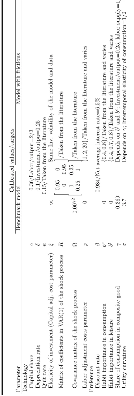
(28) 16. past leisure decisions), reducing new hirings today will come at the expense of labor adjustment costs, which will have both utility bene…t and utility cost. This opposite e¤ect on utility is the result of consumption habits, as in the Euler equation. Since labor hired today becomes productive only tomorrow, a fall in new hirings today will result in an expected discounted utility gain from increased leisure tomorrow. On the other hand, less hiring today will decrease productive labor stock tomorrow, part of which will be destroyed. A smaller labor stock tomorrow will produce less. This will again have a utility loss from present consumption and discounted expected utility bene…t from the future stream of consumption. If only leisure habits are present (and I neglect labor adjustment costs i.e. g(mjt ; ljt ) = 0) then labor employed today becomes productive immediately. Hence, reducing labor supply today will create a utility gain coming from increasing leisure activities today. On the other hand, this will come at the expected discounted utility loss coming from the future stream of leisure. Furthermore, a reduced labor force will produce fewer …nal goods which, when used for consumption, have again a utility loss from present consumption and a utility bene…t coming from the future stream of consumption. Finally, the risk-sharing equation requires that the ratio of marginal utilities of consumption in both countries has to be equal to the ratio of weights that the planner assigns to each country. 1.3. Quantitative model prediction To explore the quantitative impact of di¤erent rigidities for international comovements, the model has to be calibrated and functional forms have to be chosen. Before analyzing economies with rigidities, it is useful to review the mechanics of frictionless model (benchmark perfect risk sharing model) in order to understand the puzzles in the …rst place. I start by choosing the benchmark economy that is essentially a version of Backus, Kehoe and Kydland (1992), which has become the standard in the literature as a perfect risk-sharing case plagued with international comovement puzzles. I describe the calibration of the benchmark model in subsection 3.1. and that of the model with di¤erent rigidities in subsection 3.2. For the sake of comparability, when calibrating the model I build on the existing IRBC studies that take parameter values from growth observations or micro studies. If parameter value cannot be pinned down from the data, I choose its value such that the model’s second moment of some particular variable matches its empirical counterpart. If this is not possible,.

(29) 17. I adapt the parameter’s value from existing studies and then run the sensitivity analysis by varying the value of this particular parameter. The calibration procedure is summarized in Table 1.1. [insert Table 1.1 about here.] In this section I also brie‡y discuss the numerical algorithm that I construct for simulating the solution that satis…es the optimality conditions given in the previous section. In the end I provide the model’s …ndings and sensitivity analyses results from a simulation exercise.. 1.3.1. Functional forms and Calibration of the benchmark model As mentioned before, the world in my model is composed of two equally sized countries with identical preferences and technology and the same initial endowments so that the planner’s weights are the same,. 1. =. 2.. Following the previous IRBC literature I choose the functional. forms of preferences and technology (and the set of parameters values associated with these forms) to match the characteristics of the long-run behavior of aggregates observed in the U.S. data (for both j = f1; 2g). 1.3.1.1. Technology parameters. I use Cobb-Douglas production function (1.14). F (kjt ; ljt ; zjt ) = kjt (zjt ljt )1. which is consistent with the stability of labor share in output despite secular increases in the real wage. The parameter. represents the share of capital in output and zjt denotes. country-speci…c, labor augmenting total factor productivity (TFP) shock. The stochastic ‡uctuations of the TFP shocks of the two countries zt = (z1t ; z2t ) are assumed to follow a …rst order vector-autoregressive process, V AR(1); in logs. Letting Zt+1 = (log(z1t+1 ); log(z2t+1 ))0 the V AR(1) reads as:7 (1.15) 7 The. Zt+1 = RZt + "t+1 ;. transition function Q on (Z; Z) can be then de…ned implicitly by the assumption that the random shocks follow the stochastic di¤erence equation (1.15). See Theorem 8.9 in Stokey, Lucas and Prescott (1989) which insures that a …rst order stochastic di¤erence equation can be used to de…ne a transition function..

(30) 18. where f"t g1 t=0 is a sequence of bivariate normal random variables with zero mean and variance-covariance matrix. and where R is a autoregressive coe¢ cient matrix :. In general, TFP shocks can be related through the non-zero o¤-diagonal coe¢ cient of the matrix R and non-zero o¤-diagonal element of the covariance matrix. . In parametrizing. the coe¢ cient matrix R, I follow Baxter and Crucini (1995), Kollmann (1996) and Heathcote and Perri (2002) who found little evidence of spillovers between the United States and some European countries. Furthermore, as is common in the real business cycle literature I assume that each shock is highly auto-correlated. I summarize the parameters of the process given in (1.15) by: 2. R=4. (1.16). 0:95. 0. 0. 0:95. 3. 5;. 2. = 0:0072 4. 1. 0:25. 0:25. 1. 3 5. The later is consistent with the estimation results of TFP shock-processes for the United States and Europe8. The law of motion of the capital stock (1.4) in the steady state was used to calibrate the depreciation rate, , which depends on the investment/capital ratio that I restrict from observed data to take the value of 0:025 (as in Cooley (1995) I assume that the investment/output share in the US data is roughly 0:25, and that capital output ratio on a quarterly basis is around 10) (1.17). kss = iss. where subscript ss denotes the value of the corresponding variable in the steady state9. Hence. = 0:025:. The range of estimates for the capital share in the literature is compromise and set. 2 [0:25; 4]: I choose a. = 0:36 re‡ecting a long-run labor share in national income accounts. of 2=3.. 8 See. Backus, Kehoe and Kydland (1992), Baxter and Crucini (1995), Kollmann (1996) and Heathcote and Perri (2002). 9 Since I choose the same parametrization for both countries, they have the same deterministic steady state..

(31) 19. 1.3.1.2. Preference parameters. In the benchmark model economy, the preferences are of constant relative risk aversion form: (1.18) where. u(cjt ; ljt ) =. ljt )1 ] 1. [cjt (1. 1. 1. represents the curvature on utility, while denotes the share of consumption (relative. to leisure) in a composite consumer good. The discount rate, , was set so as to match the net average interest rate, (r. ) in the. US data of 6,5% (annual base). Using the Euler equation (1.11) in the deterministic steady state and shutting down all rigidities I have 1. (1.19) so that. 1 = 1 + ( kss 1 lss. ). 1 4. = [1 + (r. 1. )] 4. = 0:984:. The share of consumption good in the composite good, , was pinned down from the labor supply equation (1.12) in the deterministic steady state by shutting down all the rigidities and assuming that time devoted to market activities is equal to 1=3 and that the investment/output share is equal to 0:25. In the steady state the labor supply equation (1.12) reads as:. (1.20). css =. or by de…ning css = yss. lss )(1 (1. )kss lss ). iss and dividing by y I have. (1.21) from which I get. (1. 1. iss (1 lss )(1 = yss lss (1 ). ). = 0:369:. I calibrate the utility curvature parameter, , such that the intertemporal elasticity of consumption, IES(cjt ; cjt+1 ) in a deterministic model without any rigidities given as (1.22). IES(cjt ; cjt+1 ) =. 1. 1 (1. ).

(32) 20. is equal to 1=2. This value corresponds to the value of the curvature equal to 2, which is usually assumed in RBC and IRBC literature concerned with models without endogenous labor supply. Holding constant intertemporal elasticity of substitution and having calculated , I can pin down the curvature parameter,. = 3:7, corresponding to intertemporal elasticity. of substitution of consumption equal to 1=2.. 1.3.2. Calibration of the model with rigidities Once I have calibrated a benchmark model economy that does not include any rigidity, I present the calibration of a model with four di¤erent rigidities. Unfortunately, it was only possible to calibrate the capital adjustment costs parameter "properly" (such that the model’s investment volatility is equal to its empirical counterpart). In calibrating the parameters corresponding to other rigidities, I adapt their values from studies related to mine. In the sensitivity analysis I allow for these parameters to take di¤erent values in exploring how changes of these values a¤ect international comovements. 1.3.2.1. Capital adjustment costs. I use the speci…cation in Jermann (1998) to deal with adjustment costs to change of capital. Adjustment costs are governed by the function ijt kjt. where ( ) is a positive, convex function given by: ijt kjt. (1.23) Parameter. =. d1 1. 1. ijt kjt. 1. 1. + d2. represents the elasticity of investment with respect to Tobin’s q (ratio of the. price of a newly installed unit of capital to the price of investment good10). This parameter determines the magnitude of capital adjustment costs. Values for d1 and d2 are chosen so that the deterministic steady state is invariant to of Tobin’s q is equal to one. If. 11. ! 1 the capital accumulation formula reduces to the. 10 Note 11 The. i.e. so that the steady state value. that in the model without adjustment cost the Tobin’s q is equal to one. formulas are g1. =. g2. =. 1. 1 1. (1. ).

(33) 21. standard law of motion of capital without adjustment costs. I set the value for. so that the. investment volatility in the model is similar to that in the data. 1.3.2.2. Labor adjustment costs. In the case of analyzing supply-side rigidity on labor market , labor adjustment costs follow the standard quadratic speci…cation as suggested by Cogley and Nason (1995), Cooper, Haltiwanger and Willis (2003) and Shapiro (1986): (1.24) where '. g(ljt ; mjt ) =. ' ' 2 ljt+1 = (mjt 2ljt 2ljt. ljt )2. 0 denotes labor adjustment costs parameter. When ' > 0 …rms incur positive. labor adjustment costs in terms of loss of their production if aggregate hours worked di¤er across periods. There will be no labor adjustment costs if ' = 0 or if hours worked do not ‡uctuate across periods (for example, in the deterministic steady state).A functional form of labor adjustment costs is homogeneous of degree one. Hence, decision on hirings does not depend on the number of …rms, i.e. the assumption of a single representative …rm holds. Furthermore, the labor adjustment cost function is convex and symmetric. Convexity of the labor adjustment cost function has the same interpretation as convexity of capital adjustment cost function - changing labor stock rapidly is more costly than changing it slowly. Furthermore, symmetric property of labor adjustment costs could be interpreted as it is as easy to hire workers as it is to …re them12. The micro foundation of this kind of rigidity on the labor market stems from the fact that labor adjustment costs are just a particular case of a two sided search-and-matching process in the labor market. In particular, my model with convex labor adjustment cost, if put in a closed-economy environment, would be a particular case of the RBC model with two sided search and matching in Merz (1995) if the elasticity of job matches with respect to total search e¤ort were equal to zero, if a cost per unemployed worker is not incurred by varying search intensity and if posting a vacancy comes to an advertising cost that is governed by convex function13. As is usual in the RBC literature, my model yields employment volatility lower than in the data. Hence, no calibration of the labor adjustment costs parameter as in the case 12 I. also experimented with the natural assumption of being able to hire workers more easily than to …re them. Overall, the e¤ect of asymmetric labor adjustment costs were very small. Furthermore, notice that there is no actual …ring decision taking place. Employment is subject to continual exogenous depletion. 13 I am thankful for this comment to Thijs van Rens..

(34) 22. of the capital adjustment cost parameter,. was possible. I set the labor adjustment costs. parameter by referring to the labor adjustment costs literature. Cogley and Nason (1995) and Shapiro (1986) estimated a quadratic labor adjustment costs function similar to the one used here. Their …ndings correspond to the value of ' equal to 0:36. In a recent paper, Cooper, Haltiwanger and Willis (2003) estimated a similar quadratic labor adjustment costs function, obtaining a value of ' which is around 2. Given that the study of Cooper, Haltiwanger and Willis (2003) ) is more recent, I use this parameter value in simulating the model and in reporting my results. However, in order clearly to evaluate the impact of labor adjustment costs on international comovement, I conduct a sensitivity analysis with respect to ', and consider values of ' 2 f1; 20g as much smaller and much bigger value of labor adjustment cost parameter than the parameter value in the mail simulation exercise. The value of the quarterly exogenous quit rate is set to. = 0:15, based on micro evidence. reported in Andolfatto (1996). 1.3.2.3. Consumption and leisure habits. I assume simple time additive non-persistent habit-in-consumption speci…cation in the non-separable utility function14 (between consumption and leisure) proposed by Constantinides (1990). Then. c. = 1 in law of motion of. consumption habit stock(1.5). In this case, consumption habit stock at period t is simply represented by the level of consumption at period t. 1.. In dealing with leisure habits (bl 6= 0, see below) I assume the same habit-in-leisure speci…cation as for habit-in-consumption speci…cation. Then. l. = 1 in law of motion of leisure. habit stock(1.7). This non-persistent speci…cation of leisure habits found some support in empirical studies like Eichenbaum, Hansen and Singleton (1988), Yun (1996), Hotz, Kydland and Sedlacek (1988) and more recently in Schmitt-Grohe and Uribe (2008). Consequently, consumption and leisure habit stocks at period t are simply the levels of consumption and leisure at period t. 1. Then the utility function reads as:. (1.25) u(cjt ; hcjt ; ljt ; hljt ). 14 With. = u(cjt ; cjt 1 ; ljt ; ljt 1 ) =. (cjt. bc cjt 1 ) (1. ljt bl (1 1. ljt 1 ))1. 1. 1. additive habits the objective function of the planner preserves concavity property, whereas this might not be true in a model with multiplicative habits (see Alonso-Carrera, Caballe and Raurich (2005) for details)..

(35) 23. where bc and bl are consumption and leisure habit importance parameters. Now. denotes the. share of (habit adjusted) consumption (relative to (habit adjusted) leisure) in a composite consumer good. Again, the share of consumption good in a composite good, , was pinned down from the labor supply equation (1.12) by assuming that time devoted to market activities is equal to 1=3 and that investment/output share is equal to 0:25. But now in the deterministic steady state the labor supply equation (1.12) with additive non-persistent consumption and leisure habits reads as:. (1.26). 1. iss (1 lss bl (1 lss ))(1 ) = c l yss lss (1 )(1 b )(1 b). from which I get the value for. (1. bc ). depending on values for the habit importance parameters. bc and bl . Calibration of the habit model economy requires choosing a value for the habit importance parameter in consumption, bc , and, in the case of analyzing the rigidity on the demand-side of labor market , a value for the habit importance parameter in leisure, bl . There are several studies that try to estimate the parameter of consumption and leisure habits (see Diaz, Pijoan-Mas and Rios-Rull (2003) and Wen (1998) for an overview of the estimation of the consumption and leisure habit parameter, respectively). The conclusion of all these studies is that heterogeneity of data, techniques and goals in research rises to a very wide range of possible values for parameters bc and bl . Ideally, I would be looking for an estimator consistent with my model in functional forms and length of period, which does not exist. The range of estimated or calibrated values of bc and bl in the literature is very wide. Studies of asset pricing15, found that consumption habits characterized by values in the range of 0:69 to 0:9 can help to explain the equity premium puzzle. Since those models are close to mine, in reporting my results I use the a compromise between those values and set bc = 0:8. Finally, as far as leisure habits are concerned I follow empirical literature16 in parametrizing their importance parameter, bl = 0:7. In sensitivity analysis I report the results from simulation. 15 See 16 See. Boldrin, Christiano and Fisher (2001), Constantinides (1990) or Jermann (1998). Wen (1998), Hotz, Kydland and Sedlacek (1988) and Eichenbaum, Hansen and Singleton (1988)..

(36) 24. of the model with di¤erent combinations of two values of habit importance parameters (with the values that should correspond to low and high values of the parameter), bc = f0:4; 0:8g and bl 2 f0:4; 0:8g.. In the model with habits, again I calibrate the utility curvature parameter,. , such. that the intertemporal elasticity of consumption, IES(cjt ; cjt+1 )17 is equal to 1=2. In other words, I compare the benchmark economy and the economy with consumption and leisure habits but adjusted to have the same IES(cjt ; cjt+1 ). This is achieved by changing the curvature parameter, . Holding the intertemporal elasticity of substitution constant and having calculated. (depending on di¤erent values for bc and bl ) I can pin down the curvature. parameter, , which will now take di¤erent values for di¤erent values of bc and bl . Notice that in this way the steady state of the particular variable will be the same across di¤erent models and that simulated moments across di¤erent models will be comparable.. 1.3.3. Numerical solution of the model The social planner’s problem was solved numerically using the parametrized expectations approach (PEA henceforth) introduced by Marcet (1989). The idea of PEA is to replace the expectation functions in (1.11), (1.12) and (1.13) by smooth parametric approximation functions of the current state variables18 and a vector of parameters and then iterate on the values of parameters until rational expectation equilibrium is achieved. I choose PEA as a solution algorithm for two reasons. First, PEA circumvent the curse of dimensionality by avoiding the discretization of state space. And second, it has proven di¢ cult to compute a solution of models that incorporate additive consumption habits by value function iteration algorithm, for example. Diaz, Pijoan-Mas and Rios-Rull (2003) show that solving a simple growth model with exogenous incomplete markets and additive habits in consumption is not feasible. This is because the algorithm that relies on value function iteration cannot rule 17 Notice. that since I deal with additive consumption habits recalibration of the coe¢ cient of relative risk aversion in the model with habits is not needed since intertemporal elasticity of substitution of consumption in the model with habits is the same as in the setting without habits and it does not depend (in the deterministic steady state) on habit parameters bc and c . See Lemma 2 in Diaz, Pijoan-Mas and Rios-Rull (2003) that establishes this result in the environment without labor. It is straightforward to show that the same lemma applies to my model with endogenous labor supply decision and leisure habits. 18 In my model the vector of states is given by [k hc y z k hc y z ] where hc = c 1t 1t 1t 1t 2t 2t 2t 2t jt 1 for j = f1; 2g jt l and yjt = hjt = 1 ljt 1 in case of leisure habits or yjt = ljt in case of studying labor adjustment costs..

(37) 25. out ex ante the values of decision variables that the agent would try very hard to avoid (so that actually agents end up consuming negative habit adjusted consumption!). By the endogenous oversampling feature, PEA solves this problem. The endogenous oversampling feature implies that PEA only pays attention to those points that actually happen in the solution (for details see Marcet and Marshall (1994)) - only the economically relevant region of the state space is explored. For algorithm details see the Appendix. 1.3.4. Findings In this section I compare the quantitative properties of the theoretical world economy with those of the data. I start with a brief discussion of international comovement puzzles by comparing simulation results of a standard, complete markets IRBC model without any rigidity on goods or factors markets (the benchmark, perfect risk sharing model) with the moments calculated from the data (Table 1.2). Then, I explore the quantitative e¤ect of di¤erent rigidities on international comovements. In particular, I analyze the simulation results of two models: a model with consumption habits, capital adjustment costs and labor adjustment costs and a model that instead of labor adjustment costs incorporates a di¤erent type of labor market rigidity, namely leisure habits. First, I interpret the e¤ects of introducing capital adjustment costs and consumption habits both separately and jointly on international comovements in comparison to results of the benchmark model and data. Then, I investigate separate consequences on international correlations of introducing labor adjustment costs, on the one hand, and leisure habits on the other in the model with consumption habits and capital adjustment costs. Table 1.2 shows simulation results of the model that incorporates consumption habits (represented by parameter bc ), capital adjustment costs and labor adjustment costs (represented by parameter '). Table 1.3 shows the simulation results of the model that incorporates consumption habits (represented by parameter bc ), capital adjustment costs and leisure habits (represented by parameter bl ). By shutting down a particular parameter in two models, it is possible to explore separate e¤ects of a particular rigidity on international comovements. The statistics reported in all the tables in the …rst nine rows of the Data column are taken from Kehoe and Perri (2002) and pertain to the U.S. quarterly time series (logged and HP …ltered with smoothing parameter 1600). International correlations in those tables.

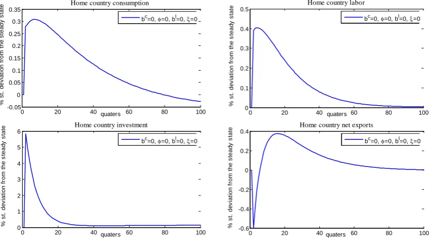
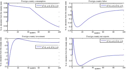
(38) 26. are also taken from the same source and refer to the correlations between U.S. aggregate variables and the same variables for the aggregate of 15 European countries. The capital ‡ow statistic was computed from the U.S. national accounts (NIPA) and pertains to the quarterly time series of net exports/GDP. To be consistent with the statistics computed from the data, the relevant model statistics are calculated from logged and HP …ltered data with smoothing parameter 1600. Instead of simulating each model many times to obtain many samples of arti…cially generated short time series and then calculating the average throughout the samples and its standard deviations, I simulated each model just once using however a long time series of each variable (10,000 periods)19. 1.3.4.1. The benchmark, perfect risk sharing model. In comparing the benchmark model and the data in the second and third column of Table 1.2, we can see three international comovement puzzles documented in the literature. In the model, consumption cross-country correlation is substantially higher than that of output (0.65 vs. -0.02), while in the data the opposite is true (0.32 vs. 0.51). And both investment and employment correlations are negative in the model (-0.78 and -0.37 respectively) whereas in the data they are positive (0.29 and 0.43 respectively). In addition, there is one major discrepancy in the domestic economy- both net exports and investments are much more volatile in the model than in the data (0.81 vs. 0.15 and 6.04 vs. 3.24 respectively). [insert Table 1.2 about here.] In order to get some intuition for the pattern of (co)movements of the model’s aggregates and the dynamics of the model. I study impulse responses of a world economy to a 1% increase in total factor productivity in the home country20 (pictured in Figure 1.1 and Figure 1.2). [insert Figure 1.1 and Figure 1.2 about here.] All the impulse responses of the aggregates are measured as percentage deviations from their steady state values. Figure 1.1 and Figure 1.2 illustrates what happens in the home and foreign country following a positive shock in the home country, which slowly dies out 19 The. two procedures should be equivalent assuming that number of simulations in the …rst and the sample size in the second procedure are large enough. 20 Notice that since there are no spillovers (a = 0) the productivity in the foreign country does not change. 2.

(39) 27. after the …rst period. Home investment and labor hours increase (resulting in an increase in domestic output) while foreign investment and employment fall (resulting in a fall in foreign output) - positive domestic productivity shock increases the productivity of capital and labor which results in a shift of resources to the home country. The capital stock in the home country increases both by domestic agents saving more and by more capital in‡ows from abroad taking advantage of higher return on capital in the home country. This will result in a negative cross-country correlation of investment. For our calibration of the model, investment rises much more than consumption and output together, leading to net exports de…cit and negative correlation of net-exports and GDP. With regard to employment, the temporarily high productivity of labor induces home country agents to supply more labor since the substitution e¤ect prevails over the wealth e¤ect, while in the foreign country the stronger wealth e¤ect of the shock generates a reduction in labor supply. This will result in a negative cross-country correlation of employment. Next, since country-speci…c risk is perfectly insured, agents in the home country agree to "share" some of the additional output generated by the increase in productivity in exchange for a similar deal when the other country receives a positive productivity shock. This will result in a positive cross-country correlation of consumption21 . Finally, large volatility of investment and net exports re‡ects the ability of agents in the model costlessly to shift investments across the countries (to a country which is more productive). 1.3.4.2. Adding capital adjustment costs. To account for variability of investment and net exports in the data I add capital adjustment costs into a benchmark model. Capital adjustment costs have been incorporated to slow the response of investment to a countryspeci…c shock. Without the capital adjustment costs, capital owners have a strong incentive to locate new investment in the more productive country making investment and then net exports excessively volatile. Here I compare the statistics of a benchmark model with those of the model where capital adjustment costs are incorporated. Table 1.3 presents simulation results of the model that 21. Note that consumption sharing between countries is not 1:1 because preferences are nonseparable in consumption and leisure making cross-country correlation of consumption smaller than 1. Actually, since consumption and labor are complements in utility function, consumption increases by more at home than abroad..