E
C
O
N
O
M
ÍA
SERIE DOCUMENTOS
B
BBOOORRRRRRAADADDOORORREESESS D
DDEEE I
IINNNVVVEEESSTSTTIIGIGGAAACCCIIIÓÓÓNNN
An approximation to the Standard of
Living Index: The Colombian Case.
Luis Fernando Gamboa Jorge Iván González Darwin Cortés
U
NIVE RSIDADDE L
R
OSARIOAn approximation to the Standard of Living Index: The Colombian Case
*Luis Fernando Gamboa♣
Darwin Cortés♣♣
Jorge Iván González♣♣♣.
Abstract.
This document seeks to show the main properties of a standard of living index using the theoretical approach of Amartya Sen. We establish the link among concepts such as: welfare, well-being, agency achievement and standard of living. Optimal scaling methodology was fundamental in order to test the properties on the Colombian case. These properties are Monotonicity, No independence of irrelevant alternatives, Concavity, Informativity and Substituibility.
Resumen.
El documento busca mostrar las principales propiedades de un indicador de estándar de vida dentro del enfoque teórico de Amartya Sen. Establecemos un puente entre conceptos tales como: bienestar económico, bienestar, logro de agencia y estándar de vida. La metodología del Optimal scaling fue usada para probar las propiedades de Monotonicidad, No independencia de alternativas irrelevantes, Concavidad, informatividad y sustituibilidad.
Keywords: Standard of Living, Optimal scaling, well-being, welfare, Prinqual
• This paper belongs to a large study of social policy financed by University of Rosario and FONADE. We want to thank Francisco Thoumi, Maria del Rosario Guerra, Monica Florez, Luis Eduardo Fajardo, Adriana Silva and Danielken Molina for their comments and help. However, all the mistakes are responsibility of the authors.
♣ Investigador Universidad del Rosario, Bogotá
Introduction.
The SISBEN is a social index created in 1993 and used by the Colombian government to select the beneficiaries of social programs, specifically in health. Its statistical methodology ranks households based on an index obtained from their life conditions (Castaño and Moreno, 1994). The Social Mission of The National Planning Department of Colombia (DNP) has developed, using the same methodology, a new and improved index named the Index of Living Conditions (ILC). ILC is the result of applying the Qualitative Principal Components (PRINQUAL) methodology to 9,121 households of the Quality of Life survey of 1997 (Encuesta de Calidad de Vida de 1997 (ECV-97)). ILC is an index composed of twelve qualitative variables organized in four factors which are related to some of the household’s living conditions.
In this index, the first factor gathers the characteristics related to public services that a given household has. In the second factor we can find the variables related to education. The third factor has demographic variables. And, a fourth factor is conformed by two variables that provide information about the materials used to build the house. Choice of variables depend on the objective pursued by researchers.
However, the efforts to conceptualize the I-SISBEN and the ILC started recently. The Papers that have worked on this subject can be classified by the theoretical basis used in two categories. On one hand, Velez, Castaño & Deutsch (1998) explained that these indexes show the level of utility reached by households. On the other hand, Sarmiento & Ramirez (1997), and Sarmiento & Gonzalez (1998) explained that these indexes show the household’ standard of living.
In this paper, we will explain the difficulties of the Utilitaristic Welfare approach and why the life level approach is more appropriate than the first one. Afterwards, we propose some properties that the standard of living indexes must fulfill and we will determine if the ICV index can accomplish them.
In order to talk about social policies, it is fundamental to have a theory that allows you to do interpersonal comparisons. The hypothesis is that any social political theory handles an implicit or explicit notion of distributive justice and it is only possible to talk about distributive justice when the theory allows you to do comparisons between individuals. Neoclassical normative economics do not allow these types of comparisons. In contrast, the conceptualizations done by A. Sen, enable these type of comparisons and they are appropriate for laying the theoretical foundations for social policies.
Agency, Well-being and Standard of Living1
As opposed to the neoclassic normative economy, Sen shows the necessity to do interpersonal comparisons. Public policy must enforce justice and cannot leave out interpersonal comparisons from the standard of living, welfare, or agency achievement.
1 We have differentiated the concepts: standard of living, welfare, well - being and Agency achievement. Other
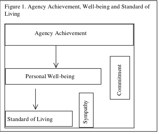
Figure 1 facilitates the comprehension of the meaning of standard of living and constitutes the difference proposed by Sen (1987 c, p 28). The most general concept is agency achievement (Sen 1985b). The freedom of being an agent is the biggest expression of liberty. The difference between personal well – being and agency achievement is commitment. The step between standard of living and well – being is determined by sympathy, or by antipathy. Sen proposes that the standard of living must be analyzed from the functioning and capabilities approach.
Well – being ideas cannot be separated from welfare ones. Both of them are inscribed in the welfaristic concept which centers its attention on welfare, in the sense that it supposes “the thesis that the only fundamental moral facts are facts about individual well-being (Sen 1985b, p.185). The welfaristic extreme approach reduces the welfare concept to its economic aspects. The only available information is utility. Sen’s main question is if utility is the only source of information for people’s welfare?
Sen (1987) says “It is useful to distinguish between two different critics that can be done of welfarism, in particular of taking utility to be the only source of value. First, it can be argued that utility is, at best, a reflection of a person’s well- being, but the person’s success cannot be judged exclusively in terms of his or her well-being.(…) Second, it can be disputed that personal well-being is best seen as utility rather than in some other terms”. Sen (1987, p.40). Sen develops his first critique in the distinction between the role of being agent and well – being. Commitment is the bridge between well – being and Agency achievement. The unique motivation for people is not to maximize their own well – being. The second critique brings into doubt the meaning of utility as the satisfaction of desire, happiness, or election. Sen’s concept of well – being is different from the utilitaristic tradition. The author shows that motivation’s heterogeneity, which conducts people’s lives, can’t be classified within welfare.
[image:4.612.72.334.173.395.2]Sen (1977, 1997) argues that commitment might answer to a scale of values very different from the scale that well – being uses. Up to the point that in many circumstances committed faithfulness causes indisposition. Sen shows a number of examples of disharmony between commitment and well – being. A swimmer who is seated in a small ship, decides to dive into the cold water in order to save a child that fell from a yacht. There’s no doubt that the rescuer’s fear and the cold water produce indisposition. But, once the child has returned to the yacht the swimmer feels satisfaction, the satisfaction of being a “free agent.” As in the swimmer’s example, Sen (1977) clarifies that commitment is not necessarily altruistic. A person can accept all the commitments that derive the agency freedom, because he aspires that in the future all the sacrifices experienced will result in a better individual well – being. There is no doubt the decision to study a career, or to study an art corresponds to agency freedom. But, the selfish
Figure 1. Agency Achievement, Well-being and Standard of Living
Agency Achievement
Personal Well-being
Standard of Living
Commitment
student might assimilate all the career displeasures because he is convinced that all is going to result in his personal well – being: he is going to be a famous, wealthy professional. In this case, commitment is related to individual well – being.
In graphic 1, it doesn’t matter if commitment answers to egoistic or altruist motivations. It is important to know that commitment makes the difference between personal well – being and Agency achievement. In the professional example, the concept of commitment has an intertemporal dimension that mixes present sacrifice with future well - being. Although the career choice is motivated by selfish principles, it expresses an agency success because the person accepts by his own will the privations that he ought to suffer while he converts into a famous and wealthy doctor.
Individuals are in continuous interaction, modifying preferences, and accomplishing moral and cultural responsibilities imposed by their beliefs. It is understandable that a person could have reasons to accomplish different objectives in his personal well – being. The well – being extension is founded in two criteria: The first one is the meaning that Sen attributes to the standard of living. It doesn’t depend on opulence, it depends on the functionings and the capabilities. Because of that, standard of living cannot be conceived from the utilitaristic perspective, which establishes a direct link between quantity of goods and utility level. The possession of goods is not translated into realizations or capabilities.
Sympathy is the second criteria required to proceed from welfare to “well being”. Welfare begins with the principle that individual welfare has nothing to do with another’s welfare. Meanwhile, “well – being” explicitly takes into account other people’s welfare. Sympathy is one of the ways that we can use to express the interdependence of well - being. Well – being of agent A is affected by agent’s B well – being. Although A has already reached a high standard of living in terms of functionings and capabilities, his well – being might decrease because B is suffering. To understand this difference, imagine a radical pacifist. Although he has a high standard of living, he seems very sad because he can’t rationalize why there are wars in different regions of the world. Well – being is also affected by antipathy. If A is a greedy person, he can’t enjoy his brand new car because his neighbor, mister B, just bought a better car. Sympathy or antipathy explains interpersonal comparisons. From another point of view, functionings that one person takes into account are what characterize this person’s life and well-being level.
Functioning is not only the act of owning goods, it introduces the idea of what people can do although they don’t accomplish them with the goods they own. “the central feature of well being is the ability to achieve valuable functionings” (Sen 1985, p.200). It’s important to mention that functionings can be influenced by society.
In brief, the non-utilitaristic well-being appreciation, does not conceive standard of living as a utilitaristic view. From Sen’s perspective, the standard of living refers to the valuation of one person’s capabilities and functionings, without taking into account other’s sympathies or antipathies that affect well – being.
SOME STANDARD OF LIVING INDEX PROPERTIES
We are going to explain some of the properties that, in our opinion, standard of living level indexes must have.
One person’s standard of living is related to the realization vectors that he might choose. The vector valuation is done by taking into account the type of life that a person has. But, identifying what a person can do is impossible. It is necessary to choose an object value that can be used to evaluate standard of living. The selection of the value objects is a valorative exercise of the standard of living.
The value objects involved in the ILC index refer to the household’s living conditions. These characteristics limit the index. It doesn’t capture the inequalities among households (gender discrimination, child abuse, etc.).
ILC obtains information from value objects (capabilities and functionings) through different variables that measure the level of people’s lives. The components of the index are very important because they inform what people have. ILC includes information about people’s belongings (house construction materials, education, etc.). ILC provides information about what people can or could do. We ought to find a function that can provide a common pattern to value the standard of living of different people.
ILC has a cardinal metric that enables us to order households in a standard of living level function. It is not a well-being index because it doesn’t capture in a direct way sympathies or antipathies. It does not capture the impact of agent B’s well – being over that of agent A.
As we say above2, ILC is composed by qualitative variables and the ILC of each household is expressed by:
(1)
∑∑
= =
=
Ff C j
i fj fj f i
f
v
w
W
ILC
1 1
2 Castaño and Moreno (1994) explained the statistical methodology to obtain ILC. Included variables are
RECOBA = Disposal of Garbage EXCRET = Type of toilet
CONQCOCI = Fuel most often used for cooking ABAGUA = Main source of water
ESP12YMA = Average schooling of household members 12 years and older. ESMXJEFE = Schooling of head of household
PROSEC = School Attendance of 12 – 18 years old individuals YPERCAP = Per capita income
PROP6 = Proportion of children 6 years or younger HACICUAR = Overcrowding
where wf is the weight associated to factor3 F, W0 is the weight of variable j that belongs to
factor F, vifj is the valuation that receives household i in the category of the answer4 that belongs
to the j variable of Factor f. F is the factor number, and Ct is the number of variables in each
factor.
Property 1: Independence of irrelevant alternatives
The Arrow (1951) social welfare functions (SWF) ought to fulfill the independence of irrelevant alternatives property. The welfare social function corresponds to well – being because its arguments are the status of the world. Property 1 is defined in a different space from life condition. The exercise of obtaining a function that provides a common pattern to measure people’s standard of living is different from the exercise of judging between the social status from individual preferences. The common standard of living measure doesn’t resolve the interpersonal conflict when you are trying to measure social status. The fact that two different agents have the same function valuing the standard of living, doesn’t mean that they order their social status in the same way. Ordering of social status is influenced by the agent’s equity criteria, and the place where each social status happened. These individual aspects might be different among two agents that have the same standard of living function.
The Arrow (1951) condition of independence of irrelevant alternatives does not have a meaning when you are trying to build a function that assigns values to the individual life standard.
Independence of irrelevant alternatives can be written as: R and R’ are social binary relations defined by a rule of collective selection f, which corresponds one to another through a different individual preference, (R1, …Rn) and (R’1, …R’n). If for all pairs of alternatives x, and in a
sub-conjunct S that belongs to X, where xRiy xR’ i y, for every i, so all the status of the world
which are as good as all the other world status of conjunct S, they are the same for both orderings R and R’.
In property 1, we distinguished the aspects related with the ordering of irrelevance. The ordering means that in the social choice between social states x and y, the only relevant information is the one that comes from individual orderings. The irrelevance is used to explain that social selection between x and y is not influenced by individual orderings of another variable z respect to x, y or other variable.
In our case, we are not interested in selecting between social states x and y. We are interested in making a function that values the agent’s life conditions. We can ask if a version of property 1 defined in a proper way is plausible or not. In this version, the ordering might be associated to an informational restraint. This restraint implies that agents might order the realization vectors,
3 The factors are sets of variables introduced in the index. The variables that belong to a Factor are correlated
among them, but they are little correlated with variables from other Factors.
4 Each variable has different categories. For example, the variable Type of toilet has four categories: No toilet,
and their value might come from this ordering. The irrelevance explains the reason why the realization vector x is independent from the other vectors.
When we talk about ordering it is necessary to know that the informative well - being basis and the people’s standard of living are plural. There is another type of information that comes from the ordering which is relevant to assign the values to functionings. For example, freedom associated with certain kind of realization vectors affects the value that the vector receives. Freedom extent is associated with the extent of the functioning vector set and the way in which these vectors are valued. Amplifying the relevant information set to establish the judgments over well – being influence the possibility to order the functioning vector. We could only make judgments over the standard of living with respect to a subset of realizations, but we will not know which one has the higher valuation.
When we refer to the irrelevance of property 1 we have to recall that an individual’s well – being depends on the success and the freedom of well-being. The realization vector and the set of functionings are very important. It is not the same to choose not to eat because of religious beliefs than to choose not to eat because you don’t have the money.
Capabilities and functionings are very important for the people’s standard level and they play a different role. “A functioning is an achievement, whereas a capability is the ability to achieve” (Sen 1987c, p 36). Functionings are more related to the living conditions, and the capabilities of freedom are more related to the real opportunities that an agent has. This doesn’t mean that capabilities have nothing to do with standard of living level. The valuation of the lifestyle of an agent is influenced by the different types of lives that he can conceive. In the same way, people’s realizations depend upon the decisions they make. Functionings influence capabilities (freedom as people’s real opportunities). There is a bi-directional relation between functionings and capabilities that needs to develop as a way of evaluating the standard life level introducing considerations about freedom.
Because of that, the condition of independence of irrelevant alternatives doesn’t have a plausible interpretation that can lead to build a standard level function. All the alternatives are relevant because they affect people’s freedom and realizations.
Property 2: Informativity
This property is deeply related to two questions. Which is the relevant information set used to construct judgments of life standard level? And What information does the ILC index provide?
It is important to recognize if the index of standard of living captures the effects of social policy over the standard of living level and if so, it is important to see how it does this. One of the biggest difficulties of other social indexes such as the poverty line is that the effects of social policy are not captured or the effects are captured in the wrong way. In the short run social policy might affect standard of living level without affecting a household’s incomes (for example, investing in education). It is desirable that improvements and impairments of the agents living conditions affect the index in the desired way.
Property 3: Concavity
Standard of living level must be concave with respect to its arguments. Concavity means that the improvements of life conditions increase the ICV index more in households with minor living conditions level.
It is possible to analyze this property under two ways, the theoretical and the empirical way. The theoretical analysis is done through the characteristics of the mathematical function. The empirical analysis is done using the household’s index results.
As we can see in expression (1), ILC is a linear combination of the variables vifj. Therefore, the
function is concave and weakly convex. Unfortunately, the values of the variables vfj depend
upon the household’s category in such variables. As an example, the variable water supply receives different values if water is supplied from a river, or if the water is supplied through the aqueduct. This is the reason why we can assume that variables are a function of the categories that conform5 the variable.
(2)
( )
fj k fj fj
fj c v v v c
v : → , =
where ckfj is the category k of variable j of factor f.
Substituting expression (2) in expression (1) we get:
(3)
∑∑
( )
= = = F
f C
j
k i fj fj f i
f
fj
c v w W ILC
1 1
Now we will analyze if ILC is concave with respect to the categories of the ck variables. In this
case, Wf and wfj are positive numbers, so it is only necessarily to show that each of the vifj(ckfj)
functions are concave. If they are concave ILC will be concave too.
Concavity requires that the individual categories contain continuity between each other. During the education years this continuity is organized: from 3rd grade it goes to 4th, from 4th grade it
5The categories of each variable are established with the criteria of differentiating the population by their standard of
goes to 5th, and so on. But there are other qualitative variables like the water supply, that don’t show a scale of continuous categories. The presence of discrete intervals, makes the function of the ILC non-continuous with respect to the variables categories, so the function in not concave6. The empirical analysis is going to be done by municipal averages, therefore we avoid the continuity problem.
Property 4: Substitution
Standards of living among agents are not all the same. The possibility that people have to accede to distinct goods is different. Although people can have the same capabilities, they don’t translate into the same functionings. The living conditions that individual households have are not equal. When there are different endowments, different capabilities, and different interaction systems among people, it is quite probable that there are different living conditions. The heterogeneity of aspirations and possibilities influences people’s abilities and functionings in different ways. Therefore, it could happen that for one well – being example, you could find various conditions and different standard life levels. When you work variables such as income into the line of poverty index there is no certitude that people expend their income in what they ought to spend it (for example, in the satisfaction of basic needs). The ideal standard of living is not the same for everybody. Functionings change, even though the capabilities and the goods vector are still the same.
The substitution property is very important, because the ILC is a compound index that involves different living conditions. It allows in some instances that different agents can be more effective in certain situations than in others.
Property 5: Monotonicity
A standard of living index must be monotone. This property establishes a relationship between the values assigned to the variables introduced in the analysis, and the household’s standard level. This property can be expressed in such a way that it involves comparisons between households (or municipalities).
Formally,
j i j
i j
i j i m j
i vf vf vf vf vf ILC ILC vf vf
f v
v f v v
v v v v
v
→ >
→ > ≠
∧ ℜ ∈
∀ , + , ( ) for
i
,
j
households (ormunicipalities) e
i
≠
j
where; household i has a higher standard of living level than the standard’s of household j. If and only if, household i has at least one characteristic that is valued higher (the others receive the same valuation) than in household j.
Assuming these parameters, the index is going to accomplish this characteristic. But this characteristic can be reached in other cases. In general, the index accomplishes this
characteristic whether the order of the variables are the same as the order given by valuations. The index is a sum of the valuations of the variables, so if all the agent’s valuations except one are equal to another’s agent valuation, the best index is the one where the different valuation is higher. This is a clear advantage of the index due to the way in which it is calculated.
Monotonicity may be expressed with respect to changes in the household’s standard of living level.
i i i
i i
i i i m i
i vf vf vf vf vf ILC ILC vf vf
f
v , ' ' , ' ( ' ) '
v f v v
v v v v
v
→ >
→ >
≠ ∧ ℜ ∈
∀ +
for living conditions vfvy vfv' of household (or municipality) i.
Where, household i has a higher standard of living level in state x than in state y. Household i has at least one characteristic (other characteristics have the same valuation) that is valued higher in state x than in the other state. Given the parameters, monotonicity is guaranteed by the way in which the index is constructed. But if valuations change, monotonicity might not be able to accomplish this. The weight of the variables is the unit of measure of the index. When the weights change, the metric (the final valuation of the variables) changes, too. So, it is more difficult to do dynamic comparisons with this index. If we want to make it possible to do intertemporal comparisons, it is necessary to keep the unit of measure constant.
Statistical Exercises
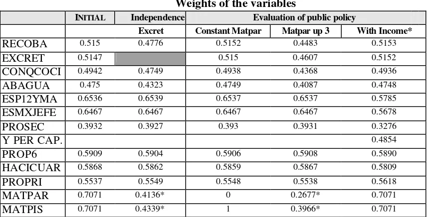
As we show above, ILC is the result of the optimal scaling methodology that determine different weights for the variables included. And as long as we keep improving within the categories, the final valuation is better. This means that the ILC score increases with the standard of living level without being normative, because we didn’t define a – priori ideal conditions. This characteristic is the main difference between ILC and other compound indexes, like the NBI that has the same weight for each variable. In the first column of table number 1 we can see the weights of each variable that was studied.
Another characteristic is that ILC is robust for the size of the studied population and with the information that was taken into account in the exercise. To prove it, we did two types of exercises. Some of them excluded households, while others excluded variables. When we repeat the estimate with fewer households or with fewer variables, the robustness and the reliability of the test was confirmed. The variables not excluded maintain the structure of the index. The reduction of households used in the estimate began to affect the index when it reached more than 50% of excluded households.
Table No. 1 Weights of the variables
INITIAL Independence Evaluation of public policy
Excret Constant Matpar Matpar up 3 With Income*
RECOBA 0.515 0.4776 0.5152 0.4483 0.5153
EXCRET 0.5147 0.515 0.4607 0.5152
CONQCOCI 0.4942 0.4749 0.4938 0.4368 0.4936
ABAGUA 0.475 0.4323 0.4749 0.4087 0.4748
ESP12YMA 0.6536 0.6539 0.6537 0.6537 0.5785
ESMXJEFE 0.6467 0.6467 0.6467 0.6467 0.5678
PROSEC 0.3932 0.3927 0.393 0.3931 0.3276
Y PER CAP. 0.4854
PROP6 0.5909 0.5904 0.5906 0.5908 0.5890
HACICUAR 0.5868 0.5862 0.5859 0.5867 0.5809
PROPRI 0.5537 0.5549 0.5548 0.5538 0.5618
MATPAR 0.7071 0.4136* 0 0.2677* 0.7071
MATPIS 0.7071 0.4339* 1 0.3966* 0.7071
Source: ECV-97. Estimated by the authors . *Goes to Factor 1.
To prove the first two properties, we evaluated the effects of some changes made to the weights of variables and the factors. We also tested the contribution of each variable and factor to ILC. In table 1, we summarize some of the results obtained to test the independence of irrelevant alternatives and the ILC informativity.
We evaluated the independence of irrelevant alternatives by using an exercise that measures the impact on ILC if one of its variables is eliminated. If we exclude one variable, it is necessary to re-estimate the weights of factors, and the rest of the variables used. We did twelve (12) sets of weights. Each weight was estimated leaving out a different variable.
In the first column of the next table we compare the results with the initial weights. We only show the case where variable EXCRET was eliminated. We observe changes in the weight and in the number of factors7. The importance of the order of the Factors was affected too (if you organize the factor from highest to smallest). This result suggests that the present variables of ILC are relevant and their absence affects the relative weight of the variables not excluded.
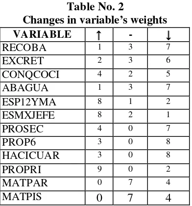
The weights changed in almost all the cases, which can be understood as a variation of the orderings. When a variable of a given factor was excluded, the other factor variables were responsible for explaining the total variance of the factor. When a factor had only two variables and we took one out, the variable left in the model assumes the value of one (1). In three cases, the variables from the fourth factor became part of the first factor. That’s why you can’t find the weight of the fourth factor in the table.
Table No. 2
Changes in variable’s weights
VARIABLE ↑↑ - ↓↓
RECOBA 1 3 7
EXCRET 2 3 6
CONQCOCI 4 2 5
ABAGUA 1 3 7
ESP12YMA 8 1 2
ESMXJEFE 8 2 1
PROSEC 4 0 7
PROP6 3 0 8
HACICUAR 3 0 8
PROPRI 9 0 2
MATPAR 0 7 4
MATPIS 0 7 4
Source: ECV-97. Estimated by the authors.
Table number two (2) summarizes the changes in the variables weighs. Informativity was tested by three exercises that were similar. But, they help to evaluate the effects of different levels of intensity of public policies. The first exercise assumed a successful program was carried out by the government in an specific area, where all the families were even. The second exercise judged the effect of a program implemented only in the lowest households. Finally, we evaluated the impact of including the income in ILC. This exercise is the same as comparing the ICV with the I-Sisben. The weights calculated for variables and factors are in columns 3.4 and 5 of table 1.
We assume that a public policy must improve the living conditions in at least one of the categories. We simulated the impact of a program that improves the materials used to construct the walls of all the houses. This is the same as considering the ICV in another time state.
As we can see in the column named “Matpar constant” of table 1, the weight of this variable changed from 0.7071 up to zero (0). The weight of the floor material that belongs to the same factor increases up to one, because from now on it is going to be responsible for explaining the total variance associated to this factor. Although the others weights changed, the variation is so insignificant that it doesn’t modify its order8.
From this exercise we obtain two conclusions. The index captures the equality between households prior to applying a variable, reducing its weight. This reduction will happen again if households are adjusted to the worst level or if a natural disaster occurred.
The second exercise suppressed at least one of the lower categories of any variable. We assumed in this exercise that public programs have a lower impact than the last one. The answer category set of the variable is reduced. When two categories were leveled, the last two disappeared. So
8 We did the same exercise with an alphabetization policy that leveled the house heads education level and the
the households were re-located in the following two categories. The exercise was done for MATPAR, ESMXJEFE and ESP12YMA, but we only showed the results of the first case.
In the fourth column of table number one (1), we can find the final weights of the factors and the variables. There are two effects that we have to take into account. When the program improves three levels in MATPAR, the fourth factor disappears. The variables that measure the floor of the house, and the house walls are now part of factor one (1). The factors kept the initial ordering. As such, this type of public policy is captured by the index through the changes in the index structure (there are changes in the weights and the components of the Factors)
The third exercise introduced income. The inclusion of income is the principal difference between I-Sisben and ILC indexes. The first one incorporates income, and the second one doesn’t. Income was introduced as a categorical variable, conforming intervals.9 Income is a part of the second factor, where we can find the variables that are related to education. The second factor gains relative importance in two points, which are lost by the first and the fourth factors. None of the factors suffered an important loss (gain) in its weigh (Wf). The change is
small if we take into account the importance attributed to income in other social indexes, like the poverty line index or the Gini Coefficient, or the HDI. See graphic 2.
From these results, we can say that it appears income is not an important variable in the ILC index. We consider it relevant to compare the results obtained by the ILC index at the beginning with the results obtained when income was introduced. To do this, we run a model of the form:
ILCi =(ILC,E)
Where:
ILCi: Is the score reached by households when income is introduced.
ILCj: Is the score reached by households without taking into account the per capita income.
E : is the residual
The results of the regressions show that there is a high correlation between the ILCi, and the
ILCj. This shows that there isn’t an important change in ICV when the income is introduced.
The ILCj index is significative , and the high r2 guarantees the existence of correlation between
the two models.
DIAGRAM 1
ILC With and without income.
0 10 20 30 40
0 20 40 60 80 100
ILC
% of the people
ILC (without income) ILC (with Income)
Source: ECV-97
ILCi = -0.585332 + 0.975055 ILCj
(0.07500617) (0.00099)
F : 951793.64 R-square 0.9906
Source: ECV-97. Estimated by the authors.
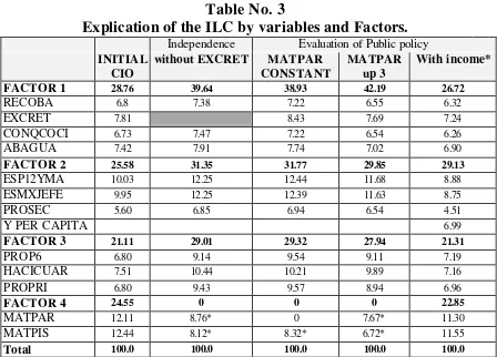
When we change from the I-Sisben index to the ILC index, two problems are solved. The first one is related to the complexity of the notion of income. The second one is that income can be deducted from other variables associated with the households living conditions. It is convenient to analyze how the explicative structure of the index changes, understanding it, as the contribution of each Factor and each variable to ILC.
Analyzing the independence property, the modifications suffered by the weighs of variables (wfj)
Table No. 3
Explication of the ILC by variables and Factors.
Independence Evaluation of Public policy
INITIAL CIO
without EXCRET MATPAR
CONSTANT
MATPAR up 3
With income*
FACTOR 1 28.76 39.64 38.93 42.19 26.72
RECOBA 6.8 7.38 7.22 6.55 6.32
EXCRET 7.81 8.43 7.69 7.24
CONQCOCI 6.73 7.47 7.22 6.54 6.26
ABAGUA 7.42 7.91 7.74 7.02 6.90
FACTOR 2 25.58 31.35 31.77 29.85 29.13
ESP12YMA 10.03 12.25 12.44 11.68 8.88
ESMXJEFE 9.95 12.25 12.39 11.63 8.75
PROSEC 5.60 6.85 6.94 6.54 4.51
Y PER CAPITA 6.99
FACTOR 3 21.11 29.01 29.32 27.94 21.31
PROP6 6.80 9.14 9.54 9.11 7.19
HACICUAR 7.51 10.44 10.21 9.89 7.16
PROPRI 6.80 9.43 9.57 8.94 6.96
FACTOR 4 24.55 0 0 0 22.85
MATPAR 12.11 8.76* 0 7.67* 11.30
MATPIS 12.44 8.12* 8.32* 6.72* 11.55
Total 100.0 100.0 100.0 100.0 100.0
Source: ECV-97. Estimated by the authors . *Goes to Factor 1.
In the third table, we can observe how the first Factor reaches the higher explicative levels, while the last Factor has the lowest ones. When we worked with the informativity property, the initial political variable is MATPAR, and it makes MATPIS form part of Factor 1, gaining up to 50% of the ICV. The increase in the other factors is lower, and they conserve the same order of importance in it’s application.
The variables of Factor four have lower weighs than the initial ones. So, the contribution of each variable in the ILCV decreased.
To prove the concavity of the index, we must remember that every concave function is quasi-concave, but not every quasi-concave function is concave . The model used a Trans-logarithmic function, which has the advantage of not supposing an a-priori concavity of the function, like the Cobb – Douglas function does. We began our analysis attempting to discover if the function was quasi-concave or quasi-convex in Factors and in variables. Because the index gathers the variables in four factors, the first regression took the form of:
∑∑
∑
= = =
+ +
+
= 4
1 4
1 4
1
ln ln ln
ln
f j
j f fj f
f
f F b F F
a A
Where F is the Factor and e is the residual.
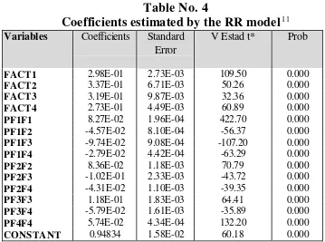
Estimating by Least Squares, the residuals had a high Kurtosis, so it is possible to believe that they follow a double exponential distribution. Because of that, we used a robust regression with the criteria of Least Absolute error. The adjustment of the model was excellent, the R2 (estimated and observed) was equal to 1.000, and the FACTf estimated coefficients are congruent with the index structure (they are positive and significant) (See table 4).
Using the FACTf coefficients we applied the determinant criteria to accept or refuse the quasi-concavity hypothesis of the function. Evaluating the principals, we saw that they were negative (near zero), so we can’t affirm that the ILC is quasi-concave in Factors, so the index is not concave in the Factors. Using the same methodology as before, we proceed to verify that ILC was concave in variables, but with the difference that now we have more variables incorporated. We used 12 variables in the model, so the regression had the following form:
∑∑
∑
= = =
+ +
+
= 12
1 12
1 12
1
ln ln ln
ln
i j
j i ij i
i
i V b V V
a A
ILC ε
Where ILC is the Living Conditions Index for the municipalities, and V is the municipality mean for the correspondent variable.
The model adjustment is still excellent, R2 is equal to 1.000 (observed and estimated), and the coefficients estimated are all significant. With these results we constructed a Hessian matrix of the variables10, and again, there is no quasi-concavity in variables, so the function is not concave in variables.
The question we ought to answer is what did we use to produce a function that is not concave? First of all, we used the ILC’s municipality mean, which fails to incorporate the idea of marginal gains that a household could have, as a result of an improvement in its standard of living level caused by the positive changes in the household conditions. Second, it is not always true that differences between the final valuations diminished as living conditions are improved.
Finally, to prove substitutability, we assume that all the households with the same score in ILC, do not have the same living conditions. If there is substitutability, two or more households with similar life levels could have alternative life conditions. This is a very important aspect because it reaffirms the normative ILC characteristic. Households choose goods that will give them alternate life conditions, so it replaces one with another. For example, you can compensate a bad quality wall material with a higher level of education, but it is necessary to take into account that capabilities and surroundings among households are very different. Fulfilling substitutability, we can avoid homogenizing the population, as we ought to do in the NBI index.
Table No. 4
Coefficients estimated by the RR model
11Variables Coefficients Standard Error
V Estad t* Prob
FACT1 2.98E-01 2.73E-03 109.50 0.000
FACT2 3.37E-01 6.71E-03 50.26 0.000
FACT3 3.19E-01 9.87E-03 32.36 0.000
FACT4 2.73E-01 4.49E-03 60.89 0.000
PF1F1 8.27E-02 1.96E-04 422.70 0.000
PF1F2 -4.57E-02 8.10E-04 -56.37 0.000
PF1F3 -9.74E-02 9.08E-04 -107.20 0.000
PF1F4 -2.79E-02 4.42E-04 -63.29 0.000
PF2F2 8.36E-02 1.18E-03 70.79 0.000
PF2F3 -1.02E-01 2.33E-03 -43.72 0.000
PF2F4 -4.31E-02 1.10E-03 -39.35 0.000
PF3F3 1.18E-01 1.83E-03 64.41 0.000
PF3F4 -5.79E-02 1.61E-03 -35.89 0.000
PF4F4 5.74E-02 4.34E-04 132.20 0.000
CONSTANT 0.94834 1.58E-02 60.18 0.000
Source : Population Census-93. Estimative of the authors.* grades of freedom = 1025
We used the following methodology:
1. We define Xt as the vector that has the twelve (12) ILC components, calculated for
household t.
2. We chose a random household i, which has an Xi vector.
3. Based on the Xi vector, we divided the population in the following three groups:
a. Households j. Where every component of the Xj vector is higher than the components of the Xi vector.
b. Households k. Where every component of the Xk vector is higher than the components of the Xi vector.
c. All the households that don’t fall within categories i and ii.
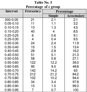
Once we have done this exercise, we proceed to calculate the frequency of the elements that are above and below the reference household (the set of numeral 3c). We repeated the methodology 1000 times and calculated the percentage of households that belonged to group c. If the percentage of households in group c is above 10%, the substitutability condition is approved.
11 This method do not have any assumption on residuals distribution. Residual kurtosis is 60, which is high and
Table No. 5 Percentage of c group
Interval Frecuency Percentage
Simple Accumulate
000-0.05 0.05-0.10 0.10-0.15 0.15-0.20 0.20-0.25 0.25-0.30 0.30-0.35 0.35-0.40 0.40-0.45 0.45-0.50 0.50-0.55 0.55-0.60 0.60-0.65 0.65-0.70 0.70-0.75 0.75-0.80 0.80-0.85 0.85-0.90 0.90-0.95 21 11 13 40 6 4 24 15 28 51 58 122 95 142 212 102 34 15 7 2.1 1.1 1.3 4 0.6 0.4 2.4 1.5 2.8 5.1 5.8 12.2 9.5 14.2 21.2 10.2 3.4 1.5 0.7 2.1 3.2 4.5 8.5 9.1 9.5 11.9 13.4 16.2 21.3 27.1 39.3 48.8 63 84.2 94.4 97.8 99.3 100 Source: ECV-97. Estimated by the autors.
The first column shows the percentage interval of the existence of group c. The second column is the frequency where the set has been found. We observed that in 21 opportunities the participation of group c in the three sets is lower that 5%. The percentage of times where group c occurred is increasing. In 122 cases, the number of households that experienced substitutability are between 55% and 60% of the total households. We can observe that 78% of the values are above 0.50, which is evidence that substitution of living conditions among households is done. (See table 5).
This result is congruent with the idea that households have different necessities and priorities. It reinforces the idea that ILC is not normative, because it doesn’t suppose that the population must have similar living conditions. For example, the index admits the possibility that a household may have higher educative levels than better quality walls.
V Conclusions
Any social policy needs interpersonal comparisons, and we have shown the concepts of well-being and standard of living elaborated by Amartya Sen because these are adequate for building a social policy theory. Sen thinks that the well-being concept and the standard of living concept are associated to what people can be or do. The well-being of one person takes into account the well – being of others (sympathies and antipathies). Standard of living level is not influenced by the well-being of other people. Standard of living level values what a person can do or be, based in the type of life that the agent lives.
The statistical methodology used to calculate ILC permits the valuation of qualitative variables. These variables represent some of the household living conditions that reflect their functionings and capabilities. The fact that our unit of analysis is the household, introduces a limitation in the index, because it can’t gather the specific situations within each family.
ILC is a valuation of household capabilities and functionings, it is not a well – being index. It is a standard of living index because it doesn’t capture in a direct way the sympathies or the antipathies.
An ILC index must fulfill at least one of the following properties: Monotonicity, Concavity, Non-independence of irrelevant alternatives, Informativity and Substitution of living conditions. Some of them can be proved without performing a test. For example, Monotonicity is fulfilled due to the valuations of the coefficients, and the index functional form. Other properties are not as easy to check, for example, concavity.
The tests showed that Monotonicity, Informativity and substitution of life conditions were fulfilled. So we can say that the ILC overcomes the problems that other indexes had. For example, the Poverty Line doesn’t fulfill Monotonicity, which can’t give sufficient information about people’s living conditions. ILC gives more information than the Poverty Line. Substitution is an exclusive property of the composed indexes, so we can say that the index is taking into account the differences between living conditions of households. Living conditions differences are produced by freedom or by restrictions that households confront.
Concavity is a desirable property, but it is difficult to prove it. Continuity can be guaranteed if we use the municipality averages. But, this exercise introduces social judgments. There are other methodological instruments which can be use to prove continuity. For example, we can use the vector space generation procedure, which is used to prove and deal with the continuity problem.
Although ILC index can be use to measure standard of living levels, we have to keep working on its assumptions, and on its applicability.
Our new task will be think into new conditions to construct the ILC index. At first, the objective was to find out how to target the public investment in health programs, but if we understand it as a standard of living index, we enrich its meaning. In future opportunities, other living conditions such as environmental dimensions, political participation, etc, can be introduced to measure the standard of living level index.
References
ACOSTA Rodrigo., 1997. El Indice de Condiciones de Vida Modificado, Master Tesis, Department of Economics, Universidad Nacional. Colombia
ARROW Kenneth., 1951. Social choice and Individual Values, Oxford.
ARROW Kenneth., 1977. “Extended Sympathy and the Possibility of Social Choice”, American Economic Review Papers and Proceedings, 67, pp. 219-225. Reproduced in Collected Papers of Kenneth Arrow. Social Choice and Justice, vol. 1, Cambridge, Mass.: Belknap Press, Harvard University Press, 1983, pp. 147-161.
ARROW Kenneth., HAHN Frank., 1972. General Competitive Analysis, Holden-Day, San Francisco.
CASTAÑO Elkin., MORENO Hernando., 1994. “Selección y Cuantificación de Variables del Sistema de Selección de Beneficiarios, SISBEN”, Planeación & Desarrollo, Vol. XXV, junio, ed. especial.
CHIANG Alpha., 1984. Fundamental methods of mathematical economics, Mc. Graw Hill, third edition,
HAWTHORN Geoffrey., 1987. “Introduction”, en HAWTHORN Geoffrey., ed. The Standard of Living, Cambridge University Press, Cambridge, pp. vii-xiii.
HERNANDEZ Andrés., 1998. “Amartya Sen: Ética y Economía. La Ruptura con el Bienestarismo y la Defensa de un Consecuencialismo Amplio y Pluralista”, Cuadernos de Economía, Vol. XVII, no. 29, segundo semestre, pp. 137-162.
KOOPMANS Tjalling., 1957. Tres Ensayos sobre el Estado de la Ciencia Económica, Antoni Bosch, 1980.
MISION SOCIAL., DEPARTAMENTO NACIONAL DE PLANEACION, DNP., 1998.
Informe de Desarrollo Humano para Colombia 1998, Tercer Mundo, DNP, PNUD.
NUSSBAUM Martha., SEN Amartya., 1993, comp. La Calidad de Vida, Fondo de Cultura Económica, México, 1996.
OVEJERO Félix., 1994. “Las Defensas Morales del Mercado”, Isegoría, no. 9, CSIC, abril, pp. 41-63.
PROGRAMA DE LAS NACIONES UNIDAS PARA EL DESARROLLO, PNUD., 1991.
Desarrollo Humano: Informe 1991, New York.
SARMIENTO Alfredo., RAMIREZ Clara., 1997. El Indice de Calidad de Vida, DNP, Misión Social,
SARMIENTO Alfredo., RAMIREZ Clara., 1998. “Tipología Municipal con Base en las Condiciones de Vida”, en SARMIENTO Libardo., ALVAREZ María., direc. Municipios y Regiones de Colombia. Una Mirada desde la Sociedad Civil, Fundación Social, Federación Colombiana de Municipios, Consejo Nacional de Planeación, pp. 247-262.
SAS/STAT User Guide., 1990. Volume 2, Version 6, Cuarta edición, SAS Institute Inc., Cary, NV, USA.
SEN Amartya., 1970. Collective Choice and social welfare, Oxford, 1976.
SEN Amartya., 1973. On Economic Inequality, Oxford University Press.
SEN Amartya., 1977. “Rational Fools: A Critique of the Behavioral Foundations of Economic Theory”, Philosophy and Public Affairs, summer, 6 (4), pp. 317-344. Reproduced in Choice, Welfare and Measurement, 1982, Harvard University Press, 1997, pp. 84-108.
SEN Amartya., 1985. Commodities and capabilities, North – Holland, Amsterdam
SEN Amartya., 1985b. “Well Being, Agency and Freedom: The Dewey Lectures 1984”, The Journal of Philosophy, Apr., no. 82 (4), pp. 169-221.
SEN Amartya., 1987. On Ethics and Economics, Basil Blackwell, Oxford.
SEN Amartya., 1987. b. “The Standard of Living: Lecture I, Concepts and Critics”, en
HAWTHORN Geoffrey., ed. The Standard of Living, Cambridge University Press, Cambridge, pp. 1-19.
SEN Amartya., 1987. c. “The Standard of Living: Lecture II, Lives and Capabilities”, en
HAWTHORN Geoffrey., ed. The Standard of Living, Cambridge University Press, Cambridge, pp. 20-38.
SEN Amartya., 1990. “Justice: Means versus Freedoms”, Philosophy and Public Affairs, no. 19, pp. 111-121.
SEN Amartya., 1992. Inequality Reexamined, New York: Rusell Sage Foundation; Cambridge: Harvard University Press.
SEN Amartya., 1993. “Markets and Freedoms: Achievements and Limitations of the Market Mechanism in Promoting Individual Freedoms”, Oxford Economic Paper, no. 45, pp. 519-541.
SEN Amartya., 1997. “Maximization and the Act of Choice”, Econometrica, vol. 65, no. 4, july, pp. 745-779.
VELEZ Carlos E., CASTAÑO Elkin., DEUTSCH Ruthanne., 1998. An Economic Interpretation of Colombia’s SISBEN: A composite Welfare Index Derived from The Optimal Scaling Algorithm. Ponencia presentada en Argentina
WILLIAMS Bernard., 1985. Ethics and the Limits of Philosophy, Cambridge MA: Harvard University Press.
WINSBERG S., RAMSAY J.O., 1983. "Monotone Spline Transformations for Dimension reduction", Psychometrika, 48, 575-595.
WOLD H., LITKENS E., 1969. "Nonlinear Iterative Partial Least Squares (NIPALS) Estimation Procedures", Bulletin ISI, 43, 29-47.
YOUNG F.W., 1975. "Methods for Describing Ordinal Data with Cardinal Models", Journal of Mathematical Psychology, 12, 416-436.
YOUNG F.W., TAKANE Y., DE LEEUW J., 1978. "The Principal Components of Mixed Measurement Level Multivariate Data: An Alternating Least Squares Method with Optimal Scaling Features", Psychometrika, 43, 279-281.
YOUNG F.W., TAKANE Y., DE LEEUW J., 1985. "PROC PRINQUAL- Preliminary Specifications", Non published Manuscript, The University of North Carolina Psychometric Laboratory, Chapel Hill NC.