V
IGNETTES AND SELF
-
REPORTED WORK DISABILITY IN
THE
U
NITED
S
TATES
:
C
ORRECTION OF REPORT
HETEROGENEITY
.
A
NDRESF
ELIPEP
ATINOR
EPIZOM
ASTERT
HESISS
UPERVISOR:
D
OLORES DE LAM
ATAU
NIVERSIDAD DELR
OSARIOF
ACULTAD DEE
CONOMÍAMS
C.
E
CONOMICSABSTRACT
SUBJECTIVE MEASURES OF HEALTH TEND TO SUFFER FROM BIAS GIVEN BY REPORTING HETEROGENEITY.
HOWEVER, SOME METHODOLOGIES ARE USED TO CORRECT THE BIAS IN ORDER TO COMPARE SELF-ASSESSED
HEALTH FOR RESPONDENTS WITH DIFFERENT SOCIODEMOGRAPHIC CHARACTERISTICS. ONE OF THE METHODS TO CORRECT THIS IS THEHIERARCHICAL
ORDERED
PROBIT
(
HOPIT
), WHICH INCLUDES RATES OF
VIGNETTES-HYPOTHETICAL INDIVIDUALS WITH A FIXED HEALTH STATE- AND WHERE TWO ASSUMPTIONS
HAVE TO BE FULFILLED, VIGNETTE EQUIVALENCE AND RESPONSE CONSISTENCY. THIS METHODOLOGY IS USED
FOR THE SELF-REPORTED WORK DISABILITY FOR A SAMPLE OF THE UNITED STATES FOR 2011. THE RESULTS SHOW THAT EVEN THOUGH SOCIODEMOGRAPHIC VARIABLES INFLUENCE RATING SCALES, ADJUSTING FOR THIS DOES NOT CHANGE THEIR EFFECT ON WORK DISABILITY, WHICH IS ONLY INFLUENCED BY INCOME.THE
INCLUSION OF VARIABLES RELATED WITH ETHNICITY OR PLACE OF BIRTH DOES NOT INFLUENCE THE TRUE WORK DISABILITY. HOWEVER, WHEN ONLY ONE OF THEM IS EXCLUDED, IT BECOMES SIGNIFICANT AND AFFECTS THE TRUE LEVEL OF WORK DISABILITY AS WELL AS INCOME.B
OGOTÁ,
C
OLOMBIAA
UGUST2012
1
1
Table of Contents
1. Introduction ... 3
2. Literature Review ... 6
3. Data and descriptive statistics ... 8
4. Econometric Methodology ... 12
5. Specification of the Models ... 15
5.1. Ordered Probit Model (without correction) ... 15
5.2. Vignette Component ... 15
5.3. HOPIT Model ... 16
6. Results ... 16
6.1. Ordered Probit Model (without correction) ... 16
6.2. Vignette Component ... 17
6.3. HOPIT Model ... 18
7. Discussion ... 23
8. References ... 26
1. Introduction
Many developed economies experience problems related to reducing work disability and this issue is being placed higher on the policy agenda in order to enhance economic performance. Disability had become an important topic, as approximately one of five people that belong to the working age group is disabled (Smith and Twomey, 2002). This situation is increasing the direct and indirect influence of disability, not just in the labor market but in the whole economy. However, work disability does not affect the whole society in the same proportion as some differences across groups are present: for instance, most of the workers experiencing disability problems have a high age (Banks et al. 2004), but work disability is indifferent to gender.
The situation for the United States does not differ from most other developed countries. Disability insurance recipients between 45 and 64 years old have increased for both genders in the last two decades (Autor and Duggan, 2003; Bound and Burkhauser, 1999; Burkhauser et al., 2008). According to the U.S. Social Security Administration, a 20 year old worker has 30% chance of becoming disabled before reaching the retirement age; it makes work disability something that has to be treated not just in a scientific context, but also in a policy perspective. However, conditions of disabled workers are different across countries; issues such as disability insurance, access to treatment and eligibility rules are addressed in a different way, making this situation hard to compare in quantitative terms.
Comparisons between the United States and other developed countries have been made (Kapteyn et al. 2007) in order to identify differences in work disability across countries and to adopt policies that are successful in other societies. In the other hand, comparisons may also be made across groups within countries, to identify if work disability vary according to sociodemographic factors to evaluate health in terms of equity and equality.
Measurements of health may differ in substantial ways; there are objective measures like the Quality
Adjusted Life Yea s QALY’s , Disa ilit Adjusted Life Yea s DALY’s o the M Maste Health Utilit I de
(HUI-3) and subjective measures, such as self-assessed or self-reported health. The first group reflects a true measure of health using an objective scale, but they are really expensive. The second one proceeds from surveys, but may generate subjective scales, as the answers given by the respondents depend on various factors including age, gender, education, income and ethnicity (see Salomon et al. 2004; Bago
Co pa i g su h self-reports of work disability, account should be taken of measurement issues such as differences in question wordings, justification bias and other reporting biases, as well as differences between and within countries that may exist in the scales that are used in answering questions about
o k disa ility .
In the literature the problem given by reporting heterogeneity receives three names, State-dependent reporting bias (See Kerkhofss and Lindeboom 1995), Scale of reference bias (See Groot 2000) and response category cut-point shift (See Sadana et al. 2000; Murray et al. 2001). The effort to find the real health and correct the bias given by reporting heterogeneity asks for different techniques. One of the methods uses hypothetical fixed levels of health, where differences in the rating can be attributed to differences in reporting behavior. Kapteyn et al. des i e ho the appi g of t ue health i to Self-assessed Health (SAH) categories varies depending on the characteristics of the respondent.
In Kapteyn et al. (2007) the authors use a methodology called anchoring vignettes to adjust for reporting biased and compare the difference between the United States self reports of work disability with the ones from The Netherlands. The results show that the Dutch have lower thresholds for perceived work disability and the correction made using vignettes reduces the gap observed between both countries by 60%. The purpose of this work is to evaluate the difference in self-reported work disability across sociodemographic groups for the United States, correcting the reporting heterogeneity in order to be able to compare work disability. Kapteyn et al. (2007) did this type of research with a set of data from 2003 to 2004, with a comparison between United States and the Netherlands for work disability. This study applies the same methodology for a more recent set of data (January – March of 2011) for United States which is different in some dimensions such as the inclusion of diseases (for instance Kapteyn et al. (2007) include Hypertension, Diabetes, cancer and disease of lung) that are not included in this study. The difference of Work Disability scales for two different individuals is illustrated in Figure 1. represents a low work disability (high health) and a high work disability (low health). L and H are people with different scales, where person L has a lower response cut point and as such, a lower
p o a ilit to ate a fi ed le el of health as o espo di g to ot a le to o k . The se o d pe so , H,
has a higher response cut point, meaning that the probability of rating a fixed level of health as
o espo di g to ot a le to o k ill e highe tha fo pe so L. The s ale a a depe di g o
attributes of the respondents. Better educated people for instance, may rate themselves less disabled than less educated people (see Bago d’U a et al. ; older individuals tend to report less work disability levels because of the shifting norms for health over the life course (see Salomon et al. 2004) and this may occur for other sociodemographic factors such as gender, income and ethnicity. Although we can see that represents a lower work disability than , the difference between both self-reported health states can also be generated because of different response cut-points.
generalization receives the name of Hierarchical Ordered Probit (HOPIT) given by Tandon et al. (2003) and King et al. (2004). This model is the combination of two models and allows heterogeneous cut-points on the model for self-assessed work disability. The first model involves making the cut-points dependent on the exogenous variables and the vignettes. The second model encompasses the inclusion of these variable cut-points in the estimation for the self-assessed work disability. It makes possible to differentiate between reporting behavior and own health. However, two assumptions have to be fulfilled, vignette equivalence and response consistency (King et al. 2004). The first assumption implies that the vignette description is perceived by all respondents to correspond to the same health state. The second one states that individuals use the same response scales to rate the vignettes and their own situation. A vignette question describes the health of a hypothetical person and then asks the
espo de t to e aluate that pe so ’s health o the sa e s ale used fo a self-report on their own health.
Usi g the fi st assu ptio , e k o that the t ue health state fo a ig ette is o sta t a d it ill e
This work proceeds as follows. Section 2 provides a literature review on the use of anchoring vignettes. Section 3 outlines the data and the descriptive statistics, including the vignettes used. Section 4 presents the econometric methodology. Section 5 outlines the specification of the models that are developed. Section 6 provides an analysis of the results. Section 7 outlines the discussion that covers the conclusions and extensions. References and Appendix are in Section 8 and 9 respectively.
2. Literature Review
The use of anchoring vignettes in social sciences has grown considerably in the last few years. The methodology proposed by King et al. (2004) to correct for differences in the response scales (DIF,
diffe e tial ite fu tio i g ) has been used not only in the field of health but also in politics,
In the field of health economics, Salomon et al. (2004) examines the differences in self reported health rates, due to expectations for health states (expected self rating of health) using 15 anchoring vignettes for mobility, in China, Turkey, United Arab Emirates and others. They computed rank correlations for the individual vignette ratings but they do not formally test the vignette assumptions (vignette equivalence and response consistency). The comparison of vignette rankings let them support the idea that respondents have different health expectations, which generate different ratings (for instance, ratings for vignettes declines with age in the dimension of mobility). In the other hand, response consistency is supported by the comparison between self rates and rates for vignettes in two questions, where the same respondents use the categories similarly in rating themselves and the vignettes. As a conclusion, they emphasize that vignettes are a useful instrument for understanding and adjusting the influence of different health expectations on self ratings of health. Murray et al. (2003) use health to evaluate the vignette approach in the domain of mobility. The sample was composed of 55 countries from the Multi-Country Survey Study (WHO-MCS, 2000–2001). The results show that age, gender and education may change the scales of the report of health as a consequence of cross-country differences.
Other articles use the vignettes methodology to test the differences in health reporting by educational level. Bago d’U a et al. (2008), check the effect of the educational level in the bias on the measurement of health inequalities using data from SHARE (Survey of Health, Ageing and Retirement in Europe) for eight countries, using six domains (mobility, pain, sleep, breathing, emotional health and cognition), where the differences in the scale rate are corrected using a HOPIT model. Before the correction there was no inequality in health by education in most of the cases (32 of 48). The correction increases health inequalities in most of the cases.
Subjective health reports may be highly related with own opinions about health, for instance someone who suffers from a disease since a long time ago may rate himself better than someone healthier that suffers recently from a minor disease. This also may occur when vignettes are rated; their health state rating may be different if the person who is rating is completely healthy or if it is someone with some health limitations. Salomon et al. , uses the se te e you know it when you see it to efe to this issue, and i di iduals u de sta d the same uestio i astly diffe e t ays to describe the problems that the heterogeneity generate in terms of comparisons between two different sociodemographic groups.
showed in a medical test). Slovakia had less vision problems than China, but the difference in scales lead to a similar self-reported vision level in both countries. The correction using vignettes gives an answer in the same direction than a medical test and supports that even if vignettes do not solve all the problems, they have the potential to reduce biases in the comparisons.
It is common to identify differences in reports between sub-groups, for instance between men and women or old and young people. This indicates that health state has different thresholds due to socio economic factors rather than true differences in work disability. This is the reason why some articles use a more objective indicator of health, like the McMaster Health Utility Index (HUI-3). For example, Lindeboom and van Doorslaer (2004) find cut-points shifts for age and gender but not for income or education.
The use of vignettes has some limitations, because they do not necessarily correct the differences as in some cases the results of the corrections are contradictory. I Bago d’U a et al. (2011), corrections in the domains (cognitive functioning and physical functioning) were not successful in terms of increasing the correlation between self-assessed health and an objective measure such as the given by the English Longitudinal Study of Ageing (ELSA) cognitive function module. Furthermore, corrections of scales in the domain of cognition did not seem to be successful but corrections of scales in mobility appeared to reduce the differences given by heterogeneity.
When comparing two developed economies such as the United States and the Netherlands Kapteyn et al. (2007) found that without any heterogeneity correction for an age group between 51 and 64, the American self-reported work disability is 22.7% where the Dutch report indicates self-reported work disability is 35.8%. Correcting the response scales using the vignettes methodology, if both countries are compared with the American scale, the Dutch report is just 28.3%, which means that more than half of the difference in the work disability rates is caused by a different response scale. The data comes from the Dutch CentER panel for 2003, the RAND MS (monthly survey) for 2004 and the Health and Retirement Study in 1998.
3. Data and descriptive statistics
The age of individuals in the sample2 goes between 22 and 92 years, but most of the sample (more than 90% of the sample) is between 45 and 80 years with an average of 59 years. Males represent 45% of the sample.
Education is measured using three dummies: Low Education, that starts from 7th or 8th degree to some college but no degree (less than 10 years of education); Middle Education, which starts from associate degree in college to bachelor’s degree (11-13 years of education); and High Education, that starts from master’s degree to doctorate degree (14-16). The omitted category is Low Education.
The last group of variables is related with income Low Income takes the value 1 if the income is $39,999 or less and 0 otherwise; Middle Income takes the value of 1 if income is between 40,000 and 75,000 and 0 otherwise; and High Income is 1 if income is more than $75,000, and 0 otherwise. These variables are constructed from a variable called Family Income, which is a qualitative variable that classifies income in 14 categories depending on the range of the income of the family. The purpose of the income transformation was to have three representative income groups, with approximately the same proportion of individuals. Additionally, the creation of 3 income groups makes the results more intuitive. A 26.8% of the sample belongs to the low income group, 34.7% to the middle income group and 38.5% to the high income group. For more details about the variables, see Appendix B.
The respondents were asked to rate the work disability for 5 vignettes in 3 domains, namely cardiovascular disease (CVD), affect (depression) and pain using the same response categories than in the self-assessed work disability. The gender of the 15 vignettes was selected randomly. The wording of all the vignettes questions is: Does M /M s X ha e a y i pai e t o health p o le that li its the ki d
o a ou t of o k you that he/she a do? .
2
[image:9.612.84.536.357.575.2]Two variables were included for age in the model, the first one is age divided by 100 (age/100) and that variable squared ((age/100)squared). The reason was to include the same age variables than Kapteyn et al. (2007).
Table 1
Description Mean Standard Deviation Self Assessed Work Disability WD Categorical (1-5) 1.5506 0.9894
Highest Education Level HEL Categorical (4-16) 11.865 2.0305
Low Education LE Dummy 0.3681 0.4827
Middle Education ME Dummy 0.3880 0.4877
High Education HE Dummy 0.2439 0.4297
Male M Dummy 0.4463 0.4975
Age A & SA Discrete 58.538 10.675
White W Dummy 0.9172 0.2758
Income I Categorical (1-14) 11.520 2.9948
Low Income LI Dummy 0.2684 0.4435
Middle Income MI Dummy 0.3466 0.4763
High Income HI Dummy 0.3850 0.4870
In order to a al ze the ati gs of the ig ettes o ditio al o i di idual’s ha a te isti s, I fi st do a descriptive analysis conditioning in two sociodemographic variables: education and ethnicity. To do the analysis it is worth remembering that according to the vignette equivalence assumption, all the vignettes have a fixed work disability level. Hence, observed differences in ratings for different education groups, or ethnicity, may indicate the presence of heterogeneity and different rating scales. For more details about the vignettes description, see Appendix C.
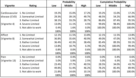
Table 2 presents the work disability rates given by individuals with different levels of education and the cumulative probabilities for 3 vignettes (1 per domain), that are chosen randomly. The Cardiovascular
Disease CVD ig ette is ated as athe li ited for the majority of the low-education group (38.08%),
ut the ost popula ate is so e hat li ited fo the iddle a d high-education groups (39.13% and 49.68% respectively). For the affect vignette, most of the middle-educated individuals rate the work disa ilit situatio as athe li ited , he eas i the majority of low and high-educated individuals rate
thei o k disa ilit as so e hat li ited . Additio all , the pe e tage of lo -educated individuals who rate that vignette into the two worst catego ies se e e li ited a d ot a le to o k is o e than two times than that of high-educated individuals.
Something similar happens with the pain vignette, where differences between low-education and high-education are larger. People with a low-educatio , ho ated the ig ette as ot a le to o k (21.76%) are proportionally two times larger than the percentage of the vignette from high-income
people ho ga e the sa e a s e . % . The opposite happe s ith the athe li ited atego ,
Performing the same analysis for ethnicity (Table 3), we can see that both groups tend to give similar rates to the three vignettes. The proportion of non- hite people that gi e the t o o st states se e e
li ited a d ot a le to o k to the ig ette is, ho e er, larger than the proportion of white people. Furthermore, white people tend to give a better rate (healthier) to the CVD vignette than non-white people. The rates for the other two vignettes (affect and pain) however, are quite similar, excluding the cases of athe li ited a d ot a le to o k i the pai ig ette, he e diffe e es et ee athe
li ited a d ot a le to o k a e al ost dou le fo oth g oups.
Analyzing the cumulative probabilities for the pain vignette, we can see that non-white people have a
highe p o a ilit to ate the ig ettes i to the t o fi st g oups o li ited a d so e hat li ited
[image:11.612.71.545.97.371.2]than white people. However, it is the opposite in the third and fourth state, where most of the white individuals rate the vignette in that state (80%) and a less proportion of non-white gave that rate (60%). Tables 2 and 3 reflect that there may be an influence of sociodemographic variables in health perception. The rates for similar states of health differ between educational levels and between ethnicity supporting the presence of differences in rating scales for different respondents. However, we do not know if these differences are only due to differences in scales or if these sociodemographic variables are also influencing the true work disability. To provide corrections, tables are not enough and econometric methodologies such as the HOPIT specification have to be used.
Table 2
Descriptive of Vignettes by Highest Education Level
Vignette Rating Low Middle High Low Middle High
Cardiovascular 1. No Limited 19.2% 15.0% 17.2% 19.2% 15.0% 17.2% disease (CVD) 2. Somewhat Limited 29.3% 39.1% 49.7% 48.5% 54.2% 66.9% 3. Rather Limited 38.1% 33.2% 28.7% 86.6% 87.4% 95.5% (Vignette 4) 4. Severe Limited 13.0% 11.1% 4.5% 99.6% 98.4% 100.0% 5. Not able to work 0.4% 1.6% 0.0% 100.0% 100.0% 100.0%
100% 100% 100%
Affect 1. No Limited 12.1% 11.5% 13.8% 12.1% 11.5% 13.8%
(Vignette 8) 2. Somewhat Limited 36.8% 35.6% 40.9% 49.0% 47.0% 54.7% 3. Rather Limited 36.4% 42.3% 38.4% 85.4% 89.3% 93.1% 4. Severe Limited 13.8% 10.7% 6.3% 99.2% 100.0% 99.4% 5. Not able to work 0.8% 0.0% 0.6% 100.0% 100.0% 100.0%
100% 100% 100%
Pain 1. No Limited 0.0% 0.4% 0.6% 0.0% 0.4% 0.6%
(Vignette 13) 2. Somewhat Limited 5.0% 5.9% 2.5% 5.0% 6.3% 3.2% 3. Rather Limited 23.4% 27.7% 40.5% 28.5% 34.0% 43.7% 4. Severe Limited 49.8% 51.4% 46.2% 78.2% 85.4% 89.9% 5. Not able to work 21.8% 14.6% 10.1% 100.0% 100.0% 100.0%
100% 100% 100%
4. Econometric Methodology
The purpose of this work is to estimate the effect of sociodemographic variables on work disability. In order to do this, models will have to be performed. However, some of them may suffer from reporting heterogeneity and because of that, various corrections will have to be carried out. The first part presents the relation between self-assessed work disability and sociodemographic variables in an Ordered Probit model.
Where is the latent level of work disability of respondent , is a vector of covariates (including a constant term), is the error term and represents the thresholds for the five categories of work disability ( is equal for all the respondents).
[image:12.612.96.518.80.357.2]However, this model has the assumption of homogeneous reporting behavior. If there is heterogeneity in reporting, these cut-points will not reflect the real reporting scale, because they are fixed and there is no interaction between them and the sociodemographic variables. It may also cause the estimated coefficients to be biased, because they will capture real work disability effects but also reporting effects. These heterogeneity problems can be corrected using the vignettes model, which allows the cut-points to depend on the sociodemographic variables, and estimate (using the adjusted cut-points) the true effect on work disability.
Table 3
Vignette Rating Non White White Non White White
CVD 1. No Limited 16.7% 17.1% 16.7% 17.1%
(Vignette 4) 2. Somewhat Limited 29.6% 38.8% 46.3% 56.0%
3. Rather Limited 35.2% 33.8% 81.5% 89.7%
4. Severe Limited 16.7% 9.6% 98.1% 99.3%
5. Not able to work 1.9% 0.7% 100.0% 100.0%
Affect 1. No Limited 14.8% 12.1% 14.8% 12.1%
(Vignette 8) 2. Somewhat Limited 29.6% 38.0% 44.4% 50.1%
3. Rather Limited 37.0% 39.4% 81.5% 89.4%
4. Severe Limited 13.0% 10.6% 94.4% 100.0%
5. Not able to work 5.6% 0.0% 100.0% 100.0%
Pain 1. No Limited 1.9% 0.2% 1.9% 0.2%
(Vignette 13) 2. Somewhat Limited 7.4% 4.5% 9.3% 4.7%
3. Rather Limited 14.8% 30.5% 24.1% 35.2%
4. Severe Limited 46.3% 49.8% 70.4% 85.1%
5. Not able to work 29.6% 14.9% 100.0% 100.0%
Descriptive of Vignettes by Ethnicity
The vignettes are hypothetical cases that represent fixed levels of health; under the assumption of vignette equivalence, variation in vignette ratings can only be generated by reporting heterogeneity or DIF (differential item functioning). Furthermore, a generalization of the Ordered Probit can be performed using the vignettes, in which the cut-points are allowed to vary with individual characteristics. This generalization receives the name of Hierarchical Ordered Probit (HOPIT) given by Tandon et al. (2003) and King et al. (2004). This model is a one-step estimation that includes the estimation of the self-assessed work disability model and the estimation of the cut-points depending of the socio economic variables exploiting the vignettes information. It allows heterogeneous cut-points on the model for self-assessed work disability, making it possible to disentangle the effect of socioeconomic variables on the true work disability from the effect these variables have on reporting behavior. The HOPIT model can be understood as a full model, with one vignette component, that uses the vignettes to identify the cut-points and a second component where the cut-points are imposed to correct the reporting problem, obtaining the effect of socioeconomic variables on the true work disability.
The first part is a vignette component and can be described as a Generalized Ordered Probit for the vignette ratings, given by:
Where is the latent level of work disability of vignette perceived by respondent , are the health characteristics of vignette described in the Appendix C, is the error term and the total number of vignettes is 15 in this application. The latent level of work disability of vignette is mapped into the reported category of work disability in the following way:
where . The cut-points can depend on covariates or can be fixed in order to compare specifications:
or
where is a vector of constant terms that can be the same for all the cut-points or not.
To model heterogeneity, covariates are only included in the cut-points. In other words, when the vignette equivalence assumption holds, variation in vignette work disability can only be attributed to reporting behavior.
The probabilities for all the categories for a given vignette are specified by:
where is the cumulative standard normal distribution, and j increases with a higher work disability level.
on the true own work disability. If assumptions hold (vignette equivalence and response consistency) the model is identified and the latent level of work disability of the respondent is equal to:
where is a vector of covariates (including a constant term). The observed categorical variable is related to as follows:
where is: .
Every cut-point is obtained in the reporting behavior model and is included with the coefficients and the standard deviation in the estimation of self-reported work disability. It is assumed that:
In other words the work disability level of the vignette will be independent of the work disability level of the respondent for all the respondents and all the vignettes, meaning that differences in work disability for a vignette can only correspond to different rating scales between respondents. If this assumption does not hold, reporting problems cannot be corrected, because differences in perceived work disability for a vignette can be caused by differences in own work disability. The probabilities associated with the categories in the true work disability level, will be given by:
where is the cumulative standard normal distribution.
These probabilities enter into the log-likelihood function for the HOPIT model, composed by the sum of log-likelihoods of the two components (vignettes component and own work disability component). According to King et al. (2004) the use of anchoring vignettes to measure diffe e tial ite fu tio i g (DIF) can be represented in the context of work disability (Wd) as a process3, where:
1. If model assumptions hold:
Self assessment work disability estimate: (Wd + DIF)
Vignettes estimate: DIF
Vignette corrected self assessment: (Wd + DIF) - DIF = Wd 2. If model assumptions do not hold:
Self assessment work disability: (Wd + DIFs)
Vignettes estimate: DIFv
Vignette corrected self assessment: (Wd + DIFs) – DIFv = Wd + (DIFs – DIFv)
where DIFs is the self-assessment bias and (DIFs – DIFv) is a Vignette corrected self assessment bias. Usually the second bias is smaller than the first one. In other words, methodologies that correct reporting bias such as the HOPIT, which includes the use of vignettes, are useful even if the assumptions do not hold, because the DIF is reduced. When the assumptions hold, the methodology is able to purge the heterogeneity in reports in a complete way. Furthermore, if the assumptions do not hold, the DIF cannot be completely removed but can be reduced, obtaining results that are closer to the ones with no heterogeneity.
5. Specification of the Models
We organize the empirical specification in the following way. First we estimate the relationship between sociodemographic variables and work disability using a simple Ordered Probit Model, where the results may be biased by heterogeneous reporting behavior. We then formulate a simplified model of reporting behavior, the vignette component, in which it is assumed that the sociodemographic variables affect all the cut-points by the same magnitude4, where the dependent variable is the vignettes rating. Finally, two specifications of the HOPIT model will be presented, one without any correction (only to be compared with the corrected) and a HOPIT that allows the dependence of the cut-points on sociodemographic variables.
5.1. Ordered Probit Model (without correction)
We first estimate the model specified in equation 4.1. The purpose of this model is to find if there is a significant effect between the self-reported work disability and the variables used by Kapteyn et al. (2007) for the new data set (RAND MS-2011).5 In a first specification is a vector of the following sociodemographic characteristics: an indicator of medium education (ME), an indicator of high education (HE), gender (M) and age. Age is included using the same two variables included by Kapteyn et al. (2007) to take into account the non-linear effect of age on Work Disability: which is the age divided by 100 and which is the squared of . The cut-points are fixed and do not depend of the sociodemographic characteristics of the respondents.
In a second specification we consider a more complete set of covariates. The new variables included in this specification, are an indicator that takes the value 1 if the individual is white (W), and two indicators of income, one that indicates whether individual has medium income (M1) or high income (M2), being low income the base category.
5.2. Vignette Component
The two models presented in the sub-section 5.1, have the assumption of homogeneous reporting behavior. If there is heterogeneity in reporting, the cut-points will not reflect the real reporting scale, because they are fixed and there is no interaction between them and the sociodemographic variables. It
4
This specification is not included in the section 4.
5
may also cause the estimated coefficients to be biased, because they will reveal work disability effects and besides that, also reporting effects.
As a first step to analyze the presence of heterogeneous reporting behavior, we estimate models for the vignette component alone, as those presented in equation 4.2. The 15 vignettes ratings are compiled in a single variable, called , and this transformation implies that for every respondent there will be 15 observations, one for each vignette. All specifications include vignettes fixed effects and assume that variables in affect all cut-points in the same magnitude (parallel cut point shift) The vignettes model is estimated by means of a standard Ordered Probit of the variable , depending on the control variables and a variable:
Where is a vector of vignette fixed effects ) 5.3. HOPIT Model
The HOPIT model was explained in the previous section and it is a one-step estimation that includes the estimation of the self-assessed work disability and the estimation of the cut-points depending of the socio economic variables. As stated before, the estimation is made by maximum likelihood and the log-likelihood is a result of two components, the own health (regression of including cut-points) and the vignette component ( depending on the corresponding vignette in a Generalized Ordered Probit for the 15 vignettes with cut-points). For this model, equations (4.2) to (4.9) from the previous sections are estimated.
There are two possible specifications of the HOPIT model, one that imposes constant cut-points (is not corrected for response heterogeneity) and other where cut-points that are allowed to depend of the sociodemographic variables. The only difference between these specifications is the variance of the latent work disability, which makes coefficients not directly comparable across models.
6. Results
6.1. Ordered Probit Model (without correction)
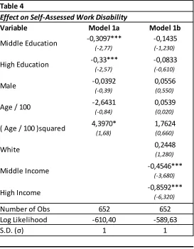
Table 4 reports the Ordered Probit estimates of model specified in equation (4.1). In the first specification (column 1) only the variables related with education are significant. For age, only the squared term is significant and it may indicate that the relation between self-assessed work disability and age is non-linear. Older individuals, for instance, tend to report higher work disability because they feel older and tend to feel less healthy than younger workers. However, the sign of the coefficient of the linear effect of age is negative (but not significant).
The second specification (column 2) also includes income and ethnicity. The results show that none of the variables included in the first model are now significant. However, the sign of education remain. The effect of the variable Male is positive but not significant, and age is not significant. Furthermore, the ethnicity is not significant but positive, meaning that white people tend to report a worse work disability level. Regarding the effect of income in the specification, we can see that it is negative and significant.
The comparison between the two models allows us to point out three interesting things. The first, is that for these two models almost no variable is significant and only the effect of education and income is significant, which may indicate that the variables affect both, the true own work disability as well as the scale, in a sense that both of them move in the same direction. That is to say, the result of the reported own work disability remains the same independent of the sociodemographic variables. The second point is that Model 1b fits the data better, because it has less negative log likelihood (-589.63). Third, given that income is endogenous, the negative correlation between income and work disability cold be just explained by the fact that poor individuals have biased perceptions about their own health and not because they have worst health status.
[image:17.612.171.444.158.509.2]6.2. Vignette Component
Table 4
Variable Model 1a Model 1b
-0,3097*** -0,1435
(-2,77) (-1,230)
-0,33*** -0,0833
(-2,57) (-0,610)
-0,0392 0,0556
(-0,39) (0,550)
-2,6431 0,0539
(-0,84) (0,020)
4,3970* 1,7624
(1,68) (0,660)
0,2448
(1,280)
-0,4546***
(-3,680)
-0,8592***
(-6,320)
Number of Obs 652 652
Log Likelihood -610,40 -589,63
“.D. σ 1 1
Effect on Self-Assessed Work Disability
Middle Education High Education Male
Age / 100
Note: Standard errors in parenthesis. *, ** and *** indicate significance at 10 pecent, 5 percent and 1 percent respectively. ( Age / 100 )squared
White
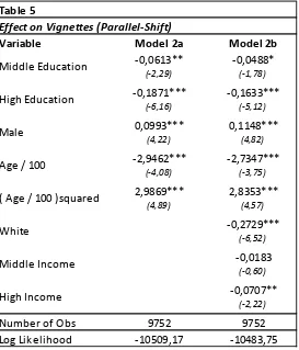
Table 5 reports the Ordered Probit model for the effect of socioeconomic variables on perceptions about situations described in vignettes. In both specifications all the variables are significant (except middle income) and hold the same sign, meaning that under the parallel-shift assumption all the variables influence the scale that respondents give to the vignettes.
Negative coefficients for education (middle and high), income (middle and high) and white mean that respondents that belong to any of these groups are less likely to give higher ratings to the vignettes. For instance, people with a higher education place their cut-points higher, which mean that the probability that they will rate themselves with a lower work disability is high. On the other hand, Males are more likely to place themselves in higher levels of work disability is higher.
In the second specification, the middle income group is not significant, but is negative, just as the high income. The models of Table 5 assume that the cut-point shift is parallel. However if reporting heterogeneity is stronger at some levels of work disability than in others, changes in the cut-point are not the same. This explains why the HOPIT models are relevant in this context, because it allows for a different magnitude in relation between sociodemographic factors and the cut-points.
6.3. HOPIT Model
[image:18.612.172.445.142.461.2]Given that previous results show clear symptoms of reporting heterogeneity, the next step is to correct it using the HOPIT specification in which the cut-points are allowed to vary. Table 6 reports the estimates of the HOPIT with fixed cut-points (column 2) and with cut points that depends on covariates (column 3).
Table 5
Variable Model 2a Model 2b
-0,0613** -0,0488*
(-2,29) (-1,78)
-0,1871*** -0,1633***
(-6,16) (-5,12)
0,0993*** 0,1148***
(4,22) (4,82)
-2,9462*** -2,7347***
(-4,08) (-3,75)
2,9869*** 2,8353***
(4,89) (4,57)
-0,2729***
(-6,52)
-0,0183
(-0,60)
-0,0707**
(-2,22)
Number of Obs 9752 9752
Log Likelihood -10509,17 -10483,75
( Age / 100 )squared White
Middle Income High Income
Effect on Vignettes (Parallel-Shift)
Middle Education High Education Male
[image:19.612.79.720.156.473.2]
19
Table 6
Variable
(1) -0,1435 (2) -0,3098 (3) -0,3143 (4) -0,0354 (5) 0,0427 (6) 0,0502 (7) 0,1475***
(-1,230) (-1,27) (-1,27) (-0,77) (1,14) (1,3) (2,79)
-0,0833 -0,2091 -0,1562 0,0061 0,1090** 0,2080*** 0,4702***
(-0,610) (-0,73) (-0,540) (0,12) (2,51) (4,57) (6,86)
0,0556 0,1381 -0,0015 -0,1501*** -0,1241*** -0,10560*** -0,0649
(0,550) (0,64) (-0,01) (-3,77) (-3,81) (-3,13) (-1,350)
0,0539 0,4069 1,8933 1,2094 3,1599*** 3,4239*** 3,0768**
(0,020) (0,06) (0,27) (1) (3,16) (3,34) (2,26)
1,7624 3,2165 1,2938 -1,7584* -3,3778*** -3,3657*** -2,6259**
(0,660) (0,57) (0,23) (-1,70) (-3,98) (-3,86) (-2,26)
0,2448 0,5081 0,6825* 0,1402** 0,2063*** 0,258*** 0,5151***
(1,280) (1,25) (1,66) (1,98) (3,59) (4,43) (7,08)
-0,4546*** -0,9891*** -0,9651*** 0,0307 0,0125 0,0001 0,0048
(-3,680) (-3,8) (-3,66) (0,6) (0,3) (0) (0,08)
-0,8592*** -1,8093*** -1,7317*** 0,0943* 0,0599 0,0277 0,1144*
(-6,320) (-6,16) (-5,82) (1,77) (1,38) (0,62) (1,79)
-0,1284*** -0,4487*** 1,4949*** 2,0828*** 2,8983*** 3,8028***
(-0,06) (-0,21) (4,11) (6,84) (9,28) (9,38)
Number of Obs. 652 652 652
Log Likelihood -589,63 -11175,20 -11053,02
“.D. σ 1 2,1045*** 2,1117***
(Influence of variables on the cut-points)
Age / 100
Effects of sociodemographic variables on Self-reported Work Disability and Cut points for ALL THE MODELS
Middle Education
High Education
Male
Ordered Probit Model (Without correction)
HOPIT (Fixed cut-points)
HOPIT (Vignettes Correction)
Cut Point 1 Cut Point 2 Cut Point 3 Cut Point 4
652 ( Age / 100 )squared
White
Middle Income
High Income
The table also includes the influence of the variables on the cut-points (equation 4.4), which is the reporting behavior part of the HOPIT estimation (columns 4 to 7). The first column of table 6 also reports the results of the ordered probit without any correction.
Comparing the three models of self-reported work disability we see that the effect of the explanatory variables goes in the same direction for most of the variables. Ethnicity (White) is the only variable that became significant after the correction (column 3). The correction does not cause significant changes in the signs of the coefficients and the significance of the variables. For instance, richer people still tend to report a lower self-assessed work disability (higher health level) in average, compared to people with a low income level. Additionally, the largest difference between the three models is the effect of ethnicity that became significant in the HOPIT model that corrects reporting heterogeneity.
In the three last specifications, the effect of age is always positive (but not significant), thereby reducing the probability of reporting a better state of health. However, age does not influence the lowest level of health. The same occurs in Murray et al. (2003). Furthermore, the effect of age in the self-assessed work disability and in the parallel-shift model is quadratic, but it is not easy to see if it is positive or negative because both of the coefficients related with age in the models had different signs. The effect of age will be positive or negative depending of the magnitude. Figure 2 shows the effect of age for three models. In the vignettes model the negative effect is always larger than the positive effect for all ages. Additionally, for the HOPIT specifications, the effect of age is always positive, which means that older people tend to report higher work disability.
We can propose that the scale is influenced by the heterogeneity caused by ethnicity. For instance, white people use a different rating scale than non-white people. Furthermore, this variable influences the true level of work disability for the last specification (column 3), as most of white people obtain safer jobs than non-white people, meaning that white people have, on average, less probability of being disabled or being in the higher states of work disability.
Nevertheless, we cannot forget that in some cases heterogeneity may not be fully corrected, even after the vignette correction, because in some cases heterogeneity can still be present in the sample if the two assumptions of the model are not fulfilled. However, the use of the vignettes may help in the reduction of the bias produced by heterogeneity. King et al. (2004) argue that the bias generated by the correction is less than the bias given by the self-assessment. The table shows that even if most of the variables influence the cut-points, only the variables related with income and white influence the reported work disability. Furthermore, these income variables cause a small effect on the cut-points, meaning that differences in reported work disability given by income only represent true work disability differences. Besides that, differences given by the other variables only influence the rating scale.
does not correct heterogeneity (effect on self-reported work disability is cut off by effect on reporting behavior).
For all the variables (excluding gender) the effect on the cut-points is positive, which means that richer people, white people and more educated people tend to shift upwards the cut-points. This means that for a given true level of work disability, these groups of people report less work disability than people with low income or not white. Although from these variables, only age and ethnicity have a significant effect on all the cut-points. After the correction however, age is not significant in the determination of the self-assessed work disability.
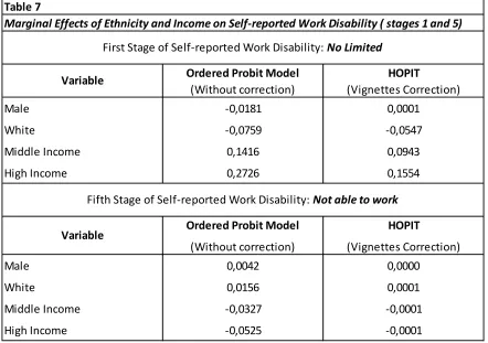
Furthermore, we can analyze if the correction is successful by the use of a marginal effects analysis. To do this, we check the marginal effects of all the variables on the fifth stages of self-reported work disability6: 1. No, not at all, 2. Yes, I am somewhat limited, 3. Yes,I am rather limited, 4. Yes, I am severely limited, 5. Yes, I am very severely limited – I am not able to work. Table 7 shows the marginal effects on
6
the Ordered Probit Model without correction and on the HOPIT model with variable cut-points for the variables were the correction of reporting heterogeneity results in highest differences in marginal effects in the lowest and the highest work disability levels (1. no limited and5. not able to work). These variables are gender, ethnicity, middle income and high income.
For the Ordered Probit specification presented in the second column of Table 7, Male and White have a marginal effect with the same sign (negative in the first stage and positive in the fifth stage), meaning that being male or white decreases the probability of report the lowest work disability level and increases the probability of report the highest work disability level. Something similar occurs with middle income and high income. However the sign of the marginal effects of these two variables is the opposite than the sign of the marginal effect for male and white. For instance, being in the high income category increases the probability of being in the lowest work disability stage in 27.26 percentage points and decreases the probability of being in the highest work disability stage in 5.25 percentage points.
[image:22.612.86.528.412.723.2]In the other hand the HOPIT specification presented in the third column of Table 7, show several differences with the Ordered Probit specification. In the first place all the marginal effects for all the variables are less strong for the HOPIT specification and in the second place Male has the opposite sign for the lowest level of work disability. Additionally we can see that Male, White, Middle Income and High Income have a null marginal effect. However, White, Middle Income and High Income have a marginal effect higher than 5 percentage points on the lowest work disability level. For instance being in the highest income category increases the probability of report the lowest work disability level in 15.54 percentage points.
Table 7
Ordered Probit Model HOPIT
(Without correction) (Vignettes Correction)
Male -0,0181 0,0001
White -0,0759 -0,0547
Middle Income 0,1416 0,0943
High Income 0,2726 0,1554
Ordered Probit Model HOPIT
(Without correction) (Vignettes Correction)
Male 0,0042 0,0000
White 0,0156 0,0001
Middle Income -0,0327 -0,0001
High Income -0,0525 -0,0001
Variable
Variable
Fifth Stage of Self-reported Work Disability: Not able to work
Marginal Effects of Ethnicity and Income on Self-reported Work Disability ( stages 1 and 5)
Bago d’U a et al., (2011) illustrate that the use of vignettes may cause contradictory results; because the cut-points shifts in different directions, meaning that response consistency does not hold. The effects of Middle education and Middle income have a different sign for these two stages. Middle education shifts down the first cut point, but causes an increase in the other cut-points. In the other hand, age and gender shift three of the four cut-points, in comparison to income, which does not shift the cut-points, (income variables are almost not significant in the first and in the fourth one).The same results are found by Lindeboom and van Doorslaer (2004). However, the effect of education is also strong in the cut-points; high education shifts all the cut-points upwards and generates an increase in the probability of reporting worse health. Excluding middle income, the effect of the variables has the same direction for all the cut-points. Gender for instance, is the only variable that moves the cut-points downwards; increasing the probability of reporting higher work disability, but at the end it is not significant in the corrected model.
7. Discussion
Policy related with work disability is growing in importance. In the case of the United States, a dynamic perspective that evaluates benefits and employment rates, generated by Disability Insurance must be carried out. In the last two decades it has been shown that reported rates of work disability considerably influence determinants of employment in posterior periods for industrialized countries (Autor et al., 2003; Bound et al., 1999). The good interaction between the labor market and the disability insurance through policies can generate an increase in the employment rate and a general increase in well-being. (Burkhauser et al., 2008; Coe et al., 2010). However, studies that take a subjective measure such as the self-assessed work disability into consideration should include a correction of the reporting heterogeneity if the goal of the study is to compare ratings for respondents with different sociodemographic characteristics. (King et al. 2004)
The use of vignettes is a good approach to reduce the heterogeneity given by subjective measures of work disability. However, the two basic assumptions of the vignettes methodology (vignette equivalence and response consistency a ot hold fo all ig ettes Bago d’U a et al. 2011; Vonkova et al. 2011). For a data set of the United States in 2011, I find that the effect of income influences the self work disability before the correction and after the correction. Furthermore, the only variables that become significant after the correction is ethnicity.
Regarding age, gender and education, all of these variables affect the standards used to rate self work disability. However, even when the correction makes that these variables influence the scales, the corrected specification (HOPIT with variable cut-points) is not affected by these variables. However, the correction does make a difference for age, gender or education. In the model that corrects reporting heterogeneity, the marginal effects are reduced on the lower and higher work disability levels and increases for levels 2, 3 and 4. Meaning that if the heterogeneity in the reports is not corrected, there is an overestimation of the effect of the variables on work disa ilit i the oute ost health le els o
o k disa ilit a d u a le to o k a d a u de esti atio of these a ia les o the e t al le els
Marginal effects for male, are consistently different for the uncorrected specification (HOPIT with fixed cut-points) and the corrected one (HOPIT with variable cut-points), where the probability of reporting the lowest work disability level is lower for males in the uncorrected specification but is higher for the corrected one.
It is shown in all the specifications that richer people tend to report lower work disability levels. However it can be an effect of endogeneity problems. For instance the relation between work disability and income is bidirectional, meaning that income may affect work disability but it can be also affected by it. For the corrected specification, belonging to the highest income level increases the probability of o
o k disa ilit i . pe e tage poi ts which is lower than the effect for the uncorrected specification (27.26 percentage points). Meaning that the negative effect of income on work disability is lower after the correction of reporting behavior. In other words, if the heterogeneity in the report is not corrected, the effect of income will be overestimated.
In general, after the correction, marginal effects are different than the ones from the uncorrected specification for most of the variables. It may indicate that the correction is useful to measure the real effect on the true work disability and after the correction reporting heterogeneity is purged or reduced. The effect of White is positive for the HOPIT specification (5.3b), it means that white individuals tend to rate themselves with a higher work disability. However, after the marginal effect analysis, we can see that even though being white decreases the probability of being healthier in 5.47%, the probability increases for the intermediate stages of health (1, 2 and 3) and it is close to 0% for the lowest health state, which is supported in the literature, because in most of the cases ethnic minorities (in this case non-white individuals) tend to have a larger probability of report health diffi ulties see Bago d’U a et al., 2011). In the other hand non-white individuals is underrepresented in this sample (8.99%) and the results may differ if a bigger sample of non-white people is included.
There is evidence of the effect of socio economic variables in the change of rating standards, but the differences in the coefficients between the HOPIT specifications (5.3b) and (5.3a), are not large. The significance and almost all the signs of the coefficients remain the same, and even after the correction of the cut-points, the corrected model is similar to the uncorrected one (Datta Gupta et al. 2010). However, after analyzing the marginal effects we can see that the correction generate several changes that are larger in variables like gender, income and ethnicity and lower for education and age.
Problems generated by differential item functioning (DIF) cannot be eliminated entirely. However, adjustments performed in the corrected models permit to measure the true level of health or work disability in a better way if the assumptions hold (King et al. 2004). If vignette equivalence does not hold, variation in vignette ratings may come from other sources different of reporting heterogeneity and respondents are reporting on different perceived states. If response consistency does not hold, information obtained from the vignette responses is not useful to correct the respondents scale (see
Bago d’U a et al. 2011).
However, tests of the assumptions have contradictory results. Some articles reject them (Stern 1989; Bound 1991; Kerkhofs and Lindeboom 1995; Benitez-Silva et al. ; K eide ; Bago d’U a et al. 2011), but some others support the assumptions ( van Soest et al. 2007). That is the reason why in some recent articles, assumptions are relaxed and methodologies that combine vignettes and objective measures or systematic differences in rankings of vignettes are used (see Murray et al. 2003; van Soest et al. ; Bago d’U a et al. 2011). In the other hand, when the assumptions are not fulfilled and the vignettes methodology is used, the bias (that receives the name of vignette corrected self assessment bias) is present in the corrected model, but usually is smaller than the bias without correction. Meaning that even when the assumptions do not hold, corrections using vignettes methodology reduces the bias given by DIF (see King et al. 2004).
8. References
Angelini V, Cavapozzi D, Paccagnella O. 2011. D a i s of epo ti g o k disa ilit i Eu ope . Journal of the Royal Statistical Society. 174(3):621-638.
Auto D, Dugga , M. . The ise i the disa ilit olls a d the de li e i u e plo e t . Qua te l
Journal of Economics 118(1), 157-206.
Bago d’U a T, a Doo slae E, Li de oo M, O’Do ell O. . Does epo ti g hete oge eit ias
health inequality measu e e t? . Health Economics 17(3):351–75.
Bago d’U a T, O’Do ell O, a Doo slae E. . Diffe e tial health reporting by education level and its impact on the measurement of health inequalities among older Eu opea s. I te atio al Jou al of Epidemiology 37(6):1375–83.
Bago d’U a T, a Doo slae E, Li de oo M, O’Do ell O. . Slipping anchor? Testing the vignettes approach to identification and correction of reporting hete oge eit . Journal of human Resources. 46(4):872-903.
Ba ks J, Kapte A, “ ith Ja es P., a “oest A. . I te atio al o pa iso s of o k disa ilit . I)A
Discussion Papers. No. 1118.
Bound J. . “elf-reported versus objective measures of health in retirement models. Jou al of Human Resources 26(1):107–37
Bou d J, Bu khause R. . E o o i a al sis of t a sfe p og a s ta geted o people ith disa ilities . Handbook of Labor Economics, Vol. 3C, O. Ashenfelter and D. Card (eds.), 3417- 3528.
Bu kle J. . “u e o te t effe ts i a ho i g ig ettes . Ne Yo k U i e sit
Burkhauser R, Daly M, de Jong P. 2008. Cu i g the Dut h disease: lesso s fo U ited States disability policy . Michigan Retirement Research Center Working Paper No 2008-188.
Che alie A, Fieldi g A. . A i t odu tio to a ho i g ig ettes . Jou al of the Ro al “tatisti al
Society. 174(3):569-574.
Coe N, Ha e sti k K. . Measuring the spillover to disability insurance due to the rise in the full
Datta Gupta N, Kristensen N, Pozzoli D. 2010. External validation of the use of vignettes in cross-country
health studies . E o . Modll g, , 854–865.
Grzymala-Busse, A a. . Re uildi g Le iatha : Pa t o petitio a d state e ploitatio i post -communist democracies. Cambridge University Press.
Kapteyn A, Smith J, va “oest A. . Vig ettes a d self-reports of work disability in the US and the
Nethe la ds. A e i a E o o i Re ie . 97(1):461–73.
Kapte A, “ ith J, a “oest A. . D a i s of o k disa ilit a d pai . Jou al of Health
Economics. 08(27):496-509.
Kerkhofs M, and Lindeboom M. . “u je ti e health easu es a d state dependent reporting e o s. Health E o o i s : –35
King G, Murray C, Salomon J, Tandon A. . E ha i g the alidit a d oss-cultural comparability of measurement in survey resea h. American Political Science Review 98(1):184–91
King, G. a d Wa d, J. . Co pa i g i o pa a le su e espo ses: E aluati g a d sele ti g
a ho i g ig ettes . Politi al A al sis, : -66.
K iste se , N. a d Joha sso , E. Ne e ide e o oss-country differences in job satisfaction using a ho i g ig ettes. La o E o o i s , –117.
Lindeboom M, van Doorslaer E. 2004. Cut-point shift and index shift in self- epo ted health . J Health Economics 2004;23: 1083–99.
Murray C, O¨ zaltin E, Tandon A, Salomon J, Sadana R, Chatterji S. . E pi i al e aluatio of the anchoring vignettes approach in health su e s. I Health “ ste s Pe fo a e Assess e t: De ates, Methods and Empiricism, ed. Murray C and Evans D, 369–400. Geneva: World Health Organization.
Rice N, Robone S, Smith P. A al sis of the alidit of the ig ette app oa h to o e t fo
hete oge eit i epo ti g health s ste espo si e ess . Eu . J. Health E o o i s., , –162.
R a M, Dela e L, Ha o C. . E ha i g the o pa a ilit of self-rated skills-matching using
a ho i g ig ettes . Mi eo. Gea I stitute, U i e sit College Du li , Du li .
“ ith A, T o e B. . La ou a ket e pe ie e of people ith disa ilities . La ou Ma ket
Trends, August 2002. 415-427.
Salomon J, Tandon A, Murray C. . Co pa a ilit of self-rated health: Cross sectional multicountry
Ta do A, Mu a C, “alo o J, Ki g G. . “tatisti al odels fo e ha i g oss-population
compa a ilit . I : Mu a C, E a s D eds . Health “ ste s Pe fo a e Assess e t: De ates, Methods and Empiricisms. Geneva: World Health Organization, 2003, pp. 727–46.
van Doorslaer E, Jones, A. 2003. Inequalities in self-reported health: validation of a new approach to measurement . Jou al of Health E o o i s 22:61–87.
van Soest A, Delaney L, Harmon C, Kapteyn A, Smith J. . Validati g the use of a ho i g ignettes for the correction of response scale differences in subjective uestio s . Journal of the Royal Statistical Society: Series A (Statistics in Society) 174(3):575-595.
van Soest A. 2007. Co pa a ilit of so io-economic measures using anchoring vignettes: state of the
a t. Proyect Compare.
Vonková H, Hullegie P. 2011. Is the Anchoring vignette method sensitive to the domain and choice of
9. Appendix
Appendix A. Distribution of Education Level
Appendix B. Distribution of Family Income and Income Groups
Frequency Percent Education Groups Frequency Percent
4 7th or 8th grade 1 0.15%
7 11th grade 4 0.61%
8 12th grade Without Diploma 2 0.31%
9 High School Graduate 86 13.19%
10 Some college but no degree 147 22.55%
11 Associate degree in college (Occupation) 43 6.60%
12 Associate degree in college (Academic) 36 5.52%
13 Bachelors degree 174 26.69%
14 Masters degree 123 18.87%
15 Professional School degree 21 3.22%
16 Doctorate degree 15 2.30%
652 100% 652 100%
3. High Education Level 159 24.39%
Highest Education Level
TOTAL
36.81% 240
1. Low Education Level
2. Middle Education Level 253 38.80%
Frequency Percent Frequency Percent
5 0.77% 4 0.61% 8 1.23% 10 1.53% 10 1.53% 15 2.30% 23 3.53% 32 4.91% 29 4.45% 39 5.98% 79 12.12% 68 10.43% 79 12.12%
251 38.50% 3. 75,000 or more 251 38.50%
TOTAL 652 100% 652 100%
14. 75,000 or more 11. From 40,000 to 49,999 7. From 20,000 to 24,999 8. From 25,000 to 29,999 5. From 12,500 to 14,999
Family Income Range ($ per year)
2. From 40,000 to 74,999 2. From 5,000 to 7,499
1. Less than 5,000
3. From 7,500 to 9,999 4. From 10,000 to 12,499
6. From 15,000 to 19,999
9. From 30,000 to 34,999 10. From 35,000 to 39,999
12. From 50,000 to 59,999 13. From 60,000 to 74,999
Income Groups ($ per year)
226 34.66%
26.84% 175
Appendix C. Vignette Descriptions
All vignettes are presented with either a male or a female name, which are randomized across respondents; these are the 15 vignettes questions:
Vignettes for CVD (Cardiovascular Diseases)
1. (Mr/Mrs X) is very active and fit. (He/She) takes aerobic classes 3 times a week (His/her) job is not physically demanding, but sometimes a little stressful.
2. (Mr/Mrs X) has had heart problems in the past and (He/She) has been told to (His/her) cholesterol level. Sometimes if (He/She) feels stressed at work (He/She) feels pain in (His/her) chest and occasionally in (His/her) arms.
3. (Mr/Mrs X)'s family has a history of heart problems. (His/her) father died of a heart attack when (He/She) was still very young. The doctors have told (Mr/Mrs X) that (He/She) is at severe risk of having a serious heart attack (Himself/Herself) and that (He/She) should avoid strenuous physical activity or stress. (His/her) work is sedentary, but (He/She) frequently has to meet strict deadlines, which adds considerable pressure to (His/her) job. (He/She) sometimes feels severe pain in chest and arms, and suffers from dizziness, fainting, sweating, nausea or shortness of breath.
4. (Mr/Mrs X) has been diagnosed with high blood pressure. (His/her) blood pressure goes up quickly if (He/She) feels under stress. (Mr/Mrs X) does not exercise much and is overweight. (His/her) job is not physically demanding, but sometimes it can be hectic. (He/She) does not get along with (His/her) boss very well.
5. (Mr/Mrs X) has undergone triple bypass heart surgery. (He/She) is a heavy smoker and still experiences severe chest pain sometimes. (His/her) job does not involve heavy physical demands, but sometimes at work (He/She) experiences dizzy spells and chest pain.
Vignettes for Affects
1. (Mr/Mrs X) generally enjoys (His/her) work. (He/She) gets depressed every 3 weeks for a day or two and loses interest in what (He/She) usually enjoys but is able to carry on with (His/her) day-to-day activities on the job.
2. (Mr/Mrs X) enjoys work very much. (He/She) feels that (He/She) is doing a very good job and is optimistic about the future.
3. (Mr/Mrs X) has mood swings on the job. When (He/She) gets depressed, everything (He/She) does at work is an effort for (His/her) and (He/She) no longer enjoys (His/her) activities at work. These mood swings are not predictable and occur two or three times during a month.
(His/her) condition. But (He/She) is able to come out of this mood if (He/She) concentrates on something else.
5. (Mr/Mrs X) feels depressed most of the time. (He/She) weeps frequently at work and feels hopeless about the future. (He/She) feels that (He/She) has become a burden to (He/She) co-workers and that (He/She) would be better dead.
Vignettes for Pain
1. (Mr/Mrs X) occasionally feels back pain at work, but this has not happened for the last several months now. If (He/She) feels back pain, it typically lasts only for a few days.
2. (Mr/Mrs X) suffers from back pain that causes stiffness in (His/her) back especially at work but is relieved with low doses of medication. (He/She) does not have any pains other than this generalized discomfort.'
3. (Mr/Mrs X) has almost constant pain in (His/her) back and this sometimes prevents (His/her) from doing (His/her) work.
4. (Mr/Mrs X) has back pain that makes changes in body position while (He/She) is working very uncomfortable. (He/She) is unable to stand or sit for more than half an hour. Medicines decrease the pain a little, but it is there all the time and interferes with (His/her) ability to carry out even day to day tasks at work.