A mixed finite element method for the generalized Stokes problem
∗Rommel Bustinza†, Gabriel N. Gatica‡ and Mar´ıa Gonz´alez§
Abstract
We present and analyse a new mixed finite element method for the generalized Stokes prob-lem. The approach, which is a natural extension of a previous procedure applied to quasi-Newtonian Stokes flows, is based on the introduction of the flux and the tensor gradient of the velocity as further unknowns. This yields a two-fold saddle point operator equation as the resulting variational formulation. Then, applying a slight generalization of the well known Babuˇska-Brezzi theory, we prove that the continuous and discrete formulations are well posed, and derive the associated a priori error analysis. In particular, the finite element subspaces providing stability coincide with those employed for the usual Stokes flows except for one of them that needs to be suitably enriched. We also develop an a-posteriori error estimate (based on local problems) and propose the associated adaptive algorithm to com-pute the finite element solutions. Several numerical results illustrate the performance of the method and its capability to localize boundary layers, inner layers, and singularities.
1
Introduction
The generalized Stokes problem, which is a Stokes-like linear system with a dominating zeroth order term, arises naturally in the time discretisation of the corresponding non-steady equations, and hence it plays a fundamental role in the numerical simulation of viscous incompressible flows (laminar and turbulent). Indeed, the most expensive part of the solution procedure for the time-dependent Navier-Stokes equations reduces to solving the generalized Stokes problem at each nonlinear iteration. In order to define it explicitly, we first let Ω be a bounded open subset ofR2
with Lipschitz continuous boundary Γ. Then, given f ∈[L2(Ω)]2 and g ∈ [H1/2(Γ)]2, we look for the velocity u:= (u1, u2)t and the pressure p of a fluid occupying the region Ω, such that
αu − ν∆u + ∇p = f in Ω,
div (u) = 0 in Ω,
u = g on Γ,
(1.1)
whereν is a positive constant called kinematic viscosity of the fluid andαis a positive parameter proportional to the inverse of the time-step. Throughout the rest of the paper we assume that
α ≥ ν. Also, we remark that, as a consequence of the incompressibility of the fluid, the Dirichlet
∗
This research was partially supported by CONICYT-Chile through the FONDAP Program in Applied Math-ematics, and by the Direcci´on de Investigaci´on of the Universidad de Concepci´on through the Advanced Research Groups Program.
†
Departamento de Ingenier´ıa Matem´atica, Universidad de Concepci´on, Casilla 160-C, Concepci´on, Chile, e-mail: [email protected]
‡
GI2MA, Departamento de Ingenier´ıa Matem´atica, Universidad de Concepci´on, Casilla 160-C, Concepci´on, Chile, e-mail: [email protected]
§
datum g must satisfy the compatibility conditionRΓ g·nds = 0, where n is the unit outward normal to Γ.
In recent years considerable effort has gone into the design and study of efficient numerical methods to solve (1.1). The new proposed algorithms apply and combine different techniques, which include Uzawa’s schemes, splittings of boundary conditions, fictitious domains, domain decomposition, stabilization, and preconditioning (see, e.g. [2], [4], [7], [8], [16], [19], [21], and the references therein). A common feature to these papers is that they all deal with the usual pressure-velocity variational formulation of the problem, in which the unknowns live in L2(Ω) and H1(Ω), respectively. In particular, this means that the finite element subspace for the velocity needs to be a subset of the continuous functions. In addition, the Dirichlet boundary condition, being essential and non-homogeneous, cannot be incorporated either in the conti-nuous and discrete formulations or in the definitions of the spaces involved, and therefore one is necessarily led to a non-conforming Galerkin scheme. Certainly, the latter concern refers to the theoretical analysis of the method since the interpolation of essential boundary conditions causes no problems in the practical implementation of the corresponding Galerkin scheme.
On the other hand, within a dual-mixed setting the velocity becomes an unknown inL2(Ω), which gives more flexibility to choose the associated finite element subspace (for instance, piece-wise constant functions become a feasible choice). Furthermore, the Dirichlet boundary condi-tion, being now natural, is incorporated directly into the right hand sides (linear functionals) of the continuous and discrete formulations, and hence the error analysis arising from a non-conforming scheme is avoided. Another important advantage of using dual-mixed methods lies on the possibility of introducing further unknowns with a physical interest (for instance, the flux). These unknowns are then approximated directly, which avoids any numerical postpro-cessing yielding additional sources of error.
As a recent example of the above, we recall here that in [12] and [13] we introduce and analyse a dual-mixed formulation for a class of quasi-Newtonian Stokes flows whose kinematic viscosities are nonlinear monotone functions of the gradient of the velocity. The mixed finite element method proposed there simply relies on the introduction of the flux and the tensor gradient of the velocity as auxiliary unknowns, which yields a two-fold saddle point operator equation as the resulting variational formulation. Therefore, the abstract theory developed in [11], which is a slight generalization of the well known Babuˇska-Brezzi theory, is applied to prove that the continuous and discrete schemes are well posed. In particular, it is shown that the stability of the Galerkin scheme only requires low-order finite element subspaces: it suffices to use Raviart–Thomas spaces of order zero to approximate the flux and piecewise constant functions to approximate the other unknowns. In addition, since the monotonicity certainly includes the linear case, we also obtain as a by-product a new mixed finite element method for the linear Stokes equation (problem (1.1) with α= 0).
order to guarantee the stability of the Galerkin scheme, we need to include in the approximation space of the tensor gradient of the velocity the deviator of the vector Raviart-Thomas space of order zero. In this way, we prove that the discrete scheme has a unique solution and derive quasi-optimal error estimates and the corresponding rates of convergence. Next, in Section 4 we develop an implicit reliable and quasi-efficient a posteriori error estimate, and a fully explicit reliable one, and propose the adaptive algorithm associated to the latter to compute the finite element solutions. Finally, several numerical results are reported in Section 5.
In what follows, given any Hilbert space H, we denote by H2 and H2×2 the spaces of vectors and tensors of order two, respectively, with entries in H, provided with the product norms induced by the norm of H. In addition, for any τ := (τij),ζ := (ζij) ∈ R2×2, we
denote tr (τ) := τ11+τ22 and τ : ζ := P2i,j=1τijζij. The deviator of tensor τ is denoted by dev (τ) :=τ− 12tr (τ)I. We remark that tr (dev (τ)) = 0.
2
The continuous variational formulation
We first proceed as in [12] and introduce two additional unknowns in Ω, namely, the tensor gradient of the velocityt:=∇uand the flux σ:=ν∇u − pI, whereIis the identity matrix in
R2×2. It follows that the equilibrium equation becomes
αu − div(σ) = f in Ω, (2.1)
whereσ:=νt−pIanddivdenotes the vector divergence operator. In addition, since div (u) = tr (t) in Ω, we can rewrite the incompressibility condition as
tr (t) = 0 in Ω. (2.2)
Now, multiplying the relationt = ∇u by a tensor τ, integrating by parts and using that
u = g on Γ, we get:
Z
Ω
τ :t +
Z
Ω
div(τ)·u = hτn,gi ∀τ ∈H(div; Ω). (2.3)
Hereafter,h·,·idenotes the duality pairing of [H−1/2(Γ)]2 and [H1/2(Γ)]2 with [L2(Γ)]2 as pivot space, and H(div; Ω) is the space of tensors τ ∈[L2(Ω)]2×2 satisfying div(τ)∈[L2(Ω)]2. We also recall that H(div; Ω), endowed with the inner product hζ,τiH(div;Ω):= hζ,τi[L2(Ω)]2×2 +
hdivζ,divτi[L2(Ω)]2, is a Hilbert space, where h·,·i[L2(Ω)]2×2 and h·,·i[L2(Ω)]2 stand for the usual inner products of [L2(Ω)]2×2 and [L2(Ω)]2, respectively.
Then, testing the relationσ = νt−pI, the equations (2.1) and (2.2), and reordering appro-priately the resulting equations and (2.3), we obtain the following mixed variational formulation: Find (t,u,σ, p)∈[L2(Ω)]2×2×[L2(Ω)]2×H(div; Ω)×L2(Ω) such that
ν
Z
Ω
t:s −
Z
Ω
σ:s −
Z
Ω
ptr (s) = 0,
α
Z
Ω
u·v −
Z
Ω
div(σ)·v =
Z
Ω
f·v,
−
Z
Ω
τ :t −
Z
Ω
div(τ)·u = − hτn,gi,
−
Z
Ω
qtr (t) = 0,
for all (s,v,τ, q)∈[L2(Ω)]2×2×[L2(Ω)]2×H(div; Ω)×L2(Ω).
Next, we observe that the variational formulation (2.4) is not uniquely solvable since given any solution (t,u,σ, p) of this problem and any c ∈ R, (t,u,σ +cI, p−c) also becomes a solution. Therefore, in order to guarantee uniqueness we proceed as in [5] and require that
R
Ωtr (σ) = 0, which leads to the introduction of a new unknown, a Lagrange multiplier ξ ∈R. Thus, from now on we consider the following mixed variational formulation of (1.1): Find (t,u,σ, p, ξ)∈[L2(Ω)]2×2×[L2(Ω)]2×H(div; Ω)×L2(Ω)×Rsuch that
ν
Z
Ω
t:s −
Z
Ω
σ:s −
Z
Ω
ptr (s) = 0,
α
Z
Ω
u·v −
Z
Ω
div(σ)·v =
Z
Ω
f·v,
−
Z
Ω
τ :t −
Z
Ω
div(τ)·u +ξ
Z
Ω
tr (τ) = − hτn,gi,
−
Z
Ω
qtr (t) = 0,
η
Z
Ω
tr (σ) = 0.
(2.5)
for all (s,v,τ, q, η) ∈ [L2(Ω)]2×2 ×[L2(Ω)]2×H(div; Ω)×L2(Ω)×R. We remark here that taking τ =I in the third equation and applying (2.2) and the compatibility condition for the Dirichlet data, we find a priori that ξ = 0. However, we keep this artificial unknown to ensure the symmetry and the well-posedness of the whole formulation.
In order to prove the unique solvability of the variational formulation (2.5), we write it now as a system of operator equations with a two-fold saddle point structure. To this end, we first define the spaces X1 := [L2(Ω)]2×2×[L2(Ω)]2,M1 :=H(div; Ω), and M :=L2(Ω)×R. Then,
we introduce the operators and functionals A1 :X1 → X10, B1 :X1 → M10,Bp :X1 → L2(Ω),
Bξ : M1 → R, F1 ∈ X10, and F2 ∈ M10, as suggested by the structure of (2.5), so that this problem can be stated as: Find ((t,u),σ,(p, ξ))∈X1×M1×M such that
[A1(t,u),(s,v)] + [B1(s,v),σ] + [Bp(s,v), p] = [F1,(s,v)], [B1(t,u),τ] + [Bξ(τ), ξ] = [F2,τ], [Bp(t,u), q] + [Bξ(σ), η] = 0,
(2.6)
for all ((s,v),τ,(q, η))∈X1×M1×M, where [·,·] denotes the duality pairing induced by the operators and functionals used in each case.
We now letX :=X1×M1, identifyX0 withX10 ×M10, and defineA:X→X0 as the matrix operator
A :=
A1 B01
B1 O
, (2.7)
where B01 : M1 → X10 is the adjoint of B1, and O denotes, from now on, a generic null oper-ator/functional. Hence, (2.6) can be set equivalently as: Find ((t,u,σ),(p, ξ))∈ X×M such that
A B0
B O
(t,u,σ) (p, ξ)
= F O , (2.8)
where B:X →M is defined by [B(r,w,ζ),(q, η)] := [Bp(r,w), q] + [Bξ(ζ), η],B0 :M → X0
(s,v,τ),(r,w,ζ) ∈ X and for all (q, η) ∈M. In this way, the two-fold saddle point structure of (2.6) becomes clear from (2.7) and (2.8) sinceA itself has the saddle point structure.
We now apply the abstract theory from [11] (see also the related results given in [10] and [14]) to establish the solvability and continuous dependence of (2.6).
Theorem 2.1 Problem (2.6)has a unique solution((t,u),σ,(p, ξ))∈X1×M1×M. Moreover,
there exists a positive constant C(α, ν) =O( αν3), independent of the solution, such that
k((t,u),σ,(p, ξ))kX1×M1×M ≤ C(α, ν) { kF1k + kF2k } . (2.9) Proof. We observe first that the operators A1, B1 and B are all linear and bounded. In particular, it is easy to see that kA1k = O(α) and that both kB1k and kBk are of O(1). In addition, since α ≥ ν, we deduce that A1 is X1-elliptic with ellipticity constant ν. Thus, according to the linear version of Theorem 2.4 in [11] (see also Theorem 2 in [10]), it only remains to show thatBandB1 satisfy the corresponding inf-sup conditions onX×M and on the kernel of B, respectively.
Indeed, given (q, η) ∈ M we get lower bounds for sup (s,v,τ)∈X\{0}
[B(s,v,τ),(q, η)]
k(s,v,τ)kX
by taking
(s,v,τ) = (0,0, ηI) and (s,v,τ) = (−qI,0,0), which yields the inf-sup condition for B.
Next, we realize that the null space of the operator B is ˜X = X˜1 ×M˜1, where ˜X1 :=
{(s,v) ∈ X1 : tr (s) = 0 in Ω} and ˜M1 := {τ ∈ M1 :
R
Ωtr (τ) = 0}. Thus, given τ ∈ M˜1 we get now lower bounds for sup
(s,v)∈X1˜ \{0}
[B1(s,v),τ]
k(s,v)kX1 by taking (s,v) = (0,−div(τ)) and
(s,v) = (−dev (τ),0), which, using Lemma 3.1 in [1], yields the inf-sup condition forB1. This lower bound is also obtained when div(τ) = 0 or dev (τ) =0. We omit details.
Finally, we remark that the order of the continuous dependence constant C(α, ν) follows from the analysis provided in Section 2 of [11] and from a particular case of Proposition 2.3 in
[22]. 2
3
The mixed finite element scheme
In what follows we assume, for simplicity, that Γ is a polygonal curve. Then, we let{Th}h>0be a regular family of triangulations of ¯Ω by trianglesT of diameterhT such thath:= max{hT :T ∈
Th} and ¯Ω =∪{T :T ∈ Th}. Also, we letX1,ht ,X1,hu ,M1,h, and Mhp be finite element subspaces for the unknownst,u,σ, andp, respectively, and defineX1,h:=X1,ht ×X1,hu andMh :=Mhp×R. Then, the Galerkin scheme associated with problem (2.6) reads: Find ((th,uh),σh,(ph, ξh)) ∈
X1,h×M1,h×Mh such that
[A1(th,uh),(sh,vh)] + [B1(sh,vh),σh] + [Bp(sh,vh), ph] = [F1,(sh,vh)], [B1(th,uh),τh] + [Bξ(τh), ξh] = [F2,τh],
[Bp(th,uh), qh] + [Bξ(σh), ηh] = 0,
(3.1)
for all ((sh,vh), τh,(qh, ηh))∈X1,h×M1,h×Mh.
we show below that the same arguments of the continuous case can be applied again, which will yield to determine the appropriate finite element spaces for each unknown. To begin with, we realize that there is nothing else to prove for A1 since the ellipticity of this bilinear form is certainly valid on any subspace of X1. Next, in order to extend the proof of the continuous inf-sup condition for B to the discrete case, we require that (0,0, ηI) and (qhI,0,0) belong to
X1,ht ×X1,hu ×M1,h for any (qh, η)∈Mhp×R, that is
ηI ∈ M1,h ∀η∈R and qhI ∈ X1,ht ∀qh ∈Mhp. (3.2) On the other hand, it is easy to see that the discrete kernel of the bilinear formB is given by ˜X1,ht ×X1,hu ×M˜1,h, where ˜X1,ht := {sh ∈ X1,ht :
R
Ωqhtr (sh) = 0 ∀qh ∈ M p h} and ˜
M1,h := {τh∈M1,h:
R
Ωtr (τh) = 0}.
We note here that ˜M1,his clearly a subspace of ˜M1and hence the equivalence ofkτhk[L2(Ω)]2×2 and kdev (τh)k[L2(Ω)]2×2 also holds for each τh ∈M˜1,h. Thus, in order to extend now the proof of the continuous inf-sup condition for B1 to the discrete case, we need that
div(τh) ∈ X1,hu and dev (τh) ∈ X˜1,ht ∀τh ∈ M˜1,h. (3.3) Since (3.2) and (3.3) do not impose any explicit condition on the elements ofMhp, we choose this subspace of L2(Ω) as the simplest possible one, that is, as the piecewise constant functions on the triangulation Th. Similarly, since the first restriction of (3.2) is satisfied if the piecewise constant tensors are included inM1,h, we just choose this subspace ofH(div; Ω) as the Raviart-Thomas space of order zero (see [5], [20]). Because of this choice ofM1,h, and in order to satisfy the first requirement of (3.3), we realize that it suffices to take X1,hu as the space of piecewise constant vectors on Th.
Finally, taking into account the choices already made forMhp and M1,h, and observing that the trace of any deviator is zero, we find that the remaining conditions in (3.2) and (3.3) are accomplished if X1,ht is chosen so that its restriction on each triangleT ∈ Th becomes the local space A0(T) := h {I} i ⊕ dev ( [RT0(T) RT0(T) ]t), where h i is used hereafter to denote spanning, and
RT0(T) :=
1 0
,
0 1
,
x1
x2
is the local Raviart-Thomas space of order zero. Moreover, it is not difficult to see that
A0(T) := [P0(T)]2×2 ⊕ D x1 2x2
0 −x1
,
−x2 0 2x1 x2
E
, (3.4)
where P0(T) denotes the space of constant functions defined onT.
According to the above analysis, our finite element subspaces are given by
X1,ht := {s∈[L2(Ω)]2×2 : s|T ∈ A0(T) ∀T ∈ Th}, X1,hu := {v∈[L2(Ω)]2 : v|T ∈[P0(T)]2 ∀T ∈ Th},
M1,h := {τ ∈H(div; Ω) : (τi1 τi2)t|T ∈ RT0(T) ∀i∈ {1,2}, ∀T ∈ Th} and
Mhp:={q ∈L2(Ω) : q|T ∈P0(T) ∀T ∈ Th}.
Theorem 3.1 Problem (3.1)has a unique solution ((th,uh),σh,(ph, ξh)) ∈ X1,h×M1,h×Mh.
Moreover, there exist a positive constant Cˆ(α, ν) =O( αν3), independent of h, such that
k((t,u),σ,(p, ξ)) − ((th,uh),σh,(ph, ξh))k
≤ Cˆ(α, ν) inf
((sh,vh),τh,qh)∈X1,h×M1,h×Mhp
k((t,u),σ, p)−((sh,vh),τh, qh)k
(3.5)
where ((t,u),σ,(p, ξ))is the unique solution of the continuous problem (2.6).
Proof. We first remark, since we are dealing with a linear problem, that the C´ea estimate (3.5) is equivalent to stability of the Galerkin scheme (3.1). Now, as shown by our previous analysis, the present finite element subspaces guarantee the ellipticity of A1 on X1,h, with the same constant ν, as well as the discrete inf-sup conditions for B and B1, with constants depending only on Ω. Hence, using again that kA1k = O(α) and that both kB1k and kBk are of O(1), we can apply the linear version of Theorem 3.2 in [11] to deduce the unique solvability of (3.1) and the corresponding stability with a constant behaving like O( αν3). 2
Next, we have the following result on the rate of convergence of the solution of (3.1).
Theorem 3.2 Let ((t,u),σ,(p, ξ)) and ((th,uh),σh,(ph, ξh)) be the unique solutions of the
continuous and discrete formulations, respectively. Assume that t∈[H1(Ω)]2×2, u∈[H1(Ω)]2,
σ ∈ [H1(Ω)]2×2, div(σ) ∈ [H1(Ω)]2, and p ∈ H1(Ω). Then there exists a positive constant
¯
C(α, ν) =O( αν3), independent of h, such that
k((t,u),σ,(p, ξ))−((th,uh),σh,(ph, ξh))kX1×M1×M
≤C¯(α, ν)hktk[H1(Ω)]2×2 +kσk[H1(Ω)]2×2 +kuk[H1(Ω)]2+kdiv(σ)k[H1(Ω)]2+kpkH1(Ω)
.
Proof. It is a consequence of the C´ea estimate (3.5) and the well known approximation properties of the subspacesX1,ht ,X1,hu ,M1,hand Mhp, which follow from classical error estimates for projection and equilibrium interpolation operators (see, e.g. [20]). 2
4
A-posteriori error analysis
We now develop an a-posteriori error analysis (based on suitable local problems) and derive reli-able estimates for the mixed finite element solution introduced in the previous section. Similarly as in [13], our approach follows the technique from [6], which is a modification of the original Bank-Weiser method proposed in [3].
Let us first introduce some notations. We denote by Eh the set of all the edges of the triangulation Th, defineEh(Γ) := {e∈Eh : e⊆Γ}, and given T ∈ Th, we letE(T) :={e∈
Eh : e ⊆∂T}. In addition, the inner product of H(div;T) is denoted by h·,·iH(div;T), and
nT stands for the unit outward normal to∂T.
On the other hand, given a polygonal domain S ⊆ R2 and m ∈ (1,∞), the Sobolev space W1,m(S) is the Banach space of functions v ∈ Lm(S) such that the first order distri-butional derivatives ofv are functions ofLm(S). A Sobolev imbedding theorem establishes that
by W1−1/m,m(∂S). In particular, when S :=T ∈ Th and m = 2, we use the standard notation and write H1/2(∂T) instead of W1/2,2(∂T).
Now, given an edgee∈E(T),H01(e) stands for the closure inH1(e) of the space of infinitely differentiable functions with compact support in e. We recall here that the interpolation space with index 1/2 between H01(e) and L2(e) is H001/2(e) (cf. [18]). The space H001/2(e) may be alternatively defined as the subspace of functions in H1/2(e) whose extensions by zero to the rest of∂T belong toH1/2(∂T). We will also need the dual space ofH1/2(∂T), which is denoted by H−1/2(∂T). To this respect, we remark that the restriction of an element inH−1/2(∂T) over
e does not belong in general to H−1/2(e), but to H00−1/2(e), dual space of H001/2(e) pivotal to
L2(e), and which is, therefore, larger than H−1/2(e). According to this, in what follows we set
h·,·ie for the duality pairing between [H −1/2
00 (e)]2 and [H 1/2
00 (e)]2 with [L2(e)]2 as pivot space, and we let h·,·i∂T be the duality pairing between [H−1/2(∂T)]2 and [H1/2(∂T)]2 with [L2(∂T)]2 as pivot space.
We now define the Riesz projection of the error with respect to the inner product of X :=
X1×M1 as the unique element (¯t,u¯,σ¯)∈X such that
h(¯t,u¯,σ¯),(s,v,τ)iX = [A(t−th,u−uh,σ−σh),(s,v,τ)] + [B(s,v,τ),(p−ph, ξ−ξh)] for all (s,v,τ)∈X, where Aand B are the bilinear forms defined in Section 2, and
h(¯t,u¯,σ¯),(s,v,τ)iX :=h¯t,si[L2(Ω)]2×2+hu¯,vi[L2(Ω)]2 +hσ¯,τiH(div;Ω).
In what follows, we assume that there exists m > 2 such that the Dirichlet data g ∈
[H1/2(Γ)∩W1−1/m,m(Γ)]2 and letϕh be a given auxiliary function in [H1(Ω)∩W1,m(Ω)]2 such that ϕh(¯x) = g(¯x) for each vertex ¯x of Th lying on Γ. In addition, for each T ∈ Th we let
ˆ
σT ∈H(div;T) be the unique solution of the local problem
hσˆT,τiH(div;T) = Fh,T(τ) ∀τ ∈H(div;T), (4.1) where Fh,T ∈H(div;T)0 is defined by
Fh,T(τ) :=
Z
T
τ :th +
Z
T
uh·div(τ) − ξh
Z
T tr (τ)
− hτnT, ϕhi∂T +
X
e∈E(T)∩Eh(Γ)
hτnT, ϕh − gie.
The following lemma provides an upper bound fork(¯t,u¯,σ¯)kX. Lemma 4.1 There holds
k(¯t,u¯,σ¯)k2X ≤ X
T∈Th ˆ
θT2 , (4.2)
where
ˆ
Lemma 4.2 There exists C >0, independent of h, α, ν, and T, such that
kσˆTk2H(div;T) ≤ C
kth − ∇ϕhk2[L2(T)]2×2+kuh−ϕhk2[L2(T)]2 + h2T |ξh|2 +
X
e∈E(T)∩Eh(Γ)
kϕh−gk2
[H001/2(e)]2
.
Furthermore, for any z∈[H1(Ω)∩W1,m(Ω)]2, withm >2, such thatz=g onΓ, we get
kσˆTk2H(div;T) ≤ C
kth− ∇zk2[L2(T)]2×2 +kuh−zk2[L2(T)]2 +h2T |ξh|2 + kJh,T(z)k2[H1/2(∂T)]2
,
where Jh,T(z) :=
0 on ∂T ∩Γ
z−ϕh otherwise
.
Proof. It is clear from (4.1) thatkσˆTkH(div;T) = kFh,TkH(div;T)0. Therefore, the first estimate forkσˆTkH(div;T)follows after applying Gauss’ formula to the expressionhτnT, ϕhi∂T appearing in the definition of the functional Fh,T, and reordering the resulting terms so that the Cauchy-Schwarz inequality can be applied conveniently. The proof of the second estimate is similar. One just needs to observe, after simple computations, that
− hτnT, ϕhi∂T +
X
e∈E(T)∩Eh(Γ)
hτnT, ϕh − gie = − hτnT,zi∂T + hτnT,Jh,T(z)i.
The rest proceeds as in the first case, applying now Gauss’ formula to hτnT,zi∂T. 2 The above lemmata allow us to establish next the main a-posteriori error estimates.
Theorem 4.1 There exists a positive constantC0(α, ν) = O( α 3
ν ), independent of h, such that
k(t,u,σ, p, ξ)−(th,uh,σh, ph, ξh)kX1×M1×M ≤ C0(α, ν)
X
T∈Th ˜
θT2
1/2 (4.3) and
k(t,u,σ, p, ξ)−(th,uh,σh, ph, ξh)kX1×M1×M ≤ C0(α, ν)
X
T∈Th
θT2
1/2
, (4.4)
where for each triangle T ∈ Th, we define
˜
θ2T := kσˆTk2H(div;T) + kσh−νth+phIk2[L2(T)]2×2 +kf+div(σh)−αuhk2[L2(T)]2 + ktr (th)k2L2(T),
(4.5)
and
θ2T := kth − ∇ϕhk2[L2(T)]2×2 + kuh−ϕhk2[L2(T)]2 + h2T |ξh|2
+ X
e∈E(T)∩Eh(Γ)
kϕh− gk2[H1/2 00 (e)]2
+ kσh−νth+phIk2[L2(T)]2×2
+ kf+div(σh)−αuhk2[L2(T)]2 + ktr (th)k2L2(T).
Proof. It is similar to the proof of Theorem 2.1 in [13]. Indeed, the continuous dependence result given in Theorem 2.1 (cf. (2.9)) is equivalent to the global inf-sup condition for the linear operator obtained by adding the three equations of the left hand side of (2.6). Hence, by applying this condition to the error (t,u,σ, p, ξ)−(th,uh,σh, ph, ξh), and using the definition of the Riesz projection (¯t,u¯,σ¯) ∈ X, the definition of the operator B, the third equation of the continuous problem (2.6), and Lemmas 4.1 and 4.2, we obtain the estimates (4.3) and (4.4).
The details are omitted. 2
According to the previous theorem, we now introduce thereliablea-posteriori error estimates
˜ θ := X
T∈Th ˜
θ2T
1/2
and θ :=
X
T∈Th
θT2
1/2
. (4.7)
In addition, we establish next that ˜θ is quasi-efficient, which means that it is efficient up to a term depending on the traces (u−ϕh) on the edges of Th. We also remark that, besides the regularity and interpolation conditions, Lemma 4.1, Lemma 4.2, and Theorem 4.1 do not require any further assumptions on ϕh. However, as we show below, the above mentioned
quasi-efficiency will restrict the possible choices of this auxiliary function.
Lemma 4.3 Assume that u ∈ [W1,m(Ω)]2, with m > 2. Then there exists a positive constant
C1(α) = O(α2), independent of h, such that for all T ∈ Th ˜
θ2T ≤ C1(α)
n
kt−thk2[L2(T)]2×2 + ku−uhk2[L2(T)]2 + kσ−σhk2H(div;T) + kp−phk2L2(T) + h2T |ξ−ξh|2 + kJh,T(u)k2[H1/2(∂T)]2
o
,
(4.8)
and hence
˜
θ2 ≤ C1(α)
n
k(t,u,σ, p, ξ)−(th,uh,σh, ph, ξh)k2X1×M1×M
+ X
T∈Th
kJh,T(u)k2[H1/2(∂T)]2
o
,
where Jh,T(u) :=
0 on ∂T ∩Γ
u−ϕh otherwise
.
Proof. It is similar to the proof of Lemma 4.1 in [13]. We omit the details here. 2 At this point we remark that, although the reliable a-posteriori error estimate ˜θ is also
quasi-efficient, its eventual applicability is limited by the fact that it requires the knowledge of the exact solutions ˆσT of the local problems (4.1), which live all in the infinite dimensional space H(div;T). This difficulty can be partially overcomed by using h,p or h−p versions of the finite element method to solve (4.1) approximately, which naturally yields approximations of the local indicators ˜θT, and hence of ˜θ. We will go back to this point in Section 5.
next a heuristic procedure to chooseϕh. Hereafter, given a nonnegative integerl,Pl(T) denotes the space of polynomials of degree≤ldefined onT.
We first compute local functionsϕh,T, for eachT ∈ Th, satisfying: 1. ϕh,T ∈ [P2(T)]2.
2. ∇ϕh,T is the [L2(T)]2×2- projection ofth|T onto the space ∇[P2(T)]2. 3. ϕh,T(¯xT) = uh|T, where ¯xT is the barycenter ofT.
It is easy to see that each ϕh,T is uniquely determined by the above conditions. Then, similarly as in [15], we now define ϕh as the continuous average of the functionsϕh,T. In other words, ϕh is the unique function in [C( ¯Ω)]2 satisfying:
1. ϕh|T ∈ [P2(T)]2 for each T ∈ Th.
2. For each vertex ¯x of Th lying on Γ and for each middle point ¯x of the edges e∈ Eh(Γ),
ϕh(¯x) = g(¯x).
3. For each vertex ¯xofTh lying in Ω and for each middle point ¯xof the edgese∈Eh−Eh(Γ),
ϕh(¯x) is the average of the values ϕh,T(¯x) on all the trianglesT ∈ Th to which ¯x belongs. We observe here that the computations of the local functionsϕh,T (through a projection ar-gument) and the globalP2-interpolantϕh are standard procedures in the finite element method. Moreover, they are comparable (in complexity) to the computations of approximate solutions of the local problems (4.1) via higher order H(div;T) subspaces.
5
Numerical results
In this section we provide several numerical examples illustrating the performance of the mixed finite element scheme (3.1) and the fully explicit a-posteriori error estimate θ (cf. (4.6), (4.7)) with the above described choice of the auxiliary functionϕh.
Hereafter, N is the number of degrees of freedom defining the subspaces X1,h, M1,h, and
method since all the sub-matrices connecting only the other three main unknowns (th,uh, and
ph) become block-diagonal (in a general sense including rectangular matrices). Consequently, computing in particular the inverse of the sub-matrix generated byth anduh is straightforward, which allows to eliminate these unknowns, thus simplifying significantly the solution procedure of the whole discrete system (3.1).
We now provide further notations. The individual and global errors are defined as follows
e(t) :=kt−thk[L2(Ω)]2×2, e(u) :=ku−uhk[L2(Ω)]2,
e(σ) :=kσ−σhkH(div;Ω), e(p) :=kp−phkL2(Ω), e(ξ) :=|ξ−ξh|, and
e:=[e(t)]2 + [e(σ)]2 + [e(p)]2 + [e(u)]2 + [e(ξ)]2 1/2 ,
where (t,u,σ, p, ξ) and (th,uh,σh, ph, ξh) are the unique solutions of the continuous and discrete mixed formulations, respectively. In addition, the effectivity index associated to the a-posteriori error estimate θ is given by e/θ. Also, given two consecutive triangulations with degrees of freedom N and N0, and corresponding total errors given by e and e0, the experimental rate of convergence is defined byγ :=−2 log(e/e
0) log(N/N0).
On the other hand, the adaptive algorithm used in the mesh refinement process is the following (see [23]):
1. Start with a coarse mesh Th.
2. Solve the discrete problem (3.1) for the current mesh Th. 3. Compute the auxiliary function ϕh.
4. Compute θT for each triangle T ∈ Th.
5. Evaluate stopping criterion and decide to finish or go to next step.
6. Use blue-greenprocedure to refine eachT0 ∈ Th whose indicatorθT0 satisfies θT0 ≥ 1
2 max{θT : T ∈ Th}. 7. Define resulting mesh as actual meshTh and go to step 2.
We remark here that the H1/2-norm appearing in the computation of θ
T (cf. (4.6)) is approximated by means of an interpolation estimate, that is, given e ∈ E(T) ∩Eh(Γ), we consider the bound
kϕh−gk2[H1/2 00 (e)]2
≤ kϕh−gk[L2(e)]2 kϕh−gk[H1 0(e)]2.
The numerical results presented below were obtained in a Compaq Alpha ES40 Parallel Computerusing a MATLAB code. We consider four examples of the generalized Stokes problem (1.1), with different choices of the parameters α and ν for three of them. The data f and g
4 illustrate the case of velocities with boundary and inner layers, respectively. More precisely,
u has a boundary layer around the origin in Example 2, while u has an inner layer around the line x2 = 0.5−x1 in Example 4. Finally, Example 3 considers the case of u with a singularity around the exterior neighborhood of the boundary point (1,1). Certainly, the velocities of the four examples are divergence free.
Table 5.0: Domain and exact solution for each example.
Example Ω u1(x1, x2) u2(x1, x2) p(x1, x2)
1 (−1,1)2 −ex1(x2 cos(x2) + sin(x2)) ex1x2 sin(x2) 2ex1 sin(x2) 2 (0,1)2 −√α e−
√
α(x1+x2) −u
1(x1, x2) 2e2x1−1 sin(2x2−1) 3 (−1,1)2 −(2.1−x1−x2)−1/3 −u1(x1, x2) 2ex1 sin(x2) 4 (0,1)2 −√α e−√α(0.5−x1−x2)2
−u1(x1, x2) 2e2x1−1 sin(2x2−1)
Before commenting on the numerical results obtained, we observe in advance that the in-formation on the individual error e(ξ) is not displayed below since it converges very rapidly to zero in all the examples considered.
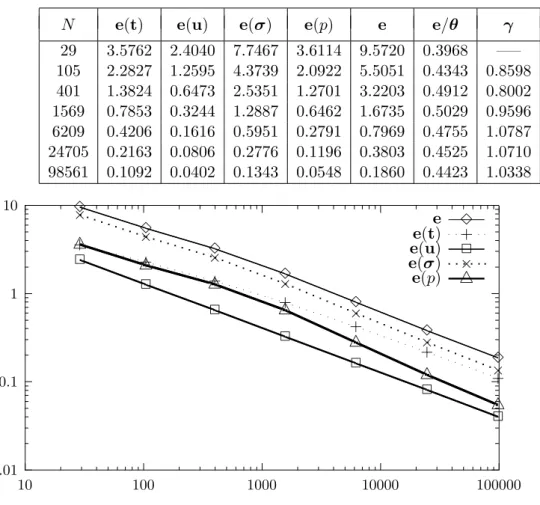
In Tables 5.1 and 5.2 we give the individual and global errors, the effectivity indexe/θ, and the experimental rate of convergenceγfor the uniform refinement as applied to Example 1 with pairs of parameters (α, ν) = (10,1) and (α, ν) = (100,1). In addition, Figures 5.1.1 and 5.2.1 show the corresponding individual errors versus the degrees of freedomN. We observe here that the rates of convergence behave as predicted by the theory, that is, of O(h), and that, due to the order of the constant ¯C(α, ν) in Theorem 3.2, some of these rates begin to deteriorate as α
increases. We also notice that the dominant components of the global error are given by e(t) ande(σ). Further, the effectivity indexes remain bounded above and below asN increases (with smaller lower bounds for bigger α), which confirms the reliability of θ and provides numerical evidences for it being efficient. However, as shown by Figures 5.1.2 and 5.2.2, and due to the fact that the solution of Example 1 is smooth, there is no relevant difference between the uniform and adaptive procedures for the global errore versusN.
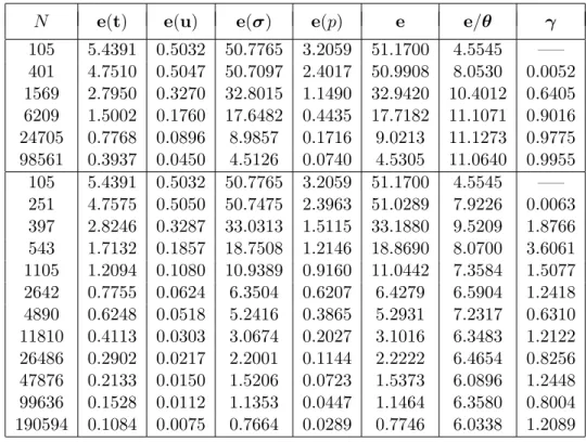
The numerical results concerning Example 2 are presented in Tables 5.3 and 5.4 where we display the individual and global errors, the effectivity index e/θ, and the experimental rate of convergence γ for both refinements with (α, ν) = (100,0.5) and (α, ν) = (1000,0.5). We note from these tables that only e(σ) constitutes now the dominant part of e. In addition, we observe a very clear difference between the uniform and adaptive refinements. The global error e of the latter decreases much faster than that of the former, thus recovering the rate of convergence O(h). As shown in Figures 5.3 and 5.4, this fact is even more pronounced for
α = 1000 where the convergence of the uniform refinement is very slow. However, although the effectivity indexes remain bounded above and below as N increases, for the two pairs of parameters and for both refinements, they also increase as α gets larger. Next, Meshes 5.3 and 5.4 display some intermediate meshes obtained with the adaptive refinement algorithm. It is interesting to confirm, as expected, that the procedure is able to recognize the boundary layer around (0,0). Also, we remark that this refinement is even more localized near the origin for
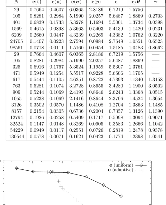
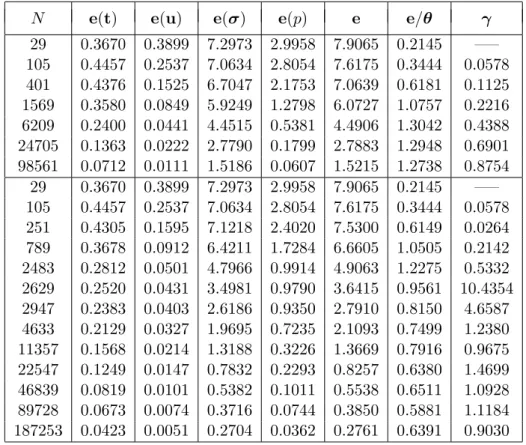
Next, Tables 5.5 and 5.6 provide the numerical results obtained for Example 3 with (α, ν) = (10,1) and (α, ν) = (100,1). As for the previous examples, e(σ) is again the dominant part of the global error e. Also, we observe that the effectivity indexes remain bounded above and below as the number of degrees of freedomN increases, with bounds close to 1.0, which confirms the reliability of θ and constitutes numerical evidences of its eventual efficiency. In addition, according to the experimental rates of convergence, which are also illustrated by Figures 5.5 and 5.6, the adaptive procedure yields again the quasi-optimal rate of convergence O(h) for the global errore. Moreover, as expected, the adaptive refinement algorithm is able to identify the singularities of the problem. In fact, as shown by Meshes 5.5 and 5.6, the adapted meshes are highly refined around the boundary point (1,1), in whose outer neighborhood the singularity lives. Further, similarly as for Example 2, the refinement is even more localized asαgets larger. Finally, the numerical results concerning Example 4 with (α, ν) = (1000,0.5) are collected in Table 5.7. The remarks and conclusions here are similar to those for Examples 2 and 3. Again, the effectivity indexes remain bounded, with bounds around 0.11, and, although the experimental rates of convergence of both refinements aproach 1 as N incresases, the global error of the adaptive one begins to decrease before than the uniform one. This fact is clearly observed in Figure 5.7 where the curve e versus N is shown. In addition, as expected, the corresponding adaptive refinement algorithm is able to recognize the inner layer of the problem. Indeed, as can be seen in Meshes 5.7, the adapted meshes are highly refined around the line
x2= 0.5−x1. We also notice here that the refinements identify a thin band exactly on this line, which corresponds to the flat behaviour of the solution caused by the power 2 in the exponent of the exponential function.
On the other hand, although we mentioned before that the solutions of the local problems (4.1) could be approximated via higher order H(div;T) subspaces, we show next that this additional computational effort would not necessarily improve the efficiency of the a-posteriori error estimate. To this end, we now identify the main components ofθ, which are given by those terms providing, respectively, the a-priori bounds for the local solutions ˆσT, and the residuals of the constitutive, equilibrium, and compressibility equations. More precisely, according to (4.6)
and (4.7), we can write θ = θ2ϕ + θ2res 1/2, where
θ2ϕ := X T∈Th
(
kth − ∇ϕhk2[L2(T)]2×2 +kuh−ϕhk2[L2(T)]2+h2T |ξh|2
)
+ X
e∈Eh(Γ)
kϕh− gk2
[H001/2(e)]2
,
and
θ2res := X T∈Th
(
kσh−νth+phIk2[L2(T)]2×2 + kf +div(σh)−αuhk2[L2(T)]2 + ktr (th)k2L2(T)
)
.
As general remarks, we would like to observe first that the numerical examples presented here behave much better than what the previous theoretical results insinuated. In particular, the order of the constants obtained in Theorems 3.1 and 3.2 indicate that the rates of convergence are affected by large values ofα, which, nevertheless, was not too severe in the examples. Further, since α is proportional to the inverse of the time-step ∆t, the estimates provided in these theorems also indicate that the convergence of time-dependent solutions should deteriorate as ∆tdecreases. Whether this holds exactly as predicted by the theory or behaves better than that is something to be seen from corresponding numerical results. Now, according to the constants in Theorem 4.1 and Lemma 4.3, one would have expected effectivity indexes between O(α−1) and O( αν3). However, as we could see, they all lie on ranges much tighter than that, they do not deteriorate as N increases, and they additionally improve when passing from uniform to adaptive refinements. The above observations yield the conjecture that these constants are overestimated and that they could be improved. In addition, our conclusion is that the proposed mixed method is perhaps not so competitive for extremely large values ofα, but it does constitute a good alternative for moderately large values of this parameter. Finally, we emphasize that the examples provide enough support for the adaptive algorithm being much more efficient than a uniform refinement when solving the discrete scheme.
References
[1] D.N. Arnold, J. Douglas Jr. and C.P. Gupta,A family of higher order mixed finite element methods for plane elasticity. Numerische Mathematik, 45, (1984), 1-22.
[2] N.S. Bakhvalov, Solution of the Stokes nonstationary problems by the fictitious domain method. Russian Journal of Numerical Analysis and Mathematical Modelling, 10, (1995), 163-172.
[3] R.E. Bank and A. Weiser,Some a posteriori error estimators for elliptic partial differ-ential equations. Mathematics of Computation,44, (1985), 283-301.
[4] G.R. Barrenechea and F. Valentin, An unusual stabilized finite element method for a generalized Stokes problem. Numerische Mathematik, 92, 4, (2002), 653-677.
[5] F. Brezzi, M. Fortin,Mixed and Hybrid Finite Element Methods. Springer Verlag, 1991.
[6] U. Brink and E. Stein,A posteriori error estimation in large-strain elasticity using equili-brated local Neumann problems. Computer Methods in Applied Mechanics and Engineering,
161, (1998), 77-101.
[7] J. Cahouet and J.P. Chabard, Some fast 3D finite element solvers for the generalized Stokes problem. International Journal for Numerical Methods in Fluids,8, (1988), 869-895.
[8] C. Calgaro and J. Laminie, On the domain decomposition method for the generalized Stokes problem with continuous pressure. Numerical Methods for Partial Differential Equa-tions, 16, 1, (2000), 84-106.
Table 5.1: individual errors, total errore, effectivity index, and global rate of convergence for the uniform refinement (Example 1, α= 10, ν = 1).
N e(t) e(u) e(σ) e(p) e e/θ γ
29 3.5762 2.4040 7.7467 3.6114 9.5720 0.3968 —– 105 2.2827 1.2595 4.3739 2.0922 5.5051 0.4343 0.8598 401 1.3824 0.6473 2.5351 1.2701 3.2203 0.4912 0.8002 1569 0.7853 0.3244 1.2887 0.6462 1.6735 0.5029 0.9596 6209 0.4206 0.1616 0.5951 0.2791 0.7969 0.4755 1.0787 24705 0.2163 0.0806 0.2776 0.1196 0.3803 0.4525 1.0710 98561 0.1092 0.0402 0.1343 0.0548 0.1860 0.4423 1.0338
0.01 0.1 1 10
10 100 1000 10000 100000
e 3 3 3 3 3 3 3 3
e(t) + + + + + + + +
e(u)
2 2 2 2 2 2 2 2
e(σ)
× × × × × × × ×
e(p)
4 4 4 4 4 4 4 4
Figure 5.1.1: errors vs. N for the uniform refinement (Example 1, α= 10, ν = 1).
0.1 1 10
10 100 1000 10000 100000 1e+06
e(uniform) 3 3 3 3 3 3 3 3 e(adaptive) + + + + + + + + + + + +
Table 5.2: individual errors, total errore, effectivity index, and global rate of convergence for the uniform refinement (Example 1, α= 100, ν = 1).
N e(t) e(u) e(σ) e(p) e e/θ γ
29 3.3494 2.3697 10.3296 4.1105 11.8504 0.0500 —– 105 2.0578 1.2424 7.7385 3.1434 8.6916 0.0700 0.4818 401 1.1765 0.6395 5.8418 2.3861 6.4509 0.1011 0.4449 1569 0.6821 0.3224 3.3689 1.4000 3.7254 0.1158 0.8048 6209 0.3909 0.1613 1.4540 0.6076 1.6317 0.1013 1.2003 24705 0.2109 0.0806 0.5048 0.2096 0.5914 0.0734 1.4697 98561 0.1084 0.0402 0.1765 0.0720 0.2230 0.0553 1.4095
0.01 0.1 1 10 100
10 100 1000 10000 100000
e 3 3 3 3 3 3 3 3
e(t)
+ + + + + + + +
e(u)
2 2 2 2 2 2 2 2
e(σ)
× × × × × × × ×
e(p)
4 4 4 4 4 4 4 4
Figure 5.2.1: errors vs. N for the uniform refinement (Example 1, α= 100, ν= 1).
0.1 1 10 100
10 100 1000 10000 100000 1e+06
e(uniform) 3 3 3 3 3 3 3 3 e(adaptive) + + + + + + + + + + + +
Table 5.3: individual errors, total errore, effectivity index, and global rate of convergence for both refinements (Example 2, α= 100, ν = 0.5).
N e(t) e(u) e(σ) e(p) e e/θ γ
105 5.4391 0.5032 50.7765 3.2059 51.1700 4.5545 —– 401 4.7510 0.5047 50.7097 2.4017 50.9908 8.0530 0.0052 1569 2.7950 0.3270 32.8015 1.1490 32.9420 10.4012 0.6405 6209 1.5002 0.1760 17.6482 0.4435 17.7182 11.1071 0.9016 24705 0.7768 0.0896 8.9857 0.1716 9.0213 11.1273 0.9775 98561 0.3937 0.0450 4.5126 0.0740 4.5305 11.0640 0.9955 105 5.4391 0.5032 50.7765 3.2059 51.1700 4.5545 —– 251 4.7575 0.5050 50.7475 2.3963 51.0289 7.9226 0.0063 397 2.8246 0.3287 33.0313 1.5115 33.1880 9.5209 1.8766 543 1.7132 0.1857 18.7508 1.2146 18.8690 8.0700 3.6061 1105 1.2094 0.1080 10.9389 0.9160 11.0442 7.3584 1.5077 2642 0.7755 0.0624 6.3504 0.6207 6.4279 6.5904 1.2418 4890 0.6248 0.0518 5.2416 0.3865 5.2931 7.2317 0.6310 11810 0.4113 0.0303 3.0674 0.2027 3.1016 6.3483 1.2122 26486 0.2902 0.0217 2.2001 0.1144 2.2222 6.4654 0.8256 47876 0.2133 0.0150 1.5206 0.0723 1.5373 6.0896 1.2448 99636 0.1528 0.0112 1.1353 0.0447 1.1464 6.3580 0.8004 190594 0.1084 0.0075 0.7664 0.0289 0.7746 6.0338 1.2089
0.1 1 10 100
100 1000 10000 100000 1e+06
e(uniform)
3 3
3
3
3
3
3
e(adaptive)
+ +
+ +
+
+ +
+ +
+ +
+
+
Table 5.4: individual errors, total errore, effectivity index, and global rate of convergence for both refinements (Example 2,α = 1000, ν= 0.5).
N e(t) e(u) e(σ) e(p) e e/θ γ
105 7.0383 0.0643 65.0020 5.0629 65.5777 1.0652 —– 401 12.9106 0.3337 334.0185 7.4337 334.3507 7.3412 —– 1569 17.7197 0.5382 538.4277 8.1264 538.7808 18.2978 —– 6209 12.7694 0.4502 450.3525 5.3283 450.5652 28.8851 0.2599 24705 7.1160 0.2680 268.0732 2.3559 268.1781 34.7400 0.7514 98561 3.7577 0.1404 140.4863 0.9185 140.5396 36.0464 0.9339 105 7.0383 0.0643 65.0020 5.0629 65.5777 1.0652 —– 251 12.9142 0.3338 334.0546 6.6592 334.3706 7.3370 —– 397 17.7427 0.5382 538.4458 7.0993 538.7851 18.2613 —– 543 12.8121 0.4501 450.2576 4.9853 450.4676 28.6842 1.1433 689 7.2888 0.2693 269.4196 2.6824 269.5316 33.3358 4.3135 835 4.7125 0.1543 154.4175 1.8963 154.5011 29.2990 5.7909 1722 2.7302 0.0798 79.8489 1.4523 79.9088 25.8793 1.8217 3839 1.6684 0.0463 46.3600 1.3075 46.4084 24.4862 1.3555 7031 1.2912 0.0363 36.4156 1.1266 36.4560 25.8745 0.7977 14781 0.8664 0.0239 24.0379 1.0019 24.0744 24.4694 1.1169 27310 0.6568 0.0182 18.2701 0.7172 18.2960 25.0696 0.8941 56312 0.4520 0.0123 12.3484 0.5608 12.3694 24.2670 1.0818 110822 0.3375 0.0090 9.0979 0.2983 9.1090 24.2919 0.9038
1 10 100 1000
100 1000 10000 100000 1e+06
e(uniform)
3
3 3 3 3
3
3
e(adaptive)
+
+ + + +
+
+ +
+ +
+ +
+
+
Meshes 5.3: adapted intermediate meshes with 26486 and 99636 degrees of freedom, respectively, for Example 2,α= 100, ν = 0.5.
Meshes 5.4: adapted intermediate meshes with 14781 and 56312
Table 5.5: individual errors, total errore, effectivity index, and global rate of convergence for both refinements (Example 3,α= 10, ν= 1).
N e(t) e(u) e(σ) e(p) e e/θ γ
29 0.7664 0.4607 6.0365 2.8186 6.7219 1.5756 —– 105 0.8281 0.2984 5.1990 2.0257 5.6487 1.8869 0.2703 401 0.6839 0.1733 5.3278 1.1694 5.5001 1.3734 0.0398 1569 0.4615 0.0898 5.3663 0.5403 5.4139 1.1420 0.0231 6209 0.2660 0.0447 4.3239 0.2269 4.3382 1.0762 0.3220 24705 0.1407 0.0223 2.7594 0.0984 2.7649 1.0551 0.6523 98561 0.0718 0.0111 1.5160 0.0454 1.5185 1.0483 0.8662 29 0.7664 0.4607 6.0365 2.8186 6.7219 1.5756 —– 105 0.8281 0.2984 5.1990 2.0257 5.6487 1.8869 —– 325 0.6916 0.1767 5.3524 1.1959 5.5307 1.3761 —– 471 0.5949 0.1254 5.5517 0.9228 5.6606 1.1705 —– 617 0.5444 0.1105 4.6251 0.8722 4.7393 1.1340 1.3158 763 0.5281 0.1074 3.2728 0.8655 3.4280 1.1900 3.0502 909 0.5244 0.1069 2.4193 0.8646 2.6243 1.3368 3.0515 1055 0.5238 0.1069 2.1416 0.8644 2.3706 1.4524 1.3654 3126 0.3502 0.0570 1.1486 0.4108 1.2704 1.3863 1.1485 8157 0.2154 0.0305 0.6736 0.2004 0.7357 1.3126 1.1390 12794 0.1926 0.0258 0.5409 0.1717 0.5998 1.3094 0.9071 32524 0.1147 0.0148 0.3269 0.0905 0.3583 1.2666 1.1042 54229 0.0949 0.0117 0.2551 0.0726 0.2819 1.2478 0.9378 130544 0.0578 0.0071 0.1621 0.0423 0.1774 1.2398 1.0541
0.1 1 10
10 100 1000 10000 100000 1e+06
e(uniform)
3 3
3 3
3
3
3
3
e(adaptive)
+
+ + +
+ +
++
+
+ +
+ +
+
+
Table 5.6: individual errors, total errore, effectivity index, and global rate of convergence for both refinements (Example 3,α= 100, ν= 1).
N e(t) e(u) e(σ) e(p) e e/θ γ
29 0.3670 0.3899 7.2973 2.9958 7.9065 0.2145 —– 105 0.4457 0.2537 7.0634 2.8054 7.6175 0.3444 0.0578 401 0.4376 0.1525 6.7047 2.1753 7.0639 0.6181 0.1125 1569 0.3580 0.0849 5.9249 1.2798 6.0727 1.0757 0.2216 6209 0.2400 0.0441 4.4515 0.5381 4.4906 1.3042 0.4388 24705 0.1363 0.0222 2.7790 0.1799 2.7883 1.2948 0.6901 98561 0.0712 0.0111 1.5186 0.0607 1.5215 1.2738 0.8754 29 0.3670 0.3899 7.2973 2.9958 7.9065 0.2145 —– 105 0.4457 0.2537 7.0634 2.8054 7.6175 0.3444 0.0578 251 0.4305 0.1595 7.1218 2.4020 7.5300 0.6149 0.0264 789 0.3678 0.0912 6.4211 1.7284 6.6605 1.0505 0.2142 2483 0.2812 0.0501 4.7966 0.9914 4.9063 1.2275 0.5332 2629 0.2520 0.0431 3.4981 0.9790 3.6415 0.9561 10.4354 2947 0.2383 0.0403 2.6186 0.9350 2.7910 0.8150 4.6587 4633 0.2129 0.0327 1.9695 0.7235 2.1093 0.7499 1.2380 11357 0.1568 0.0214 1.3188 0.3226 1.3669 0.7916 0.9675 22547 0.1249 0.0147 0.7832 0.2293 0.8257 0.6380 1.4699 46839 0.0819 0.0101 0.5382 0.1011 0.5538 0.6511 1.0928 89728 0.0673 0.0074 0.3716 0.0744 0.3850 0.5881 1.1184 187253 0.0423 0.0051 0.2704 0.0362 0.2761 0.6391 0.9030
0.1 1 10
10 100 1000 10000 100000 1e+06
e(uniform)
3 3 3
3
3
3
3
3
e(adaptive)
+ + + +
+ + +
+
+
+
+ +
+ +
Meshes 5.5: adapted intermediate meshes with 3126 and 54229 degrees of freedom, respectively, for Example 3,α = 10, ν = 1.
Meshes 5.6: adapted intermediate meshes with 4633 and 46839
Table 5.7: individual errors, total errore, effectivity index, and global rate of convergence for both refinements (Example 4,α = 1000, ν= 0.5).
N e(t) e(u) e(σ) e(p) e e/θ γ
105 74.3233 10.9499 975.4179 26.3889 978.6626 0.0838 —– 401 43.9757 7.2191 790.4335 25.1620 792.0885 0.1017 0.3156 1569 32.5849 4.0695 513.2866 11.7287 514.4697 0.1160 0.6326 6209 17.3618 2.1141 264.9580 5.2669 265.5869 0.1147 0.9613 24705 8.9221 1.0675 132.0790 2.1941 132.4025 0.1130 1.0080 98561 4.5016 0.5350 65.7869 0.8889 65.9489 0.1123 1.0074 105 74.3233 10.9499 975.4179 26.3889 978.6626 0.0838 —– 251 47.5896 7.5069 785.4328 25.8358 787.3331 0.0978 0.4992 907 34.5913 4.2248 536.2225 13.2819 537.5178 0.1164 0.5942 2111 20.9361 2.1538 292.7591 8.1437 293.6276 0.1247 1.4315 7141 11.2381 1.1037 148.3617 4.1104 148.8476 0.1240 1.1149 17599 9.4008 0.6518 91.1181 3.1416 91.6579 0.1334 1.0750 30105 5.9042 0.5120 68.4031 2.1752 68.6938 0.1244 1.0744 87607 4.1128 0.2886 41.6759 1.6638 41.9124 0.1367 0.9250 120853 3.5184 0.2520 33.8690 1.3457 34.0788 0.1243 1.2862
10 100 1000
100 1000 10000 100000 1e+06
e(uniform) 3
3
3
3
3
3
3
e(adaptive)
+ +
+
+
+
+ +
+ +
+
Table 5.8: Main components of the a-posteriori error estimate θ.
Example 1 (α= 10, ν = 1) Example 1 (α= 100, ν = 1)
N θϕ θres
29 4.5135 23.6942 105 2.5688 12.4118 401 1.5104 6.3792 1569 0.8615 3.2136 6209 0.4659 1.6099 24705 0.2404 0.8053 98561 0.1213 0.4027
N θϕ θres
29 4.3964 236.8632 105 2.4076 124.1070 401 1.3361 63.7909 1569 0.7612 32.1361 6209 0.4345 16.0988 24705 0.2346 8.0533 98561 0.1205 4.0271
Example 2 (α= 1000, ν = 0.5) Example 3 (α= 10, ν = 1)
N θϕ θres
105 61.5259 2.1109 251 45.5072 2.4457 397 29.3608 2.9050 543 15.4992 2.5303 689 7.8532 1.9235 835 4.9966 1.6857 1722 2.8452 1.1997 3839 1.7123 0.8124 7031 1.3031 0.5357 14781 0.8945 0.4096 27310 0.6765 0.2737 56312 0.4681 0.2018 110822 0.3512 0.1313
N θϕ θres
29 1.9781 3.7799 105 1.3309 2.6815 325 0.8823 3.9209 471 0.6377 4.7937 617 0.5360 4.1447 763 0.5107 2.8349 909 0.5060 1.8968 1055 0.5053 1.5520 3126 0.3455 0.8487 8157 0.2140 0.5180 12794 0.1890 0.4173 32524 0.1141 0.2589 54229 0.0942 0.2054 130544 0.0576 0.1310
Example 3 (α= 100, ν = 1) Example 4 (α= 1000, ν = 0.5)
N θϕ θres
29 1.7393 36.8189 105 1.1333 22.0862 251 0.7085 12.2245 789 0.4471 6.3244 2483 0.2940 3.9861 2629 0.2491 3.8005 2947 0.2356 3.4162 4633 0.2104 2.8048 11357 0.1580 1.7195 22547 0.1249 1.2881 46839 0.0824 0.8465 89728 0.0680 0.6510 187253 0.0427 0.4300
N θϕ θres
[10] G.N. Gatica,An application of Babuˇska-Brezzi’s theory to a class of variational problems. Applicable Analysis,75, 3-4, (2000), 297-303.
[11] G.N. Gatica, Solvability and Galerkin approximations of a class of nonlinear operator equations. Zeitschrift f¨ur Analysis und ihre Anwendungen, 21, 3, (2002), 761-781.
[12] G.N. Gatica, M. Gonz´alez and S. Meddahi,A low-order mixed finite element method for a class of quasi-Newtonian Stokes flows. PartI: a-priori error analysis. Computer Me-thods in Applied Mechanics and Engineering, vol. 193, 9-11, pp. 881-892, (2004).
[13] G.N. Gatica, M. Gonz´alez and S. Meddahi,A low-order mixed finite element method for a class of quasi-Newtonian Stokes flows. PartII:a-posteriori error analysis. Computer Methods in Applied Mechanics and Engineering, vol. 193, 9-11, pp. 893-911, (2004).
[14] G.N. Gatica, N. Heuer and S. Meddahi,On the numerical analysis of nonlinear two-fold saddle point problems. IMA Journal of Numerical Analysis, 23, 2, (2003), 301-330.
[15] G.N. Gatica and E.P. Stephan,A mixed-FEM formulation for nonlinear incompressible elasticity in the plane. Numerical Methods for Partial Differential Equations, 18, 1, (2002), 105-128.
[16] G.M. Kobelkov and M.A. Olshanskii,Effective preconditioning of Uzawa type schemes for a generalized Stokes problem. Numerische Mathematik, 86, (2000), 443-470.
[17] O. Ladyzhenskaya,New equations for the description of the viscous incompressible fluids and solvability in the large for the boundary value problems of them. In Boundary Value Problems of Mathematical Physics V, AMS (Providence), 1970.
[18] J.L. Lions and E. Magenes,Probl`emes aux Limites non Homog`enes et Applications. I. Dunod, Paris, 1968.
[19] B.V. Pal’tsev,On rapidly converging iterative methods with incomplete splitting of bound-ary conditions for a multidimensional singularly perturbed system of Stokes type. Russian Academy of Sciences, Sbornik Mathematics,81, (1995), 487-531.
[20] J.E. Roberts and J.-M. Thomas,Mixed and Hybrid Methods. In Handbook of Numerical Analysis, vol. II, edited by P.G. Ciarlet y J.L. Lions, North-Holland (Amsterdam), 1991.
[21] V. Sarin and A. Sameh,An efficient iterative method for the generalized Stokes problem. SIAM Journal on Scientific Computing,19, 1, (1998), 206-226.
[22] B. Scheurer, Existence et approximation de point selles pou certain problemes non-lin´eaires. RAIRO Analyse Num´erique, 11, 4, (1977), 369-400.