Degrees of freedom and model selection in semiparametric additive monotone regression

Degrees of freedom and model selection in

semiparametric additive monotone regression.

Cristina Rueda1

University of Valladolid. Spain

Abstract

R The degrees of freedom of semiparametric additive monotone models are derived using results about projections onto sums of order cones. Two impor-tant related questions are also studied, namely, the definition of estimators for the parameter of the error term and the formulation of specific Akaike In-formation Criteria statistics. Several alternatives are proposed to solve both problems and simulation experiments are conducted to compare the behav-ior of the different candidates. A new selection criterion is proposed that combines the ability to guess the model but also the efficiency to estimate the variance parameter. Finally, the criterion is used to select the model in a regression problem from a well known data set.

Keywords: additive models, isotonic models, order restricted inference, Akaike information criterion.

1. Introduction

Semiparametric monotone additive models are receiving special attention in the statistical literature because they are pragmatic alternatives to linear and nonparametric models. There are several main advantages. First, the flexibility, including more forms of regression than the rigid linear formula-tion. Second, the simple additive structure that guarantees, as shown below, the solution of the estimation problem with a relatively simple algorithm. Third, the incorporation of the monotonicity restriction avoids the problem

Email address: [email protected](Cristina Rueda )

1_{Address: Prado de la Magdalena s/n. Facultad de Ciencias. Dpto. Estadistica.}

of defining user-specified choices, such as bandwidth, or smoothing parame-ters or number and placement of knots, typical drawbacks of nonparametric methods as kernel smoother, smoothing splines and regression splines, being in this sense a robust methodology. And finally, the oracle property, which implies that the rate of convergence of the least-square estimate of each ad-ditive component is independent of the number of adad-ditive components in the model (see Chen (2009) and references therein).

The usefulness of monotone models is wide, the papers by Morton-Jones et al. (2000), Hussian et al. (2004), and De Boer et al. (2002) give some applications in the biomedical, environmental and toxicology fields respec-tively. These are only a few among many others in different fields. There are a lot of settings where isotonic models are suitable as monotone relationships frequently appear in real practice. Two illustrative examples are: first, the relation between the risk of getting a disease and exposure, in epidemiolog-ical applications, where the risk is often known to decrease with increasing exposure; and second, the prediction of sociological indexes that are known to monotonically change with important predictors, as is the case in the ex-ample analyzed in section 4. Besides, the incorporation of linear terms is useful to model dummy explanatory variables and also to decrease the risk of overfitting.

The semiparametric additive monotone regression model is defined by:

yi =α+ p

X

j=1

βjxji+ q

X

j=1

hj(zji) +εi, i= 1, ..., n, (1)

where y = (y1, ..., yn)0 is the response vector, xj = (xj1, ..., xjn)0, j =

1, ..., pandzj = (zj1, ..., zjn)0, j = 1, ...q,are linearly independent explanatory

variables, andε= (ε1, ..., εn)0is a random error term. It is assumed that each

hj() is a monotone function, which is suppose to be monotone increasing

with-out loss of generality, and thatε∼N(0, W−1_σ2_{), whereW =diag(w}

1, ..., wn)

is a matrix of known weights (by instances, in experiments with replicaswi is

the number of replicas under each condition) and σ is unknown. The MLEs (α,_b βb₁, ...,βb_p,bh₁, ...,bh_q) are the solution of the optimization problem:

min

n

X

i=1

wi(yi−α− p

X

j=1

βjxji− q

X

j=1

hj(zji))2

!

subject to the restriction thatα ∈ <, β ∈ <p _{and each h}

j() is monotone

and verifies the standard identifiability condition

n

P

i=1

hj(zji) = 0.

In fact, the solution to the optimization problem (2) is not unique, any other set of monotone functionsmj, j = 1, ..., q, verifyingmj(zji) =bh_j(z_ji), j =

1, ..., q;i= 1, ..., nwould have also solved the least square minimization. De-fineθ0 =α−

p

P

j=1

βjxji;θj =hj(zj), j = 1, ..., qadnθ =θ0+θ1+...+θq. Then,

the least-square estimator_by= (_by1, ...,byn)

0_{, where} b

yi =αb+βb1x1i+...+βbpxpi+ b

h1(z1i)+...+bh_q(z_qi) =θb₀+θb₁+...+θb_q, is theL₂-projection with weightsW of

the observed vectoryontoK,pw(y/K), whereK =L0+S1+...+Sq is a

con-vex cone in <n _{defined by the restrictions imposed, L}

0 being the linear sub-space of dimensionp+1 spanned by columns in matrix (1n, x1, ..., xp) and each

Sj being the order cone associated to zj, Sj = {u ∈ <n

u1j ≤...≤unj},

where (1j, ..., nj) is a permutation of (1, ..., n) verifying zj1j ≤ ... ≤ zjnj (if

several observations have the same value of the predictor zj, define Sj using

equalities instead of inequalities between the coordinates corresponding to these observations). A simple example that illustrates how the cone K is derived from the initial information on the explanatory variables is given in section 2. Therefore, the model that dealt with in this paper can be expressed in a simplified form as:

y=θ+ε, θ ∈K;ε∼N(0, W−1σ2).

Without loss of generality, it can be assumed thatW =Isince a linear change of variable can be made to the unweighted case by considering y∗ = W1/2_y and the cone K∗ = W1/2K. Then, pw(y/K) = W−1/2p(y∗/K∗), which

im-plies that most properties of the projections in the weighted case are derived from those in the unweighted case, in particular those proved or used in this paper. In addition, the calculation of pw(y/K) can be accomplished via the

PAVA (Pool Adjacent Violators Algorithm) when K is an order cone as Sj,

and the algorithm to obtain the projection when K is the sum of several of these cones is a general PAVA, which also works with weights. (see Meyer (1999) and Robertson et al (1988) for the properties of the weighted pro-jections and the computational algorithms). Therefore, in the following the notation for the weighting is dropped to simplify the presentation and the solution to the optimization problem can be expressed as,

b

θK = arg min

θ∈Kky−θk

2

where kuk2 =

n

P

i=1

u2

i.

The simple additive structure of the model guarantees the solution of the optimization problem with a relatively simple algorithm and good properties of estimators. Mammen and Yu (2007) derive a backfitting algorithm, a cyclic PAVA, to get the estimators, and show the oracle property for the model without linear terms; and Cheng (2009) extends the results to the general case and derives the asymptotic distribution of the regression estimators.

Before the publication of the papers mentioned in the last paragraph, other authors dealt with this type of models. Some important references are Stone (1982) and Stone (1985), who studied the rates of convergence of re-gression estimators and first showed the oracle property for additive models; Bachetti (1989) who first estimated the additive functions with backfitting; and Huang (2002) who dealt with the case q = 1. There have also been many other authors, who have dealt with additive models or isotonic regres-sion models, whose research has been the basis for recent development. We highlight the works by Brunk (1970), Hanson (1973), Dykstra (1983), Hastie and Tibsirani (1986), among many others.

However, there is still an unsolved and important question around these models that has to do with the determination of the degrees of freedom or the dimensionality of the model. Several authors have dealt with the question of dimensionality. Meyer and Woodroofe (2000) dealt with the univariate monotone and shape regression models, while Kato (2009) dealt with the question in shrinkage regression with application to the Lasso. For a general convex cone C, these authors introduced the concept of degrees of freedom of the associated model, also called the divergence, which is defined by DC(y)

as follows:

DC(y) = divC(θb_C) =

n

X

i=1

∂ ∂yi

b

θi(y), (4)

where, θbC(y) =p(y/C) = (θb1(y), ...,θbn(y))0.

When q = 0 (p = 0 and q = 1), the cone K is defined using inequality restrictions andDK(y) is easily derived asdim(LyK), whereL

y

Kis the subspace

defined by the inequalities that the projection verifies as equalities and verifies

In these cases, the convex cone is expressed explicitly by a set of linear inequalities and equalities.

However, the derivation of DK(y) is not straightforward in the general

case q > 0 and p > 0 from the results in previous papers. The aim of this paper is to achieve it in a simple way.

The derivation ofDK(y) is also relevant for solving two important aspects

in model fitting the estimation of σ and the model selection. In the former, the degrees of freedom is used to correct the bias of the MLE estimator and in the latter to derive the AIC measure penalty term. Several authors have considered the first problem in univariate regression, Meyer (2000) and Rueda et al. (2010) among others. But again, as far as we know, the question is not solved in the general case. On the other hand, the problem of variable selection is a very important problem in statistical modeling that has recently gained a lot of attention in semiparametric models (see Li and Liang (2008) and Xiao et al. (2010) among others). The AIC approach is considered in this paper for this question. In this paper, several alternative proposal are given to solve both questions which are validated with numerical simulations and in a example.

The outline for the rest of the paper is as follows: in section 2, a practical formula for DK(y) for semiparametric additive monotone models is derived

using new algebraic results in relation with the projection onto the sum of order cones. In section 3, the question of the estimation ofσis discussed and a new AIC criterion for model selection that uses a corrected bias estimator for

σ is proposed. The estimator and the criterion are validated using simulation experiments. Finally, the results are applied in section 4 to the well known Prestige data set and some general conclusions are given in section 5.

2. Degrees of freedom

In this section, the subscript K is eliminated from θband D(y) to make

the presentation easier. The solution to the optimization problem (3) is then given by bθ=p(y/K), which is the maximum likelihood estimator ofθ.

Ly_K =nu∈ </a0_iu= 0, for all i for which a0_iθb(y) = 0 o

.

LetF_Ky =Ly_K∩K , the set of polyhedral conesF_{K y}y are called faces ofK

and eachLy_K is the linear subspace associated with the faceF_Ky . The faces of a polyhedral cone are involved in the algebraic result derived in this section. Lemma 2.1(i), below, shows that K =L0 +S1 +...+Sq is a polyhedral

cone (this is a known result given here for completeness). Lemma 2.1 (ii) and (iii) give other results on projections on convex cones that will be used later on.

However,D(y) cannot be derived from Lemma 2.1(i) in a straightforward manner because it does not provide an explicit version ofK as a set of linear inequality restrictions.

In the simple case ofL0 and eachSj being orthogonal linear subspaces, we

have, from the properties of projections, thatp(y/K) = p(y/L0) +p(y/S1) +

... +p(y/Sq) and also that D(y) = dim(L0) + dim(S1) + ... + dim(Sq).

Even in the case where orthogonality is not verified but each Sj is a linear

subspace, the dimension can be derived from the individual dimensions and dimensions on the intersections. In the case q = 1, the equation is very simple: D(y) = dim(L0 +S1) = dim(L0) + dim(S1)−dim(L0 ∩S1). This is not true when Sj are cones, as the example shows. The example also

illustrates the derivation of D(y) in a simple case.

Example Letn = 3, z = (3,2,1), x=

  1 1 1 1 1 0  .

L0 ={u∈ <3/u1 =u2}, S1 ={u∈ <3/u1 ≥u2 ≥u3}, L0∩S1 ={u∈ <3/u1 =u2 ≥u3}. dim(L0) + dim(S1)−dim(L0∩S1) = 2 + 3−2 = 3.

Lety= (y1, y2, y3) = (1,2,2), the backfitting algorithm (Cheng (2009))is applied to find θb(y). The runs of the algorithm are as follows:

b

θ(0)₀ (y) = (y, y, y);θb

(1)

0 (y) = (0,0,0)

b

θ(1)₀ (y) = p(y−θb

(0)

1 (y)/L0) = (

y1+y2

2 ,

y1+y2

2 , y3);

b

θ(1)₁ (y) = p(y−θb

(1)

0 (y)/S1) = (0,0,0).

Then,θb(y) =θb₀(y) +θb₁(y) = (y1+₂y2,y1+₂y2, y₃) + (0,0,0).

Now,D(y) = 3

P

i=1

∂

∂yibθi(y) =

3 P i=1 ∂ ∂yi 1 P j=0 b

θji(y) = 2.

solve the problem, as in the example above, any representation of θbwill be

used from the backfitting algorithm that is given by: θb=θb₀ +θb₁+...+θb_q, b

θ0 ∈L0,θb_j ∈S_j, j = 1, ..., q.

To make this representation useful to derive D(y), lemma 2.2 (i) proves that D(y) = dim(L0 +Ly1 +...+Lyq), where each L

y

j is the linear subspace

associated with a face of the cone Sj such as bθ_j ∈ Ly_j. Lemma 2.2(ii) also

provides an easy way to calculate D(y) in practical applications. The proofs of the two lemmas are deferred to the appendix.

Lemma 2.1. (i) Let L be a linear subspace and let Cj, j = 1, ..., q be

poly-hedral cones. Then K =L+C1+...+Cq is a polyhedral cone.

(ii) Let L and C be a linear subspace and a convex cone respectively and let L⊂C. Then, C =L+C∩L⊥ and p(y/C) = p(y/L) +p(y/L⊥∩C).

(iii) Let L and C be a linear subspace and a convex cone respectively. Then, p(y/L+C) = p(y/L) +p(y/L⊥∩(L+C)).

Lemma 2.2. LetK =L0+S1+...+Sq be a convex cone whereL0 is a linear

subspace and each Sj is an order cone. For a given y ∈ <n, the backfitting

algorithm gives: p(y/K) = θb=θb₀+bθ₁+...+θb_q, θb₀ ∈L₀, θb_j ∈S_j,j = 1, ..., q.

Then,

(i) D(y) = dim(L0 +L1y +...+Lyq), where each L y

j is a linear subspace

associated with a face of Sj that has θbj as an interior point.

(ii) Let us denote{aji} Nj

i=1 as theNj different components of θbj. For each

j = 1, ..., q and i= 1, ..., Nj, let vji be the n-dimensional vector defined by

vi_jk = 1 ⇐⇒θb_jk =a_ji, v_jki = 0⇐⇒θb_jk 6=a_ji, k = 1, ..., n.

Then, for each j, dim(Ly_j) = Nj, and the set

vi j

Nj

i=1 is a minimal set of

generators for Ly_j.

Remark From the generators for the subspaces, Ly_j j = 1, .., q, given in Lemma 2.2(ii), select a maximal set of linearly independent vectors and define a matrix, V, with these vectors as columns. Then, rank(V,1n, x1, ...xp) =

D(y).

Moreover, from the properties of projection onto the sum of subspaces, we have that,

D(y) = dim(L0+Ly1+...+L

y

q) = p+1+dim(L y

1+...+L

y

q)−dim(L0∩(Ly1+...+L

and,

dim(Ly₁+...+Ly_q) = X

j

dim(Ly_j)−X

l,j

dim(Ly_l∩Ly_j)+X

l,m,j

dim(Ly_l∩Ly_m∩Ly_j)−....

=X

j

Nj−

X

l,j

Nl,j+

X

l,m,j

Nlmj −...,

whereNj is the number of different values in the set

n

b

θji

on

i=1

, Nlj is the

number of different values that occur simultaneously (in the same coordi-nates) in the sets nθb_ji

on

i=1

and nθb_li on

i=1

, etc... We then have a constructive equation that shows the contribution of the linear component, the monotone components and the intersections to D(y).

3. Variance estimation and AIC statistics

3.1. Discussion and definitions

Let us consider first the estimation of σ2_{. The problem of the bias of}

b

σ2

M LE =

ky−θc_Kk 2

n is a well known problem in linear modeling, where K =L

is a linear subspace and an unbiased estimator is usually defined as σ_{bU B}2 =

ky−θcKk 2

n−DK(y), in which DK(y) = p+ 1 is the total number of coefficients in the

linear model.

Sampson et al. (2003) deal with the problem in monotone regression when

n = 2 and propose the use of _bσ2

U B. Also, Rueda et al. (2010) use the latter

estimator to estimate the variance in a univariate monotone mixed model. On the other hand, in monotone univariate regression problems, Meyer and Woodroofe (2000) propose an estimator for σ2 _{that corrects the bias, as} follows:

b

σ_{M W}2 =

y−θbK

2

n−M in(1.5DK(y), n/2)

.

The estimator above uses the penalty 1.5DK(y) instead of DK(y) in the

denominator. An insight behind this correction is given below in Lemma 3.1. Moreover, the final version of the penalty asM in(1.5DK(y), n/2) assure that

b

σ2

In this paper, two estimators are defined for the semiparametric model following the research of these authors. Lemma 3.1, below, shows an inequal-ity that will be useful to derive the estimators. The proof of the lemma is deferred to the appendix.

Lemma 3.1. Let y =θ+ε, θ∈C;ε∼Nn(0, σ2I) where, C =L+C0, L is

a linear subspace of dimension r and C0 a convex cone. Then, ∃c ∈ <,2 ≥

c≥1 such as:

E

y−θbC

2

σ2 =n−c(EDC(y)−r)−r.

From lemma 3.1, applied to K = L0 +S1 +...+Sq, we have the following

equation,

E

y−θbK

2

σ2 =n−c(EDK(y)−p−1)−(p+ 1), for a given unknown c, 2≥c≥1.

The quantity cdepends on θ but it is not strainforward to estimate. We consider two values that have also been considered before in the literature. Firstly, the smallest value, c= 1, is considered as it is the natural extension to the linear case and it has been successfully used by Rueda et al (2010), even though it provides a positive biased estimator. Secondly, in order to correct the positive bias, we consider c= 1.5 as a compromise intermediate value that has been also considered by Meyer and Woodroofe (2000). These authors have studied the behavior of other choices and their recommendation is to use c= 1.5 to correct the bias of the estimator with the inclusion of an upper limit. The corresponding estimators for σ2 _{are given by:}

b

σ_K,2 _1.5 =

y−θbK

2

n−M in(1.5DK(y)−0.5(p+ 1), n/2)

; σ_bK,2 ₁ =

y−θbK

2

n−DK(y)

.

The AIC approach is considered for the second question. The AIC is a very popular criterion to model selection in a broad class of statistical problems. From the definition of the first AIC statistics, Akaike (1973), there has been a very large number of papers dedicated to the definition of alternative AIC for specific applications. Isotonic models are no exception: Kato (2009) proposes to use a standard AIC statistic with penalty term equal to 2DK(y), while Zhao and Peng (2002) and Liu et al (2009) propose AIC

measures with smaller penalty terms. However, these measures have not been validated in regression scenarios. Different proposals to solve both questions are provided and validated in this paper.

Now, in order to define the AIC measures, let us consider for the moment that σ is a known parameter. Usually, the AIC is defined as a penalized loglikelihood. AIC(θb) = −2l(θb) + 2k, where k is the number of parameters

in the model and accounts for the bias when estimating the expected log-likelihood (l(θb). In the context of the model subject to restrictions on the

parameters given by a cone K, Anraku (1999) shows that the bias is the following quantity:

b(θ) = n

2 + 1 2σ2Eθ(

θ−θbK

2

− y−θbK

2 ). It is straight forward to show that:

b(θ) = _2σ12Eθ(ky−θk

2 +

θ−θbK

2

− y−θbK

2 ) = = 1

σ2Eθ(< y−θ,θb_K−θ >) =E_θ(D_K(y)),

where the last equality follows from Stein’s (1981) lemma.

Thus, we can define an AIC criterion for restricted regression when σ is known as follows:

AIC(θb_K) = −2l(θb_K) + 2E_θD_K(y).

In the framework of simple order restricted mean problems, several au-thors have dealt with the question, giving different proposals. Anraku(1999) proposes using ORICA(θb) = −2l(θb) + 2B, where B = infθEθ(DK(y)) =

Eθ0(DK(y)), where θ0 ∈ LK, the largest subspace verifying LK ⊂ K. Then,

B is usually too small, except when θ ∈LK, which is a very strong

assump-tion.

Also, Zhao and Peng (2002) and Liu et al. (2009) propose the use of a penalty term defined by 2λDK(y), where λ <1 and is chosen from different

They consider simulations with very small values of n (n≤ 5) and compare the performance of the new criterion only against the ORICA(θb_K) and the

standard AIC with a penalty term equal toDK(y). These results are not very

relevant for our problem, asnis much higher in regression contexts, there are no replications and the focus is on the model selection within a wider family of models. However, for comparative purposes, an AIC measure defined us-ing a penalty 2K(y) with λ <1 has also been considered, to show the effect

of reducing the penalty. From the several choices in the literature, which usually depends on n, (see Zhao and Peng (2002)), we have selected, for our simulations, the value λ = 0.75 . It is not worth to test other alternatives because numerical result clearly point out that λ = 1 is the best choice in this context.

Moreover, there is the problem of σ being unknown. It is hopeless to derive the corresponding AIC criterion in this case if the properties of the candidate estimators for σ cannot be obtained. A simple approach is there-fore followed and the following general criterion is proposed:

AICλ,µ(bθK) =−2l(θbK,bσK,µ) + 2λDK(y),

where λ ∈ {1,0.75} and µ∈ {1,1.5}. In preliminary studies, smaller values for λ have also been considered but, as their performance is bad, they are not include here in order to simplify the output.

For a given pair (λ, µ),letK∗ = arg_KminAICλ,µ(bθ_K) be the cone

associ-ated to the selected model andσ_b∗ =_bσK∗_,µthe corresponding estimator for σ. The MSE of _bσ∗ will be estimated in the simulations, besides the probability of correct detection, to determin the goodness of the AICλ,µ(θb_K) criterion.

On the other hand, when the MLE for σ is used instead of σ_bK,µ the AIC

statistic reduces to:

AICλ,M LE(θbK) = log(bσM LE) + 2λDK(y), λ∈ {1,0.75}.

AIC1,M LE(θb_K) is the most widely used AIC statistic in the literature when

σ is unknown. As shown below, the performance of AIC1,M LE(θb) is worse

than the new proposals in most scenarios.

Finally, for the case when σ is known, we consider:

AICλ(θb_K) = −2l(θb_K) + 2λD_K(y), λ∈ {1,0.75}.

3.1.1. Monte Carlo studies

Two simulation experiments, A and B, have been conducted. A uses sim-ulated independent explanatory variables and B uses the explanatory vari-ables from the example in section 4. In both cases, the sample size equals 102, which is the sample size in the example.

The data generating model in experiment A is an additive regression model of the form:

y= 3

P

j=1

mj(uj) +ε,

with predictor vector u1, u2, u3 i.i.d U[0,1] 102

, ε ∼ N102(0, σ2I) and σ ∈

{1,5}.The functions P

mj() have been defined, in four different forms,

fol-lowing the suggestions of other authors (Borra and Ciaccio(2002), Curtis and Ghosal(2010) and Yang(2008)) as follows:

M1 : exp(1.1u3₁) +log((e2−1)u2+ 1)−sin(2πu3);

M2 : exp(1.1u3₁)−sin(2πu2) +u3;

M3 : −sin(2πu1) +u2+ 5u3;

M4 : u1+ 2u2+ 3u3.

M1 is a nonparametric model in the three components (p = 0, q = 3), M2 is nonparametric in the first two components and linear in the third (p = 1, q= 2), M3 is nonparametric in the first component and linear in the rest (p= 2, q = 1) andM4 is a linear model (p= 3, q = 0). In each scenario, the same four models have been fitted with intercept.

On the other hand, the data generating model in experiment B, is given by:

y= 3

P

j=1

hj(xj) +ε,

the predictor vectorsx1, x2, x3being the explanatory variables in the Pres-tige data set (section 4), ε N102(0, σ2I) and σ∈ {2,10}.The selection of other values for σ to those in experiment 1 allows to show the performance of the approaches under different uncertainty levels. The functions hj() have

b

σ σ M1 M2 M3 M4 H1 H2 H3 H4

b

σ1.5, low 0.0086 0.0076 0.0066 0.0056 0.3527 0.1795 0.0306 0.0245

b

σ1 low 0.0108 0.0056 0.0060 0.0056 0.3249 0.2131 0.0435 0.0245

b

σM LE low 0.0330 0.0131 0.0069 0.0401 0.9850 0.7440 0.2013 0.0269

b

σ1.5 high 0.1535 0.1604 0.1459 0.1406 1.0487 0.9070 0.6305 0.6124

b

σ1 high 0.1951 0.1648 0.1483 0.1406 2.1531 1.6040 0.7622 0.6124

b

σM LE high 0.4897 0.3194 0.2158 0.1609 6.8484 4.6655 1.7758 0.6731

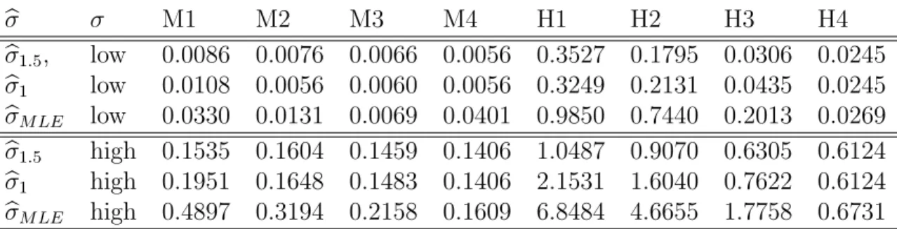
Table 1: MSE for _bσ1.5, _bσ1,and_bσM LE under different scenarios.

forms, as follows:

H1 : 15logx1+x42/2000−log(x3 + 1);

H2 : 15logx1+x42/2000;

H3 : 8(x1−x1)/sx1 +x

4 2/2000;

H4 : 8(x1−x1)/sx1 + (x2−x2)/sx2.

H1 is a monotone model in the three components, H2 is monotone in the first two components, H3 is linear in the first component and monotone in the second and H4 is a linear model in the first two components. In each scenario the same four models have been fitted.

A total of 16 scenarios, eight models with low and high values forσ, have been simulated, 100 replications were generated in each scenario and for each data set four models were fitted being among them the correct one. The simulation addresses two questions. First, which estimator of σ is preferred in terms of MSE?. Second, which of the AIC statistics defined in section 3.1 performs better?. For the first question, assuming the correct model, the empirical estimators of the MSE are derived for the new proposals. For the second question, the four models fitted are considered and for each of the 16 scenarios and each criterion, AICλ,µ, the frequency of correct detection

(FCD) is derived and the empirical estimator of the MSE ofσ_b∗ are obtained, where _bσ∗ has been defined in section 3.1. A good criterion should be one with a high FCD that gives an accurate estimator for σ under the selected model. The FCD of AICλ and AICλ,M LE and the MSE of σM LE have also

been obtained for comparative purposes.

AIC σ M1 M2 M3 M4 H1 H2 H3 H4 Mean

AIC1,1.5 low 0.78 0.41 0.53 0.61 0.99 0.53 0.15 0.70 0.59

AIC1,1 low 0.90 0.40 0.44 0.36 0.93 0.59 0.16 0.46 0.53

AIC1,M LE low 0.99 0.36 0.23 0.25 0.99 0.53 0.02 0.32 0.46

AIC.75,1.5 low 0.98 0.30 0.21 0.13 0.99 0.47 0.01 0.26 0.42

AIC.75,1 low 1.00 0.20 0.10 0.05 0.98 0.54 0.02 0.10 0.37

AIC.75,M LE low 1.00 0.17 0.04 0.01 0.99 0.47 0.01 0.04 0.34

AIC1 low 0.79 0.42 0.52 0.73 0.58 0.72 0.70 0.78 0.66

AIC.75 low 1.00 0.26 0.16 0.16 0.75 0.63 0.28 0.39 0.45

AIC1,1.5 high 0.13 0.09 0.15 0.59 0.32 0.59 0.25 0.58 0.34

AIC1,1 high 0.18 0.12 0.14 0.55 0.43 0.58 0.19 0.53 0.34

AIC1,M LE high 0.24 0.11 0.15 0.48 0.51 0.58 0.14 0.49 0.34

AIC.75,1.5 high 0.46 0.17 0.17 0.24 0.45 0.61 0.21 0.31 0.33

AIC.75,1 high 0.50 0.16 0.12 0.18 0.60 0.48 0.12 0.26 0.30

AIC.75,M LE high 0.58 0.10 0.10 0.16 0.74 0.42 0.11 0.16 0.30

AIC1 high 0.13 0.09 0.12 0.59 0.23 0.64 0.23 0.72 0.34

AIC.75 high 0.48 0.16 0.16 0.26 0.45 0.62 0.20 0.33 0.33 Table 2: FCD for different AIC statistics and simulated sccenarios.

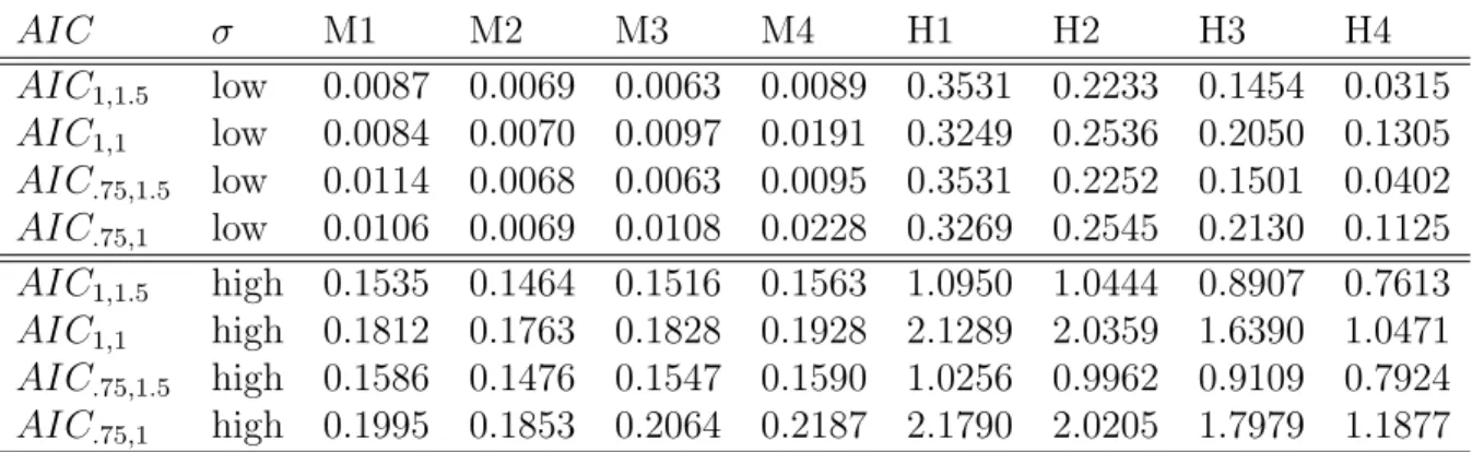
AIC σ M1 M2 M3 M4 H1 H2 H3 H4

AIC1,1.5 low 0.0087 0.0069 0.0063 0.0089 0.3531 0.2233 0.1454 0.0315

AIC1,1 low 0.0084 0.0070 0.0097 0.0191 0.3249 0.2536 0.2050 0.1305

AIC.75,1.5 low 0.0114 0.0068 0.0063 0.0095 0.3531 0.2252 0.1501 0.0402

AIC.75,1 low 0.0106 0.0069 0.0108 0.0228 0.3269 0.2545 0.2130 0.1125

AIC1,1.5 high 0.1535 0.1464 0.1516 0.1563 1.0950 1.0444 0.8907 0.7613

AIC1,1 high 0.1812 0.1763 0.1828 0.1928 2.1289 2.0359 1.6390 1.0471

AIC.75,1.5 high 0.1586 0.1476 0.1547 0.1590 1.0256 0.9962 0.9109 0.7924

3.2. Conclusions

As explained below, there are clear, winning candidates among the esti-mators forσ and the AIC criteria, namely, the bias corrected estimator,σ_b1.5, and the AIC defined using this latter estimator and a penalty term equal to 2DK(y), which corresponds with AIC1,1.5.

Table 1 gives the MSE of the three estimators for σ for the 16 different model choices. Assuming that the true model is known, _bσ1.5 outperforms bσ1

in most scenarios. Only for low σ and selected scenarios have we found that

b

σ1 has a smaller MSE. Moreover, compared with the bσM LE, both estimators

have a smaller MSE in the 16 scenarios. Note that in the particular case of linear models M4 and H4 the MSE of the _bσ1.5 equals the MSE of σb1 which

is the unbiased estimator in the linear model framework.

In table 2, the FCD for the AIC measures considered is shown. Attending to the figures in the last column of the table, where the mean value of the FCD across scenarios is obtained, it can be concluded that whenσis assumed unknown, AIC1,µ outperforms AIC.75,µ and that with the new proposals,

AIC1,µ outperforms the classical AIC1,M LE.

On the other hand, when σ is assumed to be known, AIC1 is also pre-ferred to AIC.75. Note that these two measures are only comparable among

themselves as sigma is assumed known.

Looking at each scenario (the best performer is given in bold), the best behavior is again exhibited by AIC1,1.5, which outperforms the rest in terms of FCD, except when the true model is complex, which is favored byAIC.75,µ

orAIC.75,M LE. However, AIC.75,µ performs badly in the rest of the scenarios

and AIC.75,M LE even worse.

From the results in table 2, it could be concluded that the AIC statistic defined using _bσ1.5, and with a penalty term equal to 2DK(y), is the best

performer.

In table 3, theM SE\ of_bσ∗are given for each scenario and the new criteria. These figures are useful to evaluate each criterion as an estimation method, as this also gives insights about the behavior when the selected model is not the correct one. In terms of M SE\(σ_b∗), AIC1,1.5 also gives the best results, except when the true model is complex. However, even in these settings, this criterion is the second best performer (except for H1 and σ

AIC fc fs

AIC1,1.5 0.55 0.45

AIC1,M LE 0.71 0.29

Table 4: Frequency of complexfc and simplefsmodel selection.

true scenario. In order to show if AIC1,1.5 favors complex or simple models compared with the standardAIC1,M LE, the frequency of selection of complex

models (M1, M2, H1, H2) and simple models (M3, M4, H3, H4) has been included in the 1600 samples generated using both criteria, and the results are given in table 4. From the figures in table 4, it can be concluded that the criterion AIC1,1.5 favors complex models, but in a less extended form than

AIC1,M LE does.

4. Prestige data

The Canadian occupational prestige data from the census 1971 (Fox(1997)) is a popular data set that has been analyzed by several authors. A recent reference where this data set has been analyzed is Griffin and Steel (2010) where a fully bayesian nonparametric approach is adopted. Prestige score(y) on 102 occupations, is linked to three explanatory variables, average income (in $1000s)(x1), education (in years ) (x2) and the percentage of incumber that are women (x3). It is assumed that the score increases with the values of x1 and x2 and decreases with x3.

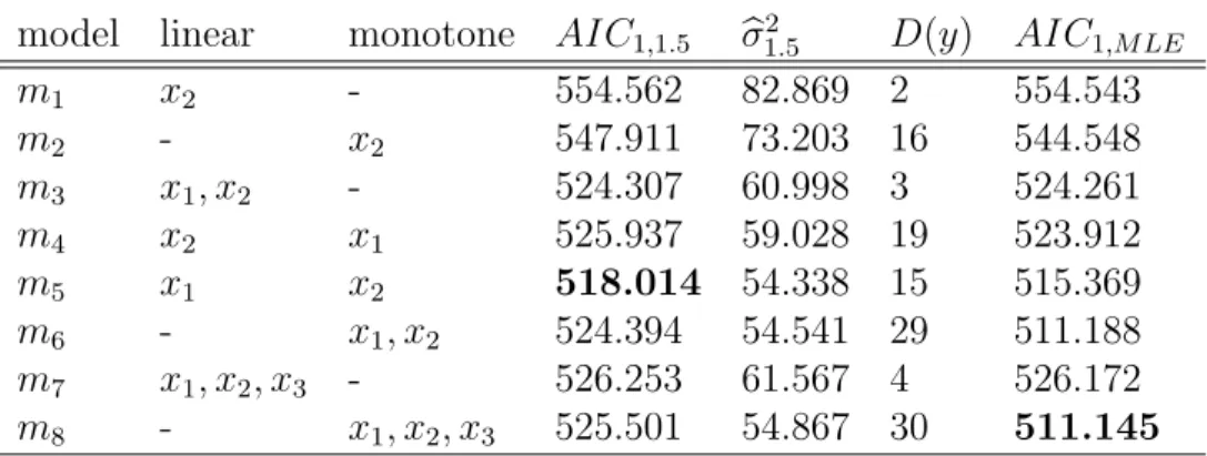
Eight candidate models has been considered according to how the auxil-iary information is used to obtain the estimators. Other models have been discarded as they give clearly worse fits. The description of the models is given in table 1, within the values of AIC1,1.5, bσ

2

1.5,D(y), and AIC1,M LE.

From the AIC1,1.5 values in table 5, the model m5, which includes x1 in a linear form and x2 in a nonparametric form with 15 degrees of freedom and _bσ = 7.37, is selected. It is interesting to note that using AIC1,M LE

the most complex model which includes the three explanatory variables in a nonparametric form, would have been selected. This fact agrees with the conclusions following the simulation results, that AIC1,M LE favors the more

complex models.

model linear monotone AIC1,1.5 bσ

2

1.5 D(y) AIC1,M LE

m1 x2 - 554.562 82.869 2 554.543

m2 - x2 547.911 73.203 16 544.548

m3 x1, x2 - 524.307 60.998 3 524.261

m4 x2 x1 525.937 59.028 19 523.912

m5 x1 x2 518.014 54.338 15 515.369

m6 - x1, x2 524.394 54.541 29 511.188

m7 x1, x2, x3 - 526.253 61.567 4 526.172

m8 - x1, x2, x3 525.501 54.867 30 511.145 Table 5: Model description and fitting results with the Prestige data.

tries to choose between parametric and nonparametric alternatives has been used.

5. Conclusions and future research

The problem of the derivation of the degrees of freedom,DK(y), for

semi-parametric monotone models has been solved. This quantity is incorporate in new AIC measures and in the estimators for the variance parameter, which are shown to be useful in model selection. Besides,DK(y) is also useful to

de-rive inferential tools as hypothesis tests in nested models which is a question to be dealt with in our future research.

It has been shown, by simulation experiments and in the example, that semiparametric models compares favorably with linear alternatives, being the fitting and model selection steps easily achieved. For researchers who dislike the non continuity of the monotone fitted curve with the cyclic PAVA, the consideration of a two-step fitting process is proposed. In a first step, the linear and nonparametric terms defining the model are determined with the

AIC1,1.5 and, in the second step, the nonparametric modeling is performed using alternative approaches, following the researcher’s preferences. Within these alternatives is a hybrid approach that produces monotone estimators, with properties similar to those of nonparametric regression estimators apply-ing a smoother to each monotone component obtained from the backfittapply-ing algorithm (for details see Mukerjee(1988)).

The first extension is the semiparametric additive mixed model:

yi =α+ p

X

j=1

βjxji+ q

X

j=1

hj(zji) +u+εi,

where u ∼ N(0, σ_u2) is a random effect. Rueda et al. (2010), deal with this type of model, when p = 0 and q = 1, to solve small area estimation problems.

The second extension is the general isotonic model where the monotone restrictions are replaced by more general shape restrictions, including concave relationships among others. An interesting reference dealing with isotonic regression models is Meyer (2008), where univariate shape models (p = 0 and q = 1) are studied.

6. APPENDIX

6.1. Proof of lemma 2.1

(i) A polyhedral cone, K, is one that can be defined by a set of lin-ear inequalities: K = {u∈ <n_/a0

iu≤0, i= 1, ..., m}. Let us denote by

span+_{b

1, ..., bs}the subset of <n defined by the non negative linear

combi-nations of {b1, ..., bs}.

It is a known result (Goldman and Tucker (1956)) that a convex cone

C is a polyhedral cone, if and only if, it is finitely generated (with positive coefficients) by a finite number of vectors, that is:

∃a1, ..., am :C ={u∈ <n/a0iu≤0, i= 1, ..., m}

⇔ ∃b1, ..., bs :C=

(

u∈ <n/u=

s

X

i=1

αibi, αi >0

)

=span+{b1, ..., bs}.

Therefore, asCjare polyhedral cones, we have that,Cj =span+

bj1, ..., bjsj , j =

1, ..., q, also, as L is a subspace, ∃ {d1, ..., dl} such as L=span{d1, ..., dl}=

span+_{d

1, ..., dl}+span+{−d1, ...,−dl}. Then, K = span+{b11, ..., b1s1}+

...+span+bq1, ..., bqsq +span

+_{d

1, ..., dl}+span+{−d1, ...,−dl} is also a

(ii) let y ∈ C, p(y/L⊥) = y −p(y/L) ∈ C because L ⊂ C. Then,

p(y/L⊥) = p(y/L⊥∩C) and y=p(y/L) +p(y/L⊥∩C) ∈ L+L⊥∩C. We have proven: C⊂L+L⊥∩C.

The opposite is also true asL⊂C.

Now, lety ∈ <n_{, p(y/C) = p(p(y/C)/L)+p(p(y/C)/L}⊥_{) where,p(p(y/C)/L}⊥₎

=p(y/C)−p(p(y/C)/L)∈C, because L⊂C. Then,

p(p(y/C)/L⊥) =p(p(y/C)/L⊥∩C) and p(y/C) = p(p(y/C)/L)+p(p(y/C)/L⊥∩C) Moreover, from lemma 2.2 in Raubertas (1986),

p(p(y/C)/L) = p(y/L) and p(p(y/C)/L⊥∩C) = p(y/C∩L⊥) and (ii) follows.

(iii) From (ii), as L ⊂L+C, we have that: L+C =L+ (L+C)∩L⊥

and

p(y/L+C) =p(y/L) +p(y/(L+C)∩L⊥) and the result follows.

6.2. Proof of lemma 2.2

(i) To prove the result several properties of projections onto polyhedral cones will be used (see Meyer(1999) and references therein). From lemma 2.1 (ii), K =L0+S1+...+Sq =L0+ ((L0+S1+...+Sq)∩L⊥0) = L0+K0, whereK0 = (L0+S1+...+Sq)∩L⊥0 and dim(L0) =p+ 1.Also, from Lemma 2.1(iii),

p(y/K) =p(y/L0) +p(y/K0) (5) and DK(y) = p+ 1 +DK0(y).

Now, from lemma 2.1(i), K0 is polyhedral and then, K0 is defined by a subset of generators, as follows,

∃ {δi, i= 1, ..., M} ⊂L⊥0 :K0 =span+{δi, i= 1, ..., M}=

(

u∈L⊥₀/u=

M

X

i=1

biδi, bi ≥0

)

and also by a subset of inequality restrictions:

∃ {γj, j = 1, ..., m} ⊂L⊥0 :K0 =

where span+_{γ

j, j = 1, ..., m}=K0p∩L

⊥

0.

Moreover, from proposition 3 in Meyer(1999), for each y ∈ L⊥₀ we can define the sets Iy ⊂ {1, ..., M}, Jy ⊂ {1, .., m} and the corresponding sub-spaces : L(Iy_{) = span{δ}

i, i∈Iy}, L(Jy) =span{γj, j ∈Jy}such as:

p(y/K0) =p(y/L(Iy)), p(y/K

p

0) =p(y/L(Jy)) (6) and

L(Iy)⊥∩L⊥₀ =L(Jy), L(Iy) = (L(Jy))⊥∩L⊥₀. (7) On the other hand, let be θb_j, j = 0,1, ..., q a sequence given by the

back-fitting algorithm, we have that:

p(y/K) = bθ₀+θb₁+...+bθ_q,bθ₀ ∈L₀,bθ_i ∈S_j.

Let vi

j, i = 1, ..., n−1;j = 1, ...q be the generators of the order cones,

then, Sj = span+

vi

j, i= 1, ..., n−1 . Now, for each y ∈ <n and each θb_j,

there exists a set of indexes I_jy such as Ly_j = spanvi_j, i∈I_jy determine

F_jy = Ly_j ∩Sj, which is the face of the cone Sj that has bθ_j as an interior

point. Then, necessarily,

b

θj =

X

i∈I_jy

λijvji, λij >0,∀i, j. (8)

Moreover, from (5) and lemma 2.2 in Raubertas (1986), we have that:

p(y/K) = p(y/L0) +p(y/K0) = θb=p(θ/Lb ₀) +p(θ/Kb ₀) =p(y/L₀) +p(θ/Kb ₀) =⇒

p(y/K0) = p(θ/Kb ₀) =θb−p(θ/Lb ₀) =θb₁+...+bθ_q−p(θb₁+...+θb_q/L₀).

Now, from the last equality, (5), and (8) we have that,

p(y/K0) =

q

X

j=1

X

i∈I_jy

λijvij− q

X

j=1

X

i∈I_jy

λijviLj = q

X

j=1

X

i∈I_jy

λijvjiK,

where, for each iand j, v_ji =viL_j +v_jiK, vi_j ∈K, v_jiL ∈L0, vjiK ∈K0. Now, from (6) and (7) it follows,

∀l∈L(Jy_{), 0 =γ}0

lp(y/K0) =

q

P

j=1

P

i∈I_jy

However, λji > 0 from (8), and γl0vjiK ≤ 0,∀i ∈ I y

j, j = 1, ..., q, l ∈ Jy

(from the definition of K0,) which implies, γj0vjiK = 0,∀i∈I y j, j ∈J

y_{, l∈J}y_.

This last property and (7) imply that,

viK_j ∈ (L(Jy))⊥∩L⊥₀,∀i∈I_jy, j ∈Jy ⇒viK_j ∈L(Iy),∀i∈I_jy, j ∈Jy

⇒ v_ji =v_jiL+v_jiK ∈L0+L(Iy),∀i∈Ijy, j ∈J y_.

Thus, we have proven that,

L0+Ly1+...+Lqy ⊂L0+L(Iy). (9) Now, from the equality p(y/K) = p(p(y/K)/L0 +Ly1+...+Lyq), which is a

consequence of p(y/K) ∈ L0 +Ly1 +...+Lyq, obtained from the backfitting

algorithm, and the statements (5) and (6) we have that,

p(y/K) = p(p(y/K)/L0+L

y

1 +...+L

y

q) =p(p(y/L0) +p(y/K0)/L0 +L

y

1 +...+L

y q)

=p(p(y/L0) +p(y/L(Iy))/L0+L

y

1 +...+Lyq).

Finally, this last statement, the fact that L0 and L(Iy) are orthogonal sub-spaces and (9) imply:

p(y/K) = p(p(y/L0+L(Iy))/L0+Ly1+...+L

y

q) =p(y/L0+Ly1 +...+L

y q)

and the result follows.

(ii) The subspaces associated with faces of order cones have the following general expression:

L={u∈ <n_/u

k =ul,(k, l)∈P},where P ⊂ {(k, l), k = 1, ..., n;l = 1, ..n}.

Let u0 be any vector belonging to L with a maximal number of different components. Let us denote this number by N and let us denote the different values by {u0i}N_i=1. Then, N =dim(L) and a minimal set of generators for

L is given by the set {vi}N_i=1, where:

v_ki = 1⇐⇒u0k =u0i;vki = 0⇐⇒u0k6=u0i, k = 1, ..., n.

Now, the subspace associated with the face containing θb_j as an

inte-rior point is defined as follows: Ly_j = u∈ <n_/u

P_jy =n(k, l)/θb_jk =θb_jl, k, l∈ {1, ..., n} o

. θb_j is a vector belonging to Ly_j with

a maximal number of different components (otherwise other case θb_j would

not be an interior point of the corresponding face). Moreover, if{ajk} Nj

k=1 are the values of the Nj different components of θb_j, then dim(Ly_j) = N_j and a

minimal set of generators for Ly_j is given by the set

vi j

Nj,

i=1 where,

v_jki = 1⇐⇒θb_jk =a_ji;vi_jk = 0 ⇐⇒θb_jk 6=a_ji, k= 1, ..., n

and the result follows.

6.3. Proof of lemma 3.1

The proof follows the same steps to close result close to that found in the paper by Meyer and Woodofre(2000). From Stein’s (1981) identity:

E y−bθC

2

=Eky−θk2−2E < y−θ,θb_C −θ >+E θbC −θ

2 =

=nσ2−2σ2EDC(y) +E

bθC−θ

2

. (10)

Now, from lemma 2.1(iii), and the orthogonality betweenLand L⊥ , we have that:

E

θ−θbC

2

=Ekp(θ/L)−p(y/L)k2+ +Ep(θ/(L+C₀)∩L⊥)−p(y/(L+C₀)∩L⊥)

2

≥rσ2. (11) Moreover, from properties of projections and the Stein identity again:

0≤E < y−bθ_C,θb_C −θ >=E < y−θ,θb_C −θ >−E θbC −θ

2 =

=σ2ED(y)−E

θbC −θ

2

. (12)

Now, from (10)and (11) we have that:

E

y−θbC

2

and from (10)and (12) we have that:

E

y−bθC

2

σ2 ≤n−ED(y) =n−(ED(y)−r)−r. (14) Then, the result follows from (13) and (14).

Acknowledgements: This research was partially supported by Spanish DGES (grant MTM 2009-11161).

[1] Akaike, H. (1973). Information Theory and the extension of the maxi-mum likelihood principle. In: Petrov, B. N., Csaki, F. (Eds), Proceed-ings of the Second International Symposium on Information Theory. Akademiai Kiado, Budapest, pp. 267-281.

[2] Anraku, K. (1999). An information criterion for parameters under a simple order restriction. Biometrika., 86, pp. 141-152.

[3] Bachettti, P. (1989). Additive isotonic models. J. Amer. Statist. Assoc., 84, pp.289-294.

[4] Borra,S. Di Ciaccio, A. (2002). Improving nonparametric regression methods by bagging and boosting. Comp. Stat. Data. An., 38 pp. 407-420

[5] Brunk, H.D. (1970). Estimation of isotonic regression (with discussion). In: Puri, M.L. (Ed). Nonparametric Techniques in Statistical Inference. Cambridge University Press, Cambridge.

[6] Cheng, G. (2009). Semiparametric additive isotonic regression. J. Stat.Plan.Infer., 130, pp. 1980-1991.

[7] Curtis, M. S. and Ghosal, S. (2010). Fast Bayesian Mod

el Assessment for Nonparametric Additive Regression. www4.stat.ncsu.edu/ ghoshal/papers/BayesVarSel.pdf

[8] De Boer, W.J., Besten, P.J. and Ter Braak, C. F. (2002). Statistical analysis of sediment toxicity by additive monotone regession splines.

[9] Dykstra, R. (1983). An algorithm for restricted least squares regression.

Ann.Statist., 3, pp. 401-421.

[10] Fox, J. (1997). Applied regression analysis, linear models and related methods. Sage Publications, McMaster. University, Hamilton, Ontario, Canada.

[11] Goldman, A.J. and Tucker, A. W. (1956). Polyhedral convex cones.Ann. of Math. Studies., 38, pp. 19-40.

[12] Griffin, J.E. and Steel, M.F.J. (2010). Bayesian nonparametric modelling with the Dirichlet process regression smoother. Stat. Sinica. (forthcom-ing).

[13] Hanson, D.L., Pledger, G. and Wright, F.T. (1973). On consistency in monotonic regression. Ann.Statist., 3, pp. 401-421.

[14] Hastie, T. and Tibshirani, R. (1986). Generalized additive models.

Statist.Sci., 3, pp. 297-310.

[15] Huang, J. (2002). A note on estimating a partly linear model under monotonicity constraints. J. Stat.Plan.Infer., 107, pp. 345-351.

[16] Hussian, M., Grimvall, A., Burdakov, O. and Sysoev, O. (2004). Mono-tonic regression for assessment of trends in environmental quality data.

ECCOMAS 2004. P. Neittaanm¨aki, T. Rossi, K. Majava, and O. Piron-neau (eds.). V. Capasso and W. J¨ager (assoc. eds.). Jyv¨askyl¨a.

[17] Kato, K. (2009). On the degrees of freedom in shrinkage estimation. J. Multivariate Anal., 100, pp. 1338-1352.

[18] Li, R. and Liang, H. (2008). Variable selection in semiparametric regres-sion modeling. Ann. Statist., 36, pp. 261-286.

[19] Liu, T., Lin, N., Shi, N. and Zhang, R.(2009). Information criterion-based clustering with order-restricted candidate profiles in short time-course microarray experiments. Bioinformatics., 10:146.

[21] Meyer, M. (1999). An extension of the mixed primal-dual bases algorithm to the case of more constraints than dimensions. J. Stat.Plan.Infer., 81, pp. 13-31.

[22] Meyer, M. and Woodrofe, M. (2000). On the degrees of freedom in shape-restricted regression. Ann.Statist., 28, pp. 1083-1104.

[23] Meyer, M. (2008). Inference using Shape-restricted regression Splines.

Ann.Statist., 2, pp. 1013-1033.

[24] Morton-Jones, T., Diggle, P., Parker, L., Dickinson, H.O. and Binks, K.(2000). Additive isotonic regression models in epidemiology.

Stat.Med.,9, pp. 849-59.

[25] Mukerjee, H. (1988). Monotone nonparametric regression.

Ann.Statist.,16, pp. 741-750.

[26] Raubertas, R.F., Lee C.C. and Nordheim, E.V. (1986). Hypothesis Test for normal means constrained by linear inequalities. Commun.Statisti.-Theor.Meth., 15, pp. 2809-2833.

[27] Robertson, T., Wright, F.T., Dykstra, R.L. (1988). Order Restricted Statistical Inference. Wiley.

[28] Rueda, C., Men´endez, J.A. and Gomez, F. (2010). Small Area Estima-tors based on restricted Mixed models. TEST., 19, pp. 558-579.

[29] Sampson, A. R., Singh, H. and Whitaker, L.R. (2003). Order restricted estimators: some bias results. Stat.Probabil.Lett., 61, pp. 299-308. [30] Stein, C. (1981). Estimation of the mean of a multivariate normal

dis-tribution. Ann.Statist., 9, 1135-1151.

[31] Stone,C.J. (1982). Optimal Global rates of convergence for nonparamet-ric regression.Ann.Statist., 10, 1040-1053.

[32] Stone,C.J. (1982). Additive Regression and other nonparametric mod-els.Ann.Statist., 13, 689-705.

[34] Zhao, L. and Peng, L. (2002). Model selection under order restrictions.

Stat.Probabil.Lett., 57, pp. 301-306.