C
C
|
E
E
|
D
D
|
L
L
|
A
A
|
S
S
Centro de Estudios
Distributivos, Laborales y Sociales
Maestría en Economía Universidad Nacional de La Plata
Growth and Income Poverty in Latin America and
the Caribbean: Evidence from Household Surveys
Leonardo Gasparini, Federico Gutiérrez y Leopoldo
Tornarolli
Documento de Trabajo Nro. 30
Diciembre, 2005
Growth and Income Poverty
in Latin America and the Caribbean:
Evidence from Household Surveys
*Leonardo Gasparini**
Federico Gutiérrez
Leopoldo Tornarolli
CEDLAS***
Universidad Nacional de La Plata
Abstract
This paper provides evidence on growth and income poverty in Latin America and the Caribbean (LAC). Results are obtained by processing microdata from household surveys of 18 LAC countries covering the 1990s and early 2000s. Over this period the LAC economies experienced very heterogeneous patterns of growth and poverty changes. Most countries in the region had a rather meager performance in terms of poverty reduction. Episodes of positive, significant and unambiguously pro-poor income growth have been rare in Latin America.
Keywords: poverty, growth, inequality, pro-poor growth, Latin America.
* This paper started as a contribution to the 2005 World Bank LAC Flagship Report,
Virtuous Circles of
Poverty Reduction and Growth. We are very grateful to the encouragement and comments of Omar Arias,
Humberto López and Jaime Saavedra. All the statistics were computed at CEDLAS-UNLP. We are grateful to Georgina Pizzolitto, Francisco Haimovich, Victoria Fazio, Julieta Pron, Ana Pacheco, Monserrat Bustelo, Carolina García Domench, Hernán Winkler, Matías Horenstein, Evelyn Vezza, Javier Ibarlucia, Elena Cadelli, Rocío Carbajal, Sergio Olivieri, Gimena Ferreyra and Rafael Brigo for outstanding research assistance. We are also grateful to Martín Cicowiez for comments and assistance, and two anonymous referees for valuable suggestions. The usual disclaimer applies.
** Corresponding author. E-mail: leonardo@depeco.econo.unlp.edu.ar
*** CEDLAS is the Center for Distributional, Labor and Social Studies at Universidad Nacional de La Plata
1. Introduction
The empirical literature on growth and poverty has flourished since the late 1990s. Based on household survey microdata, several contributions have tried to elucidate whether
economic growth tends to “lift all boats”, in particular those of the poor.1 The concern for
pro-poor growth is in part the consequence of evidence showing that in some countries the fruits of economic growth were not equally shared by all the population, and, more worrisome, evidence that in some growth episodes the well-being of the poor actually decreased.
This paper provides evidence on pro-poor growth for a sample of 18 Latin American and Caribbean (LAC) countries in the period 1989-2004. Assessing whether growth is associated to a sizeable reduction in poverty is a relevant issue everywhere, but it is particular so in Latin America, a region with arguably the highest levels of inequality in the world, and where the economic reforms that allowed most countries to grow since the early 1990s are still a hot issue of debate.
The literature on poverty and pro-poor growth in Latin America is comprised by two types of studies. On the one hand, there is a large number of country studies providing evidence
on poverty and growth patterns for a given economy.2 Although these contributions can be
combined to get an overall picture for Latin America, the conclusions from this merge may be weak, since country studies significantly differ in many dimensions: the welfare indicator (income or consumption), the poverty line, the time period, and the statistics shown. They surely also differ in the hundreds of small decisions needed to get from the raw data to a poverty estimate (zero incomes, outliers, missing data, weights, and so on).
1 Adelman and Morris (1973) and Ahluwalia (1976) are early contributions to this literature. The recent
contributions include Ravallion and Chen (1997), Baulch and McCullock (2000), Dollar and Kraay (2000), Kakwani and Pernia (2000), Morley (2001), Foster and Székely (2001), Ravallion and Chen (2003), Kakwani and Son (2004), López and Servén (2004), Ravallion (2004) and Son (2004), among others. Several recent World Bank Poverty Assessments include discussions and evidence on pro-poor growth at the country level.
2 The relevant country-specific papers are too many to fit in the typical space of a footnote. See World Bank
The second strand of the literature tries to alleviate these problems by processing household surveys from many countries with a consistent methodology. The main international organizations in the region (Inter-American Development Bank (IADB), United Nations (through CEPAL), and the World Bank) have produced poverty and inequality studies
including several countries.3 This paper differs from that literature in two dimensions. On
the one hand, we use a larger and more updated dataset than previous studies, and provide a more detailed explanation of the methodology to make the statistics comparable. More importantly, to the best of our knowledge this is the first paper in which a large consistent dataset of Latin American household surveys is used to compute and analyze a broad set of pro-poor growth measures. While previous studies are restricted to the traditional poverty and inequality estimates, this paper adds several indicators of pro-poor growth. By computing pro-poor growth rates, poverty equivalent growth rates, poverty-growth elasticities, growth-incidence curves and isopoverty curves with alternative poverty lines for all Latin American countries based on a large set of household surveys processed with a consistent well-documented methodology, we are able to provide a more rigorous and comprehensive picture of poverty and pro-poor growth in the region than the previous literature.
The results of the paper suggest a strong correlation between economic growth and income poverty reduction at the country level. On average, poverty has just slightly fallen in Latin America and the Caribbean since the early 1990s due to slow income growth (when income is measured with household survey data) and increases in inequality. The evidence shown in the paper suggests a remarkable heterogeneity of growth and poverty reduction patterns across LAC countries. However, almost none of these economies experienced sustainable strong growth along with significant equalizing distributional changes in the period 1989-2004. By means of microsimulations we illustrate the efforts in terms of neutral growth and simple redistributive policies needed by each LAC country to attain certain poverty-reduction targets. These efforts, sizeable in most countries, depend on the shape and central position of the income distribution.
3 See Altimir (1994, 1996), Attanasio and Székely (2001), Behrman
et al. (2002), CEPAL (2005), Fields
The rest of this paper is organized as follows. In section 2 we briefly introduce the dataset and the main methodological issues involved in measuring growth and income poverty. Section 3 starts with a basic question: have Latin American and the Caribbean countries grown in the last 15 years? In section 4 we study the distribution of growth rates across income strata by examining growth-incidence curves. Section 5 restricts the analysis to the lower tail of the income distribution. We compute measures of income poverty, and analyze whether growth has been associated to a reduction in the proportion of poor people in the population. Section 6 focuses not on the number of poor people, but on their incomes: has growth been associated to an increase in the incomes of the poor? We also study whether income growth has been higher or lower in poor strata compared to the rest of the population. The links between poverty, growth and inequality in the recent experiences of LAC economies are examined in section 7 by means of microsimulations. We also compute different configurations of neutral growth rates and redistributive policies needed to achieve certain poverty reduction targets. Section 8 closes with some concluding remarks.
2. The data
Most of the statistics in this paper are obtained by processing microdata from household surveys, and are part of the Socioeconomic Database for Latin America and the Caribbean (SEDLAC), jointly developed by CEDLAS at the Universidad Nacional de La Plata (Argentina) and the World Bank’s LAC poverty group (LCSPP). The SEDLAC contains information on more than 150 household surveys in 21 LAC countries. In this paper we restrict the sample to 57 household surveys carried out in 18 LAC countries during the 1990s and early 2000s (see Table A at the end of the paper). The sample includes data for Argentina, Bolivia, Brazil, Chile, Colombia, Costa Rica, Dominican Republic, Ecuador, El Salvador, Honduras, Jamaica, Mexico, Nicaragua, Panama, Paraguay, Peru, Uruguay and Venezuela. The sample covers all countries in mainland Latin America (except for Guatemala), and two of the largest countries in the Caribbean (Dominican Republic and Jamaica). For most countries our sample has three observations corresponding to the early
and mid 1990s, and the early 2000s. In each period the sample represents around 92% of LAC total population (98% in Latin America and 29% in the Caribbean). Most household surveys included in the sample are nationally representative. The two exceptions are Argentina and Uruguay, where surveys cover only urban population, which nonetheless
represents more than 85% of the total population in both countries.4
Most Latin American countries have experienced significant improvements in their household surveys in the last decades. In particular, major changes have been implemented in several LAC countries since mid 1990s after the implementation of the MECOVI Program. Although these changes are welcome, they pose significant comparison problems. An example of this situation is the increase in the geographical coverage of the survey. Since regions differ in their economic and social situations, adding a new region into the survey usually significantly affects the national statistics. In countries where changes in geographical coverage of the survey occurred we provide ways of assessing the impact of those changes. For instance, in Bolivia the household survey was urban in 1993 and nationally representative in 1997. We present two sets of statistics for Bolivia 1997: one for the whole sample and one only for those urban areas also surveyed in 1993.
Household surveys are not uniform across LAC countries. The issue of comparability is of a great concern. We have made an effort to make statistics comparable across countries and over time by using similar definitions of variables in each country/year, and by applying consistent methods of processing the data. However, perfect comparability is far from being assured. A trade-off between accuracy and coverage arises. The particular solution adopted contains an unavoidable degree of arbitrariness. We tried to be ambitious enough to include all countries in the analysis, and accurate enough so not to push the comparisons too much. In any case, we provide the reader with relevant information to assess the trade-offs
throughout this paper, and in the guide of the dataset in the SEDLAC webpage.5 That guide
4 Some studies suggest that including rural areas would not substantially affect poverty estimates in these two
Southern Cone countries (Haimovich and Winkler, 2005; Winkler, 2005). Some LAC countries introduced national household surveys in the mid 1990s. For time comparison purposes in some cases we restrict the analysis to urban areas (e.g. Colombia), despite the availability of recent national surveys.
is a companion document to this paper, and should be helpful to those interested in technical details.
We perform the poverty and pro-poor growth analysis using four alternative poverty lines: the international lines of USD 1 and USD 2 a day at PPP, and the moderate and extreme poverty lines used by national governments in each country. For the latter we replicate, whenever possible, the income/consumption variable used by the National Statistical
Offices (NSO) to compute official poverty estimates in each country.6 In most cases it is an
income variable, although in some cases (e.g. Mexico and Peru) it implies computing a
consumption aggregate. These national “income” variables widely vary across countries, as they differ in the treatment of adult equivalent scales, regional prices, implicit rent from own housing, zero incomes, adjustments for non-response and misreporting, and other issues.
In contrast, to apply the international lines of USD 1 and USD 2 we construct a homogeneous household per capita income variable across countries/years that includes all the typical sources of current income. In the web site of the SEDLAC we include tables with all the items considered (or excluded) to compute a comparable income variable in
each country/year.7
It is well known that household consumption is a better proxy for well-being than
household income.8 Despite this dominance, nearly all comparative distributional and
poverty studies in LAC use income as the well-being indicator. A simple reason justifies this practice: few countries in the region routinely conduct national household surveys with consumption/expenditures-based questionnaires, while all of them include questions on individual and household income. Some authors and agencies adjust average income to accord with consumption data from National Accounts to estimate poverty (CEPAL, 2003;
Wodon et al., 2000; WDI, 2002). However, it is not clear that the adjustment for
6 In those countries where there is not a national agency estimating poverty we either follow a World Bank
Poverty Assessment or some well-know country study. In Brazil, for instance, we follow the methodology proposed by Barros, Carvalho and Franco (2004).
7 See www.depeco.econo.unlp.edu.ar/cedlas/sedlac
consumption increases comparability, since the reliability of National Accounts need not be greater than the reliability of household surveys. Deaton (2003) strongly argues for the use of only survey data to compute poverty, as adjustments to match National Accounts “tend to overstate the reduction of poverty over time, and to exaggerate poverty differences across countries”. In this paper we do not perform any adjustment to compute poverty from household surveys. WDI (2003) reports that poverty measures based on consumption and those based on income without adjustment do not significantly differ, due to two effects that roughly cancel each other out: mean income is higher than mean consumption, but income inequality is higher than consumption inequality. Since 2003 the WDI reports poverty statistics computed without adjusting income to match consumption from National Accounts.
Most household surveys report incomes obtained during the month previous to the survey.
Some surveys also include information on incomes earned in the last six months (e.g.
ENIGH in Mexico). In those cases, and for comparative purposes, we only include incomes earned in the last month. Incomes are transformed into monthly incomes if values are not
reported on a monthly basis (e.g. weekly payments).
We apply consistent rules to deal with missing incomes. Suppose income from source s is
missing for individual i. Should we record as missing that individual’s total income? If we
take that alternative, should we in turn record as missing the total income of individual i´s
household? We make the following (necessarily arbitrary) decisions. If s is not the main
source of income for i, then we compute the individual total income ignoring source s.9If
instead s is the main source, we record total income as missing. This alternative has the
advantage of not dropping from the dataset individuals who do not respond questions on income sources of secondary importance. The cost to be paid is the likely income under-estimation for these individuals. Regarding household income, we record it as missing if the household head’s total income is missing. Otherwise, we compute household income assigning zero income to non-heads with missing income.
Our household income variable includes an estimate of the implicit rent from own housing. Some surveys include reliable self-reports of the implicit rent. In those surveys where this information is not available, or is clearly unreliable, we increase household income of housing owners by 10%, a value that is consistent with estimates of implicit rents in the region. All rural incomes are increased by a factor of 15% to capture differences in rural-urban prices. That value is an average of a set of detailed studies of regional prices in the region (Gasparini, 2007). Although certainly arbitrary, we believe this alternative is better than (i) ignoring the problem of regional prices altogether, or (ii) using for each country the available price information, despite the enormous differences in methodology, scope, and results.
3. Growth: evidence on the mean
The region had a positive but modest performance in terms of per capita GDP growth between 1990 and 2004. The unweighted average annual growth rate was 1.3% when GDP is measured in real local currency units (LCU), and 1.4% when GDP is measured in PPP US dollars (adjusted by the implicit price deflator of GDP in the United States). Most countries in the region managed to grow. However, per capita GDP growth rates were rather modest: only a few countries grew at more than 3% per year. Around half of the countries in the region had disappointing rates of less than 1%. Growth was not uniform across regions and over time (see Table 1). After a bad performance during the 1980s (“the lost decade” in terms of growth), the LAC economies grew on average at around 2% in the 1990s fueled by favorable external conditions and market-oriented reforms. The region suffered a period of slower growth and recessions in the early 2000s, with deep crisis in
some countries. The mean growth rate was a negligible 0.1% in the period 2000-2004.10
- Place Table 1 here –
10 Since around 2003 most countries have overcome the crisis and started to grow again at relatively high
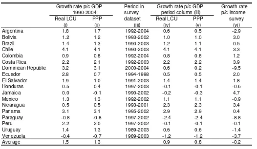
Table 2 shows the annual growth rates for the countries included in this study. The unweighted average growth rate in the sample is 1.5% when measured in real LCU. Unfortunately, our analysis with survey microdata does not cover exactly the period 1990-2004 in each country. That mismatch is driven mainly by the unavailability of reasonably comparable household surveys in both years. Columns (iv) and (v) in Table 2 show the annual per capita GDP growth rates for the periods to be analyzed with the available household surveys in each country. On average the growth rates are somewhat smaller, mainly because for some countries our sample starts in the mid 1990s.
- Place Table 2 here –
Column (vi) in Table 2 reports the annual growth rates in our homogeneous household per
capita income variable computed from household survey microdata.11 Growth in that
variable does not coincide with per capita GDP growth from National Accounts. Of course, they are two different concepts and there are many reasons why they may differ in practice. The linear correlation coefficient between growth rates in household surveys and in per capita GDP is positive and significant. However, some of the differences seem very large. In five countries the sign of the growth rates are different. Since poverty figures are drawn from household surveys, recorded poverty trends may be different from what is expected from looking at per capita GDP figures. Given that, should we adjust incomes in household surveys to match National Accounts? There are good arguments to avoid the adjusting, at least until differences in National Accounts and household surveys are well-understood (Deaton, 2005). A careful study of the reasons behind the differences would be extremely helpful, but it is beyond the scope of this paper. In section 5 we include poverty estimates obtained by adjusting mean income by National Accounts to provide a robustness check to our calculations.
11 In Chile incomes from household survey are adjusted to match some National Accounts figures.
4. Growth: evidence on its distribution
The growth-incidence curves introduced by Ravallion and Chen (2003) are simple and illustrative instruments to analyze growth rates along the income distribution. Specifically, they show the proportional income change at each percentile of the income distribution. They are frequently used to study the extent to which different segments of the population participate in the growth process (or suffer from a recession). The interpretation of such a simple instrument, however, should be made with caution. There are multiple factors that affect income changes, and all are reflected at the same time in a growth-incidence curve. Some of them may have nothing to do with the “growth process”, and some may have complex interactions. Suppose half of the population lives in the countryside and is poor, while the other half lives in the cities and is not poor. Suppose in a given period the government has made investments in schools and infrastructure that allowed productivity to increase 50% in rural areas and 20% in urban areas. However, in the same period the international price of the main crop collapsed, reducing the price received by local farmers by 50%. In that scenario, the growth-incidence curve for the country might show stagnant incomes for the poor, and increasing incomes for the non-poor. Growth in this country is then typically characterized as “not pro-poor” in any of its definitions, despite the fact the increase in productivity driven by the government policies benefited (especially) the poor.
Figures 1 show the growth-incidence curves for all the countries in our sample. These curves are constructed from the household per capita income variable obtained in each
country using the common methodology.12 These curves are known to be very volatile at
the extremes, especially in the bottom percentiles. For this reason we have computed confidence intervals, and deleted from the figures those points where estimates seem very
imprecise.13 A disappointing result should be noticed from the outset: almost none of the
LAC countries experienced sustainable strong growth along with significant equalizing distributional changes. In fact, Nicaragua is the only country where the growth-incidence
12 Growth-incidence curves for the income/consumption variables used for the estimation of official poverty
with national lines are available from the authors upon request.
curve lies above the horizontal axis and is decreasing on income, that is, economic changes have benefited all the population, and particularly the poor.
- Place Figure 1 here –
The figures illustrate the heterogeneous growth patterns experienced by the LAC countries over the last 15 years. For instance, in the Southern Cone, while Chile has experienced sustainable growth along the income distribution, in Argentina income changes have been negative and clearly unequalizing. Although to a lesser extent, that was also the pattern for Uruguay. In contrast, between 1990 and 2003 incomes in Brazil increased a bit, in particular in the first half of the 1990s. The growth-incidence curve of Figure 1 suggests mild equalizing income changes in that country.
5. Growth and poverty I: the proportion of poor people
As an economy grows incomes go up, and then it is expected that some people are able to jump out of poverty. The relationship between economic growth and income poverty is, however, a subject of much debate. Is there really a negative correlation between these two phenomena? Is the correlation strong? Are there many exceptions to the growth-poverty-reduction story? We start this section by showing poverty statistics, and then link them to growth figures.
The USD1-a-day line was proposed in Ravallion et al. (1991) and used in World Bank (1990). It is a value measured in 1985 international prices and adjusted to local currency using purchasing power parities (PPP) to take into account local prices. The USD 1 standard was chosen as being representative of the national poverty lines found among low-income countries. The line has been recalculated in 1993 PPP terms at $1.0763 a day (Chen and Ravallion, 2001). This value is multiplied by 30.42 to get a monthly poverty line. The USD-2-a-day line is also extensively used in comparisons across middle-income countries (like most of LAC ones), and periodically presented in the World Development Indicators (WDI). Although the USD 1 or 2 lines have been criticized, their simplicity and the lack of reasonable and easy-to-implement alternatives have made them the standard for
international poverty comparisons.14
Following Deaton (2003) and WDI (2004) we compute the poverty line for 1993 in local currency units using the PPP adjustment, and then take that value to the month(s) of a given survey using the national consumer price index of the country.
We also compute moderate and extreme poverty using national lines, whenever possible. Most LAC countries have official national extreme poverty lines which are mostly based on the cost of a basic food bundle, and moderate poverty lines computed from the extreme lines using the Engel/Orshansky ratio of food expenditures. Despite some similarities, methodologies for national poverty estimates substantially differ across nations. Some
countries use expenditures (e.g. Mexico), others use incomes (e.g. Argentina) and others a
mix of income and expenditures (e.g. Bolivia).
5.1. Poverty changes
Has poverty fallen in LAC countries during the last 15 years? The estimates in Table 3 suggest a remarkable heterogeneity. While some countries achieved significant poverty
reductions (e.g. Brazil, Chile, El Salvador, Jamaica, Nicaragua), some others experienced
large increases in the incidence of poverty (e.g. Argentina and Venezuela). Figure 2
14 See Srinivasan (2004), Kakwani (2004) and Ravallion (2004) for a discussion on the merits and demerits of
illustrates these disparities by showing the change in the poverty headcount ratio
(USD-2-a-day poverty line) between the early 1990s and the estimated value for 2004.15 The results
are robust to other poverty indicators.16
- Place Table 3 here –
- Place Figure 2 here –
On average, the Latin American performance in terms of poverty reduction over the last 15 years has been rather disappointing (see Table 4). The population-weighted mean of the poverty headcount ratio has dropped 1.2 points when using the USD-2-a-day line. The fall in the unweighted mean has been larger, but still meager: just less than 2 points. Poverty
moderately fell over the 1990s and increased in the early 2000s.17 As the population has
been growing, and the incidence of poverty did not significantly decay, the number of poor people in the region has increased. The recent recovery of the LAC economies is helping reducing poverty in most countries, but even in that scenario the overall assessment of the last two decades is not positive. Figure 3 shows a small drop in the LAC mean poverty headcount ratio between the early 1990s and 2004, and an increase in the number of poor people, using both the USD 1 and 2 lines.
- Place Table 4 here –
- Place Figure 3 here –
There are substantial differences across regions in poverty reduction. The unweighted poverty mean clearly went down in Central America. In contrast, the performance in South America has been weak, while poverty levels went up in the Andean community. The population-weighted results are somewhat different. As poverty decreased in the most-populated country of the region, Brazil, the poverty weighted-mean in the Mercosur went
15 Year 2004 poverty figures are estimated by combining per capita GDP growth rates with poverty-growth
elasticities (see below). The same procedure is applied when we do not have estimates (own or from other sources) for the early 1990s for a given country.
16 See the SEDLAC webpage for estimations of the FGT(1) and FGT(2) for all country/years.
17 The general picture of poverty trends in Latin America from this paper is similar to that from other sources
significantly down. In contrast, as poverty in Mexico stayed unchanged, the poverty record in Central America appears less impressive when taking weighted means.
As discussed in section 3 changes in incomes from household surveys do not match figures from National Accounts. Although our preferred option is to compute poverty only with data from household surveys, in order to check for robustness we also follow the methodology in Sala-i-Martin (2006) and anchor the mean of the distribution with the per capita GDP of each country. Table 5 reports changes in poverty under the two alternatives. The linear correlation between the two columns is positive and significant (0.78). However, in some countries the differences are sizeable. For instance, while poverty went up 11.4 points in Argentina according to household survey data, the increase is 4.4 points when adjusting the mean for National Accounts figures. In accordance with the findings of Deaton (2003), in most LAC countries poverty falls more (or increases less) when adjusting for GDP growth. That may be due to faster growth of some income sources not common among the poor (capital, benefits, rents). In that case, adjusting incomes in household surveys for GDP growth would overstate the fall in poverty.
- Place Table 5 here –
5.2. Growth and poverty
It is said that growth is a fundamental ingredient in the recipe for poverty reduction. In this section we examine whether growth in mean income was in fact associated to a reduction in the proportion of people below the poverty line, and how strong this link seems to be in Latin America.
- Place Figure 4 here –
The strong empirical relationship shown above could be the result of a tight association between economic development and poverty reduction that occurred in the past, but that no longer exists. In fact, some people argue that the new growth patterns in the globalization era are leaving the poor behind, and that aggregate economic growth is no longer closely linked to poverty reduction. Figure 5, however, suggests that there has been a significant relationship between economic growth and poverty reduction during the last two decades. The linear correlation when using per capita GDP growth rates is -0.62 in panel A and -0.68 in panel B. Notice, however, that those economies that have been stagnant or growing at very low rates (in terms of per capita GDP) have experienced poverty increases: the linear regression line lies above the origin. On average only economies that have grown at more than annual 1% have been able to reduce poverty. The relationship growth-poverty reduction is stronger when considering the annual growth rates in incomes from household surveys: the correlation coefficient is -0.87 in the two bottom scatterplots of Figure 5.
- Place Figure 5 here –
Of course, these simple correlations do not prove any causal relationship. That economic growth is empirically associated to a reduction in poverty does not mean that anything that makes mean income go up will make poverty go down. It also says nothing about the need for policy interventions and the appropriate policy instruments. However, the correlations shown suggest the relevant role that growth should have in any poverty-reduction strategy.
- Place Table 6 here –
In most countries episodes of economic growth are associated to growing disposable income and falling poverty, implying negative poverty-growth elasticities. The magnitude of these elasticities varies as we consider incomes from surveys or GDP from National Accounts, and alternative poverty lines. On average, the elasticity is around -1.4 when considering international poverty lines and income growth from household surveys, and -1.7 when using GDP growth from National Accounts. The results obtained from a cross-country regression are similar (Table 7). The results are just illustrative since we have only 30 observations. The estimated poverty-growth elasticities are around -1.6. The interactions of the growth rate with the distance between the poverty line and the mode of the income distribution, and with the change in the Gini coefficient do not appear to be statistically significant.
- Place Table 7 here –
6. Growth and poverty II: the real and relative incomes of the poor
Frequently, the discussion about growth and poverty deals not with the change in the number of poor people, but with the income changes experienced by the poor. In this section we start by examining changes in real incomes of the poor population, and then turn to relative incomes.
6.1. The real incomes of the poor
According to one well-know definition growth is said to be pro-poor if and only if poor
people benefit in real terms (Ravallion and Chen, 2003; Ravallion, 2004). The growth-incidence curves computed in section 4 are useful instruments to assess changes in the real incomes of the poor. The fact that the curve is above the zero axis at all points up to the
headcount ratio H means that real income has increased for all the poor population.18
where σi are the weights, which are non-increasing in income xi. In a typical poverty
analysis the weights attached to the non-poor are zero, i.e. σi=0 if xi≥z, where z is the
poverty line. In this context growth is said to be pro-poor if α>0. In particular, if σi is the
same for all the poor people an equal to 1/NH, where N stands for total population, then α
is just the average of the growth rates of the poor. Ravallion and Chen (2003) argue for the use of this average as a measure of pro-poor growth. They show that this indicator is equal to the change in the Watts poverty index per unit time divided by the headcount index.
The Ravallion and Chen’s measure of pro-poor growth is computed in Table 8 for all the countries in our sample. In most cases we present the results for four alternatives poverty lines. In columns (iii) and (iv) we compute the mean growth rate of household per capita income for those below the USD1 and USD2 lines, respectively. In columns (v) and (vi) we compute the mean growth rate in the income (or consumption) variable used for official poverty estimates in each country, for those below the extreme and moderate lines. In all
cases we compute growth rates for those percentiles below H in the initial period.
- Place Table 8 here –
The table reads as follows. Between 1992 and 2004 mean income in the Argentina’s Encuesta Permanente de Hogares decreased at an annual 2.9%. The fall in per capita income for the poor was much harsher: around 7.9% per year for the USD 2 a day definition. Real incomes for the most disadvantaged fraction of the Argentine population have decreased at a fast rate.
Pro-poor growth rates have been positive in urban Bolivia, Brazil, Chile, Costa Rica, El Salvador, Jamaica, Panama, and Nicaragua, and negative in Argentina, Colombia, Mexico, Uruguay and Venezuela. Dominican Republic, Ecuador, Honduras and Paraguay also experienced negative pro-poor growth rates since mid 1990s.
6.2. The relative incomes of the poor
It is argued that the concept of pro-poor growth should make reference to situations where growth is associated to a proportionally larger income increase for the poor than for the rest of the population. According to this view growth is pro-poor if poverty falls more than it would have if all incomes had grown at the same rate (Baulch and McCullock, 2000; Kakwani and Pernia, 2000; Kakwani and Son, 2004; Son, 2004).
Perhaps surprisingly, the term progressivity, extensively used in tax and benefit-incidence
analysis, has been rarely used in this literature. A program is said to be progressive if the benefits as a share of income are a decreasing function of income. In the same way, growth
can be defined as progressive if the change in income as a share of initial income (i.e. the
growth rate) is a decreasing function of income. Define β as a weighted sum of the
difference between the individual income growth rate gi and the growth rate of the mean
gµ., i.e. β=∑iσi(gi-gµ). Growth is said to be progressive if β>0. In the case where σi=0 if
xi≥z, and σi=1/NH if xi<z, then β is just the difference between the average of the growth
rates of the poor and the growth rate of the mean. The last panel in Table 8 reports this measure of progressive growth for four alternative poverty lines. The experiences have been heterogeneous across countries. Only four countries have significant progressive growth rates. In the case of Dominican Republic and Paraguay that reflects the fact that the poor suffered less (in terms of income changes) than the non-poor in the recent economic contractions. In Panama and despite a stagnant mean income, the incomes of the poor have increased. Finally, Nicaragua is the only country that exhibits growth rates that are
significant, positive and progressive.19
7. Poverty, growth and inequality: assessing the past and looking to the
future
Driven by a multiplicity of factors individual real incomes change in a given period. These changes usually modify different dimensions of the income distribution, like the mean, the degree of dispersion, and the mass below certain cut-off points. In this sense growth, (associated to the change in the mean of the income distribution), changes in inequality (associated to changes in the income dispersion), and changes in poverty (associated to changes in the lower tail of the distribution) are all particular manifestations of the change in the whole income distribution. Growth, inequality and poverty are “endogenous
variables”, and then it is not valid, for instance, to think changes in poverty as caused by
growth and changes in inequality.
Being said that, researchers have found useful to decompose the change in the whole income distribution into two steps: changes in its central position (growth) and changes in its dispersion (inequality). Each of these steps in turn implies changes in the lower tail of the distribution (poverty). In that analysis, then, changes in poverty are presented as the result of growth and changes in inequality. Growth rates in Latin America were analyzed in the previous sections. In this section we first take a look at inequality, and then discuss the decomposition of poverty changes into growth and redistribution effects.
7.1. Inequality changes
The measurement of inequality faces many conceptual and practical issues that are treated
in a vast literature.20 In Table 9 we show changes in some of the most widespread
inequality indicators computed over the distribution of household per capita income. The SEDLAC web page presents the levels of these inequality measures, estimates using other
19 However, notice that the assessment is not that good when taking consumption as the welfare indicator, that
is, the variable that is used in Nicaragua to compute official poverty with national lines.
20 For practical issues in Latin America see Székely and Hilgert (2000), Gasparini (2004) and World Bank
income variables, and confidence intervals for the Gini coefficients. Although the inequality ranking of countries varies as we consider different indices, the linear correlations among indices are high. Argentina, Costa Rica, Dominican Republic, Uruguay and Venezuela consistently rank as the most equal economies in the region, while Bolivia, Brazil, Ecuador, Panama and Paraguay occupy the last positions in the inequality ladder.
- Place Table 9 here –
The assessment of the changes in inequality becomes more dependent on the index used
(see Table 9).21 The correlations are still positive and significant, but smaller in size than
the correlations of inequality levels. Argentina and Colombia stand out as the countries that experienced the largest increases in inequality, with changes of around 6 Gini points. Bolivia, Costa Rica, Ecuador, Uruguay and Venezuela have also witnessed unequalizing distributional changes. Brazil is the only country for which all indices coincide in reporting a drop in income inequality. In Mexico all measures but the Atkinson index with inequality-aversion parameter 2 suggest a fall in inequality.
7.2. Exploring the changes in poverty
As discussed above, changes in poverty can be statistically decomposed into growth and redistribution effects. In particular, we simulate the poverty change that would have occurred in a given period, had the mean income changed, but the shape of the distribution stayed fixed. In this simulation poverty changes as the “result” of changes in mean income,
while inequality remains unchanged. This is the growth effect on poverty changes. The
redistributioneffect records the change in poverty that would have occurred if the shape of
the distribution had changed in the way it did, but the mean had remained fixed.22 Table 10
shows the results of decomposing poverty changes into growth and redistribution effects
21 In contrast, the assessment does not depend on the income variable used. For instance, the correlation
coefficients of the changes in inequality computed over the distribution of per capita income and over the distribution of household income adjusted for adult equivalent scales are around 0.99.
22 See Mahmoudi (1998). Datt and Ravallion (1992) introduced the poverty-change decompositions using
for each country in our dataset, using four alternative poverty lines. Negative numbers mean that income growth and drops in inequality have contributed to poverty reduction.
- Place Table 10 here –
Poverty as measured by the USD2 line increased 11.9 points in Argentina between 1992 and 2004 (column iv). If all incomes had changed (decreased in the Argentine case) at the same rate as the mean did, then the poverty headcount ratio would have increased 4.3 points (column v). The remaining 7.6 points of poverty increase (column vi) were driven by changes in the shape of the income distribution, which in the Argentine case were unequalizing. Notice that while the redistribution effect accounts for most of the poverty change when using the international and the national extreme lines, the growth effect becomes prominent when using the national moderate poverty line. This observation is mainly driven by the fact that the national moderate poverty line is close to the mode of the income distribution in Argentina.
Most of the successful stories of poverty reduction (using the USD 2 line) were driven by generalized growth: Bolivia (92-03), Chile (90-03), Costa Rica (92-03), El Salvador (91-03), Jamaica (90-02), and Nicaragua (93-01). Only in Brazil (90-03) and Panama (95-02) the redistribution effect was larger than the growth effect. Brazil and El Salvador are the only cases for which both the growth and the redistribution effect were significantly poverty-reducing for all poverty lines.
Unequalizing distributional changes are behind the increase in poverty in Argentina (92-04), Colombia (92-00), and Ecuador (94-98). In contrast, the raise in poverty is mainly or totally associated to a generalized income drop in Dominican Republic (00-04), Paraguay (97-02), Uruguay (89-03) and Venezuela (89-00). Argentina is the only country for which both the growth and the redistribution effect were significantly poverty-increasing for all poverty lines considered.
7.3. Looking to the future: isopoverty curves
income growth, or redistributive policies, or a combination of both. Of course, reality is much more complex: there might be no policy instrument that increase productivity proportionally for all the population, while redistributive policies may take a significant toll on efficiency, and hence on incomes. However, it is still illustrative to know what is the effort in terms of neutral economic growth and simple non-distortionary redistributive policies to attain a certain poverty target. This information is useful at least to have an idea of the “distance” of the country from the poverty target in terms of growth and redistribution.
Specifically, in this section we compute isopoverty curves, that is, combinations of neutral growth rates and simple redistributive policies that are capable of attaining a given poverty
objective.23 The starting point in each country is the latest income distribution available.
We model growth by multiplying household income by a constant, thus assuming neutral growth. This exercise tell us at what rate the economy should grow, with unchanged Lorenz curve, to meet a given poverty target.
We also model two alternative distributive policies. In the first one we tax all income at the
same rate and allocate the revenues in equal amounts per capita.24 It can be shown that the
fall in the Gini coefficient after this exercise is similar to the tax rate. This simple redistributive policy, although not targeted to the poor, is not far from the actual fiscal system of several countries in LAC, where taxes are approximately proportional and public expenditures per capita do not substantially vary with income.
The second redistributive policy minimizes the fiscal cost of a given poverty reduction, as measured by the headcount ratio, since only the poor who are closer to the poverty line
receive the transfer (i.e. those that need a smaller transfer to escape out of poverty), and
they receive only the minimum amount needed to reach the poverty line. In addition, uniform taxes are only paid by the non-poor. Although this policy would be probably undesirable (as the very poorest do not receive transfers), and difficult to implement (as it is perfectly targeted, with transfers depending on income), it is theoretically interesting as a
23 See Gasparini and Cicowiez (2005) for specific details on the computation of these curves.
24 See Paes de Barros
lower bound for the fiscal effort to meet the poverty goal. In both redistributive policies we assume no efficiency costs (or gains).
- Place Table 11 here –
For each LAC country in our sample we compute isopoverty curves using four alternative poverty lines. In each case we estimate three curves, corresponding to the goals of reducing poverty 25%, 50% and 75% from current levels in ten years. For instance, based on the 2003 figures Costa Rica will have to grow at an annual rate of more than 2% for the next decade to reduce poverty in 25%, assuming no changes in inequality (column (i) in Table 11). The corresponding growth rates for the target of reducing poverty in 50% are between 4.9% and 8.7%, depending on the poverty line chosen (column (ii)). Halving poverty through a simple redistributive linear policy demands an incremental tax rate of 5.1% if poverty is measured with the USD1 line, a rate of 8.5% if poverty is measured with the USD 2 line, and of 17% if moderate poverty wants to be halved (column (v)). Obviously, the possibility of combining the two policies reduces the growth and tax rates needed to reach a given poverty target (see Figure 6). However, notice that the values involved are still significant. If Costa Rica grows at an annual 3% for the next decade with no distributional changes, it will still need to implement a redistributive policy with a 3.4% incremental tax rate to be able to halve poverty, as measured with the USD 2 line. If Costa Rica were able to implement a perfectly targeted system of transfers, the fiscal effort to halve poverty would be small (incremental rate of around 0.2%).
- Place Figure 6 here –
The impact of a neutral growth rate on the proportional change in poverty depends on the
- Place Figure 7 here –
The size of the redistribution policy needed to achieve a given poverty-reduction target is larger for the poorest countries (in terms of mean income from household surveys at USD PPP). Poorer countries have lower mean income - and hence lower revenues from a given tax rate -, and higher poverty – and hence need a greater effort to halve poverty. The second panel in Figure 7 ranks the countries in our dataset by the incremental tax rate needed to halve poverty in 10 years with no growth. The linear correlation coefficient between this rate and mean income at USD PPP is negative and large (-0.90). Figure 8 illustrates the incremental tax rate needed to halve poverty if the economies managed to grow at a neutral annual 3% rate for 10 years. For many countries the size of the redistribution involved is large.
- Place Figure 8 here –
8. Concluding remarks
In this paper we have provided evidence on the association between growth and poverty reduction in Latin America and the Caribbean over the period 1989-2004. We believe that the paper makes a contribution to the understanding of poverty and pro-poor growth in LAC by (i) applying an homogeneous and well-documented methodology to process microdata from household surveys of 18 countries, (ii) computing a large set of methodological instruments to study poverty and growth (pro-poor growth rates, poverty- equivalent growth rates, poverty-growth elasticities, growth-incidence curves and isopoverty curves), and (iii) assessing the robustness of the results to alternative poverty indicators and poverty lines.
On average, poverty has just slightly fallen in Latin America and the Caribbean since the early 1990s. This frustrating pattern is associated to slow growth (especially when measured with household survey data) and increases in inequality. Almost none of the LAC countries experienced sustainable strong growth along with significant equalizing distributional changes in the last decade and a half. Most of the episodes of poverty reduction in the region were driven by generalized income growth, and not by redistribution.
By means of microsimulations we illustrate the efforts in terms of neutral growth and simple redistributive policies needed by each LAC country to attain certain poverty-reduction targets. We show that these efforts are sizeable, and depend on the shape of the income distribution below the poverty line, and on mean income.
References
Adelman, I. and T. Morris, Economic growth and social equity in developing countries, Stanford University Press, 1973.
Ahluwalia, M., “Inequality, poverty and development,” Journal of Development Economics 3, 307-342, 1976.
Altimir, O., “Income distribution and poverty through crisis and adjustment,” CEPAL Review 52: 7-31, 1994.
Altimir, O., “Cambios de la desigualdad y la pobreza en la América Latina,” El Trimestre Económico 241 LXI, 1, enero-marzo, 1996.
Atkinson, A., “On the measurement of poverty,” Econometrica 55, 4, 749-764, 1987.
Attanasio, O. and M. Székely, (eds.), Portrait of the poor. An assets-based approach, IADB, Washington, 2001.
Barros, R, de Carvalho, M. and S. Franco, “Distribuição de renda, pobreza e desigualdade no Brasil,” mimeo, 2004.
Baulch, B. and N. McCulloch, “Tracking pro-poor growth,” ID21 insights 31, Sussex, Institute of Development Studies, 2000.
Behrman, J., Gaviria, A. and M. Székely, “Social exclusion in Latin America: introduction and overview,” IADB Working paper R-445, Washington, 2002.
CEPAL, Panorama social de América Latina, CEPAL, Santiago, Chile, 2003 and 2005.
Chen, S. and M. Ravallion, “How did the world's poorest fare in the 1990s?,” World Bank Working Paper, 2001.
Datt, R. and M. Ravallion, “Growth and redistribution components of change in poverty measures. A decomposition with applications to Brazil and India in the 1980s,” LSMS working Paper 83, 1992.
Deaton, A., “How to monitor poverty for the Millennium Development Goals,” Research Program in Development Studies, Princeton University, 2003.
Deaton, A. and S. Zaidi, “Guidelines for constructing consumption aggregates for welfare analysis,” LSMS Working Paper 135, 2002.
Dollar, D. and A. Kraay, “Growth is good for the poor,” World Bank mimeo, 2000.
Ferreira, F. and P. Leite, “Meeting the Millennium Development Goals in Brazil: can microeconomic simulations help?” Economia 3 (2), Spring, 2003.
Fields, G., A compendium of data on inequality and poverty for the Developing World, Cornell University, 1989.
Foster, J, Greer, J. and E. Thorbecke, “A class of decomposable poverty measures,” Econometrica 52, 1984.
Foster, J. and M. Székely, “Is economic growth good for the poor? Tracking low incomes using general means,” mimeo, 2001.
Gasparini, L., “Different lives: inequality in Latin America and the Caribbean,” in World Bank (2004), Breaking with history? Inequality in Latin America and the Caribbean, 2004.
Gasparini, L., “A guide to the SEDLAC: Socio-economic database for Latin America and
the Caribbean “ www.depeco.econo.unlp.edu.ar/cedlas/sedlac/guide.htm, 2007
Gasparini, L. and M. Cicowiez, “Meeting the poverty-reduction MDG in the Southern Cone,” CEDLAS Working Paper 23, Universidad Nacional de La Plata, 2005.
Haimovich, F. and H. Winkler, “Pobreza rural y urbana en Argentina: un análisis de descomposiciones,” CEDLAS Working Paper 24, Universidad Nacional de La Plata, 2005.
IADB, América Latina frente a la desigualdad, Banco Interamericano de Desarrollo, Washington, D.C., 1998.
Kakwani, N., “New global poverty counts,” In Focus, International Poverty Centre, September, 2004.
Kakwani, N. and E. Pernia, “What is pro-poor growth?”, Asian Development Review 18, 1-16, 2000.
Kakwani, N. and H. Son, “Pro-poor growth: concepts and measurements with country case studies,” IPC working paper 1, 2004.
López, H. and L. Servén, “A normal relationship? Poverty, growth and inequality,” mimeo, The World Bank, 2004.
Mahmoudi, V., “Growth-equity decomposition of a change in poverty: An application to Iran,” mimeo, University of Essex, 1998.
Morley, S., The income distribution problem in Latin America and the Caribbean, CEPAL, Santiago, Chile, 2001.
Paes de Barros, R., “Meeting the Millennium Poverty Reduction targets in Latin America,” UNDP, 2003.
Pizzolitto, G., “Poverty and inequality in Chile. Methodological issues and a literature review,” CEDLAS Working Paper 20, Universidad Nacional de La Plata, 2005.
Ravallion, M., “Pro-poor growth. A primer,” World Bank Policy Research Working Paper 3242, 2004.
Ravallion. M., “Monitoring progress against global poverty,” In Focus, International Poverty Centre, September, 2004.
Ravallion, M., Datt, G. and D. van de Walle, “Quantifying absolute poverty in the Developing World,” Review of Income and Wealth 37, 345-361, 1991.
Ravallion, M. and S. Chen, “What can new survey data tell us about recent changes in distribution and poverty?,” World Bank Economic Review 11 (2), 357-382, 1997.
Ravallion, M. and S. Chen, “Measuring pro-poor growth,” Economic Letters 78, 93-99, 2003.
Sala-i-Martin, X., “The world distribution of income: falling poverty and …convergence, period,” The Quarterly Journal of Economics CXXI (2), May, 2006.
SEDLAC, Socio-economic database for Latin American and the Caribbean.
www.depeco.econo.unlp.edu.ar/cedlas/sedlac, 2006
Son, H., “Pro-poor growth: Asian experience,” mimeo, 2004.
Srinivasan, T., “The unsatisfactory state of global poverty estimation,” In Focus, International Poverty Centre, September, 2004.
Székely, M., “The 1990s in Latin America: another decade of persistent inequality but with somewhat lower poverty,” working paper 454, Research Department, IADB, 2001.
Tabatabai, H., Statistics on poverty and income distribution: an ILO compendium of data, Geneva: International Labor Office, 1996.
WDI, World Development Indicators, The World Bank, Washington D.C, 2002, 2003, 2006.
Winkler, H., “Monitoring the socio-economic conditions in Uruguay,” CEDLAS Working Paper 26, Universidad Nacional de La Plata, 2005.
Wodon, Q., “Poverty in Latin America: trends (1986-1998) and determinants,” Cuadernos de Economía 38 (114), 127-153, 2001.
World Bank, World Bank’s World Development Report 1990: Poverty, 1990.
World Bank, Inequality in Latin America and the Caribbean: Breaking with History? The World Bank, Washington D.C, 2004.
World Bank, Virtuous Circles of Poverty Reduction and Growth, The World Bank, Washington D.C., 2005.
Table A
Household surveys in LAC Main characteristics
Country Name Acronym Year Field work Coverage Households Individuals Argentina Encuesta Permanente de Hogares EPH 1992 October Urban 17,981 67,775 Encuesta Permanente de Hogares EPH 1998 October Urban 26,810 99,174 Encuesta Permanente de Hogares EPH 2002 October Urban 21,148 77,733 Encuesta Permanente de Hogares-Continua EPH-C 2004 First half Urban 26,147 93,214 Bolivia Encuesta Integrada de Hogares EIH 1993 November Urban 4,297 20,160 Encuesta Nacional de Empleo ENE 1997 November National 8,462 36,752 Encuesta Continua de Hogares- MECOVI ECH 2002 Nov/Dic National 5,746 24,933 Brazil Pesquisa Nacional por Amostra de Domicilios PNAD 1990 September National 78,512 305,967 Pesquisa Nacional por Amostra de Domicilios PNAD 1995 September National 92,198 334,263 Pesquisa Nacional por Amostra de Domicilios PNAD 1999 September National 102,005 352,393 Pesquisa Nacional por Amostra de Domicilios PNAD 2003 September National 117,008 384,825 Chile Encuesta de Caracterización Socioeconómica Nacional CASEN 1990 November National 25,793 105,189 Encuesta de Caracterización Socioeconómica Nacional CASEN 1996 November National 33,636 134,262 Encuesta de Caracterización Socioeconómica Nacional CASEN 2003 November National 68,153 257,077 Colombia Encuesta Nacional de Hogares - Fuerza de Trabajo ENH-FT 1992 September Urban 15,626 69,683 Encuesta Nacional de Hogares - Fuerza de Trabajo ENH-FT 2000 September National * 17,339 72,240 Encuesta Continua de Hogares ECH 2000 III quarter National * 27,135 113,231 Encuesta Continua de Hogares ECH 2004 III quarter National * 11,373 45,841 Costa Rica Encuesta de Hogares de Propósitos Múltiples EHPM 1992 July National 8,479 37,251 Encuesta de Hogares de Propósitos Múltiples EHPM 1997 July National 9,923 41,277 Encuesta de Hogares de Propósitos Múltiples EHPM 2001 July National 10,332 41,841 Encuesta de Hogares de Propósitos Múltiples EHPM 2003 July National 11,150 43,645 Dominican R. Encuesta Nacional de Fuerza de Trabajo ENFT 1997 April National 3,757 15,754 Encuesta Nacional de Fuerza de Trabajo ENFT 2000 October National 5,696 22,465 Encuesta Nacional de Fuerza de Trabajo ENFT 2003 October National 7,904 29,771 Encuesta Nacional de Fuerza de Trabajo ENFT 2004 October National 7,698 29,289 Ecuador Encuesta de Condiciones de Vida ECV 1994 Jun/Oct National 4,391 20,731 Encuesta de Condiciones de Vida ECV 1998 Feb/May National 5,801 26,129 Encuesta de Empleo, Desempleo y Subempleo ENEMDU 2003 December National 18,959 82,317 El Salvador Encuesta de Hogares de Propósitos Múltiples EHPM 1991 Oct 91-Apr 92 National 18,955 90,624 Encuesta de Hogares de Propósitos Múltiples EHPM 2003 Jan-Dec National 16,808 71,683 Honduras Encuesta Permanente de Hogares de Propósitos Múltiples EPHPM 1997 September National 6,355 32,526 Encuesta Permanente de Hogares de Propósitos Múltiples EPHPM 2003 September National 8,053 40,984 Jamaica Jamaica Survey of Living Conditions JSLC 1990 November National 1,758 6,836 Jamaica Survey of Living Conditions JSLC 1999 June National 1,773 6,140 Jamaica Survey of Living Conditions JSLC 2002 June National 5,092 17,535 México Encuesta Nacional de Ingresos y Gastos de los Hogares ENIGH 1992 Sept/ Oct National 10,530 50,862 Encuesta Nacional de Ingresos y Gastos de los Hogares ENIGH 1996 Sept/ Oct National 14,042 64,916 Encuesta Nacional de Ingresos y Gastos de los Hogares ENIGH 2000 Sept/ Oct National 10,108 42,535 Encuesta Nacional de Ingresos y Gastos de los Hogares ENIGH 2002 Sept/ Oct National 17,167 72,602 Nicaragua Encuesta Nacional de Hogares sobre Medición de Nivel de Vida EMNV 1993 Feb/Jun National 4,454 25,162 Encuesta Nacional de Hogares sobre Medición de Nivel de Vida EMNV 1998 Apr/Aug National 4,040 22,423 Encuesta Nacional de Hogares sobre Medición de Nivel de Vida EMNV 2001 Apr/Jul National 4,191 22,810 Panama Encuesta de Hogares EH 1995 August National 9,875 40,320 Encuesta de Hogares EH 2002 August National 13,308 54,500 Paraguay Encuesta Integrada de Hogares EIH 1997 Aug 97-Jul 98 National 4,353 20,664 Encuesta Permanente de Hogares EPH 2002 Nov/Dec National 3,789 17,600 Peru Encuesta Nacional de Hogares ENAHO 1997 IV quarter National 6,487 31,280 Encuesta Nacional de Hogares ENAHO 2002 IV quarter National 18,598 83,807 Uruguay Encuesta Continua de Hogares ECH 1989 Second half Urban 9,482 31,766 Encuesta Continua de Hogares ECH 1998 Year Urban 17,656 56,854 Encuesta Continua de Hogares ECH 2001 Year Urban 18,473 57,394 Encuesta Continua de Hogares ECH 2003 Year Urban 18,338 55,369 Venezuela Encuesta de Hogares Por Muestreo EHM 1989 Second half National 43,543 225,286 Encuesta de Hogares Por Muestreo EHM 1995 Second half National 18,702 92,450 Encuesta de Hogares Por Muestreo EHM 2000 Second half National 16,809 80,417 Encuesta de Hogares Por Muestreo EHM 2003 Second half National 46,287 204,647
Source: SEDLAC (2006).
Table 1
Annual growth rates, 1990-2004 Per capita GDP
Constant LCU
90-93 93-97 97-00 00-04 90-04
South America 2.8 2.7 -1.1 -0.8 0.9 Central America 1.9 1.6 2.4 0.0 1.4 The Caribbean 1.1 1.9 2.8 0.8 1.6
LAC 1.8 2.1 1.5 0.1 1.3
PPP
90-93 93-97 97-00 00-04 90-04
South America 2.7 2.7 -1.1 0.2 1.1 Central America 1.2 1.5 2.4 0.4 1.3 The Caribbean 1.1 1.9 2.8 1.0 1.7
LAC 1.6 2.1 1.5 0.7 1.4
[image:32.595.82.345.307.460.2]Source: WDI and IMF, World Economic Outlook Database.
Table 2
Annual growth rates
Per capita GDP and per capita income from household surveys
Growth rate p/c GDP Period in Growth rate p/c GDP Growth rate 1990-2004 survey period column (iii) p/c income
Real LCU PPP dataset Real LCU PPP survey (i) (ii) (iii) (iv) (v) (vi) Argentina 1.8 1.7 1992-2004 0.6 0.5 -2.9 Bolivia 1.2 1.2 1993-2002 1.0 1.0 3.0 Brazil 1.4 1.3 1990-2003 1.2 1.1 0.5 Chile 4.1 4.1 1990-2003 4.1 4.1 3.3 Colombia 0.9 0.8 1992-2004 0.8 0.8 1.2 Costa Rica 2.2 2.1 1992-2003 2.2 2.2 3.9 Dominican Republic 3.2 3.1 2000-2004 0.6 0.2 -9.5 Ecuador 2.8 0.7 1994-1998 0.5 0.5 2.0 El Salvador 1.9 1.0 1991-2003 1.4 1.4 1.8 Honduras 0.5 0.4 1997-2003 -0.1 -0.1 -0.6 Jamaica 0.0 -0.1 1990-2002 -0.2 -0.3 4.7 Mexico 1.3 1.3 1992-2002 1.1 1.1 -0.9 Nicaragua 0.5 0.5 1993-2001 2.3 2.3 3.4 Panama 3.1 3.1 1995-2002 2.9 2.9 0.4 Paraguay -0.8 -0.8 1997-2002 -2.4 -2.4 -8.8 Peru 2.2 2.0 1997-2002 -0.1 -0.1 -0.1 Uruguay 1.4 1.3 1989-2003 0.6 0.6 -1.4 Venezuela -0.4 -0.7 1989-2003 -1.2 -1.2 -3.7 Average 1.5 1.3 0.9 0.8 -0.2
Source: Own calculations based on household surveys and WDI and IMF, World Economic Outlook Database.
Table 3
Poverty headcount ratios, levels and change USD-2-a-day and national moderate poverty lines
USD 2 a day poverty line National moderate poverty lines Period Year t1 Year t2 Change Year t1 Year t2 Change
(i) (ii) (iii) (iv) (v) (vi) (vii) Argentina 1992-2004 4.2 15.6 11.4 19.7 44.3 24.6 Bolivia -urban 1993-2002 33.6 24.6 -9.0 60.4 50.6 -9.7 Bolivia -national 1997-2002 36.2 43.1 6.9
Brazil 1990-2003 28.8 20.2 -8.6 40.1 33.0 -7.1 Chile 1990-2003 14.4 5.1 -9.3 38.6 19.0 -19.6 Colombia (*) 1992-2000 9.1 16.7 7.6 53.8 59.8 6.0 Colombia (*) 2000-2004 17.5 21.7 4.2 59.8 56.8 -3.0 Costa Rica 1992-2003 12.8 8.8 -4.1 33.2 21.4 -11.8 Dominican R. 2000-2004 8.8 16.4 7.6 20.6 34.6 14.0 Ecuador 1994-1998 36.2 39.2 3.0 19.0 29.5 10.5 El Salvador 1991-2003 49.7 39.1 -10.6 65.7 42.9 -22.8 Honduras 1997-2003 32.6 36.2 3.6 72.3 71.4 -0.9 Jamaica 1990-2002 59.0 44.1 -14.8 29.2 23.3 -5.9 Mexico 1992-2002 26.8 28.0 1.1 52.6 51.7 -0.9 Nicaragua 1993-2001 61.6 48.4 -13.3 50.5 45.8 -4.7 Panama 1995-2002 20.5 17.7 -2.9 37.8 36.7 -1.1 Paraguay 1997-2002 29.4 39.3 9.9 34.8 46.4 11.5 Peru 1997-2002 32.2 32.0 -0.1 42.6 54.2 11.6 Uruguay 1989-2003 3.2 5.0 1.8 28.3 31.4 3.0 Venezuela 1989-2000 18.5 30.8 12.3 36.1 47.3 11.2
Source: Own calculations based on household surveys.
Note: Year t1 refers to the first year in column (i) Year t2 refers to the last year in column (i)
[image:32.595.83.364.551.696.2]Table 4
Poverty in Latin America
Headcount ratio and number of poor people USD-2-a-day poverty line
Early 1990s Early 2000s Last survey Change
(i) (ii) (iii) (iii) -(i)
A. Mercosur
Poverty (weighted) (%) 23.6 19.0 18.8 -4.9 Poverty (unweighted) (%) 18.1 16.2 17.1 -1.1 Population (million) 204.4 244.4 246.4 42.1 Number of poor (million) 48.3 46.5 46.2 -2.1
B. Andean community
Poverty (weighted) (%) 24.8 34.9 31.4 6.6 Poverty (unweighted) (%) 30.6 37.2 34.0 3.4 Population (million) 94.4 118.3 118.0 23.6 Number of poor (million) 23.4 41.3 37.1 13.7
C. Central America
Poverty (weighted) (%) 30.5 29.2 29.2 -1.3 Poverty (unweighted) (%) 36.5 30.0 30.1 -6.4 Population (million) 112.7 140.4 139.6 26.8 Number of poor (million) 34.4 41.0 40.8 6.4
Latin America (A+B+C)
Poverty (weighted) (%) 25.8 25.6 24.6 -1.2 Poverty (unweighted) (%) 29.3 28.1 27.4 -1.9 Population (million) 411.5 503.1 504.0 92.6 Number of poor (million) 106.1 128.8 124.1 18.0
Source: Own calculations based on household surveys. Mercosur: Argentina, Brazil, Chile, Paraguay and Uruguay Andean region: Bolivia, Colombia, Ecuador, Peru and Venezuela
Central America: Costa Rica, El Salvador, Honduras, Mexico, Nicaragua and Panama
Table 5
Change in the poverty headcount ratio USD-2-a-day poverty line
Alternative calculations using (i) data only from household surveys,
and (ii) survey data adjusted with per capita GDP growth from National Accounts
Only household Adjusted with survey data p/c GDP growth
(i) (ii) Argentina 1992-2004 11.4 4.4 Bolivia -urban 1993-2002 -9.0 -1.7 Bolivia -national 1997-2002 6.9 0.9 Brazil 1990-2003 -8.6 -10.9 Chile 1990-2003 -9.3 -10.2 Colombia 1992-2000 7.6 7.5 Colombia 2000-2004 4.2 5.8 Costa Rica 1992-2003 -4.1 -1.4 Dominican R. 2000-2004 7.6 -1.8 Ecuador 1994-1998 3.0 6.0 El Salvador 1991-2003 -10.6 -12.5 Honduras 1997-2003 3.6 2.3 Mexico 1992-2002 1.1 -4.8 Nicaragua 1993-2001 -13.3 -9.5 Panama 1995-2002 -2.9 -6.6 Paraguay 1997-2002 9.9 -0.6 Peru 1997-2002 -0.1 -0.2 Uruguay 1989-2003 1.8 -0.8 Venezuela 1989-2000 12.3 1.6
[image:33.595.84.307.423.629.2]Table 6
Poverty-growth elasticities
USD 1 USD 2 Extreme Moderate p/c income national p/c GDP income GDP income GDP income GDP income GDP (i) (ii) (iii) (iv) (v) (vi) (vii) (viii) (ix) (x) (xi) (xii) (xiii) (xiv) (xv)
Argentina 1992-2004 12.2 11.5 13.2 7.0 -2.9 -3.1 0.6 -4.3 -4.0 -4.3 -2.3
Bolivia (urb.) 1993-2002 -4.1 -3.4 -2.8 -1.9 3.0 2.4 1.0 -1.4 -4.0 -1.1 -3.3 -1.2 -2.8 -0.8 -1.9
Brazil 1990-2003 -2.8 -2.7 -2.1 -1.5 0.5 0.7 1.2 -2.3 -2.2 -1.8 -1.2
Chile 1990-2003 -6.4 -7.6 -7.3 -5.3 3.3 3.3 4.1 -1.9 -1.6 -2.3 -1.9 -2.2 -1.8 -1.6 -1.3
Costa Rica 1992-2003 -2.6 -3.4 -4.2 -3.9 3.9 4.1 2.2 -0.7 -1.2 -0.9 -1.5 -1.0 -1.8 -1.0 -1.7
Dominican R. 2000-2004 14.6 16.9 14.0 13.9 -9.5 -9.9 0.6 -1.5 -1.8 -1.4 -1.4
Ecuador 1994-1998 4.3 2.0 13.8 11.6 2.0 2.0 0.5 2.2 1.0 6.9 5.8
El Salvador 1991-2003 -2.3 -2.0 -4.8 -3.5 1.8 1.1 1.4 -1.3 -1.6 -1.1 -1.4 -4.6 -3.4 -3.3 -2.5
Honduras 1997-2003 2.9 1.8 -0.1 -0.2 -0.6 -2.2 -0.1 0.0 0.1
Jamaica 1990-2002 -1.8 -2.4 -1.9 4.7 0.6 -0.2 -0.4 -0.5
Mexico 1992-2002 1.9 0.4 -1.0 -0.9 . 1.1 -2.0 1.6 -0.4 0.4 1.1 -0.9
Nicaragua 1993-2001 -7.4 -3.0 -2.6 -1.2 3.4 -1.6 2.3 -2.2 -3.2 -0.9 -1.3 1.6 -1.1 0.7 -0.5
Panama 1995-2002 -8.5 -2.1 -2.6 -0.4 0.4 0.4 2.9 -2.9 -0.7 -0.9 -0.2
Paraguay 1997-2002 4.4 6.0 0.9 5.9 -8.8 -9.1 -2.4 -0.5 -1.8 -0.7 -2.5 -0.1 -0.4 -0.6 -2.4
Peru 1997-2002 -1.6 -0.1 5.7 4.9 -0.1 -2.2 -0.1 -2.6 -2.3
Uruguay 1989-2003 4.6 3.3 -0.2 0.7 -1.4 -1.9 0.6 -3.2 -2.3 0.1 -0.4
Venezuela 1989-2000 5.2 4.7 3.5 2.5 -2.5 -2.4 0.2 -2.1 -1.9 -1.4 -1.0
Annual change in poverty (%) Poverty-growth elasticity
International lines National lines Income growth rate USD 1 USD 2 Extreme Moderate
Source: Own calculations based on household surveys.
Note: “national” income (column vi) means the income or consumption variable used to compute official poverty with national lines in each country.
Table 7
Poverty-growth elasticity
Estimates from a pooled regression model
Dependent variable: annual change in poverty headcount ratio (%) - USD 2 line
(i) (ii) (iii) (v)
income growth rate -1.506 -1.659 -1.505 -1.657 (0.157) (0.275) (0.161) (0.290) Interactions with:
*distance poverty line-mode 0.122 0.119 (0.228) (0.242)
*change in the Gini coefficient 0.004 0.005 (0.136) (0.147)
N 30 30 30 30
Adjusted R2 0.750 0.745 0.741 0.735
[image:34.595.82.327.332.429.2]