Surfaces of revolution in a-parallel coordinates

SURFACES OF REVOLUTION IN

a-PARALLEL

COORDINATES

G. Paolini, M.R. Caldarelli, L.R. Castro∗

Dto. de Matem´atica, Univ. Nac. del Sur, 8000 - Bah´ıa Blanca, Argentina

gpaolini@ uns.edu.ar†_{, caldare@ criba.edu.ar, lcastro@ uns.edu.ar}

Abstract

In this paper we present a method for visualizing surfaces of revolution in

R3 using an extension of the parallel coordinate system: thea-parallel coor-dinate system. The representation of 0-flats and 1-flats in this new system

is also given. In order to find the representation of surfaces of revolution in this new coordinate system, we define the extension of Eickemeyer’s flats to a wider class of sets, named flatsa.

Keywords: Parallel coordinates, visualization of surfaces.

1

Introduction

It is well known that parallel coordinates provide a methodology for unambiguous

visual-ization of multidimensional functions and, in turn, multivariate relations. In the Parallel Coordinate system, relations among theN real variables are mapped uniquely into subsets

of 2D-space, thus enabling the visualization of the corresponding N-dimensional hyper-surfaces. Using this system of coordinates, only certain kind of hypersurfaces can be

represented by their planar images.

There are many areas the Parallel Coordinates System can be applied - in economy, for

instance, hypersurfaces are used to model the economy of a country. Applications range from process control to conflict resolution for air traffic control, medicine, data mining on

Hung and Inselberg ([4]) gave several results for developable and partial results for

the representation in Parallel Coordinates of ruled surfaces using the Eickemeyer flats and the intersection of the surface with an adequate plane. In this paper, we extend this

representation to 3-dimensional surfaces of revolution. The method of parallel coordinates defined by Inselberg and Dimsdale ([2]) fails when representing surfaces of revolution, as

proved in this article. Therefore, it is not possible to use the Eickemeyer flats as defined in ([5]). Another class of flats that includes the other, is needed. In order to do this, we define a new parallel coordinate system and a class of flats which we nameda-parallel coordinates

and flatsa, respectively. Our approach uses a variation that allows the representation of

developable, ruled and revolution surfaces, according to the value of the parametera.

The paper is organized as follows: In Section 2 we summarize previous relevant results about parallel coordinates, we give some useful definitions and define the notation that

will be used throughout the paper. In Section 3 we define thea-parallel coordinate system and give the representation of p-flats (p= 0,1) in this system. In Section 4 we define the

p-flatsaand describe the method used to visualize surfaces of revolution in R3 in a system

of a-parallel coordinates. In Section 5 we give an example of application. We end this

paper in Section 6 by drawing the conclusions and outlining the future work.

2

Previous definitions and notation

The Euclidean N-space is referred to as _RN_{. A p-flat in}

RN is a linear subspace of _RN

spanned by p+ 1 linearly independent points. Thus, a 0-flat is a point, a 1-flat is a line,

a (N −1)-flat in RN is a hyperplane. The terms point, and line are exclusively used for the objects that represent those subspaces, and that live in the parallel coordinate plane.

Vectors inRN are denoted by lower case English letters in boldface, and their components by the corresponding letter in italic with subscripts. The object in the parallel coordinate plane are usually labeled with the same corresponding symbol that labels the object in

RN they represent, overlined, and with adequate subscripts.

The projective plane on which we draw parallel axes and plot the representations is

denoted P2. The points coordinates on this plane are usually written using homogeneous coordinates.

labeledX1,X2, . . . , XN are placed perpendicular to theX−axis. They are the axes of the

parallel coordinates systemforRN all having the same positive orientation as theY−axis. The vector d ∈ RN denotes the vector whose components are the (signed) distances between the Y-axis and the parallel axes on the projective plane. Another vector of much significance is (1,1, . . . ,1)T_{. We shall call the 2-dimensional vector subspace spanned by}

this vector and d, the Eickemeyer’s 2-flat and denote it byπE_.

3

Representation of

0

-flats and

1

-flats in a system of

a

−

parallel

coordinates

Given a 0-flat π = (ξ1, ξ2, ..., ξN)T∈RN, we plot the points

d1,ξ_a1

, (di, ξi), i= 2, ..., N,

and call them πa₁, πa₂, . . . πa_N. Then π is associated to the polygonal line joining πa_i and

πa_i+1 , i= 1,2, . . . , N−1. Figure 1 shows the representation of the 0-flat π = (4,0,1) in the system ofa-parallel coordinates for a= 2.

Figure 1: Representation of the point (4,0,1) in 2-parallel coordinates.

The set of indexed points {πa₁, πa₂, ..., πa_N} uniquely identify π and hence it will be referred to as the (a-parallel coordinate) representation of the (0-flat) π.

Remark 3.1 Let the parametric equation of the 1-flatπ ber(λ) =p+λh, where p,h∈R3

are constant vectors. Denote the points:

πa_i,j = (hidj−hjdi, pjhi−pihj, hi−hj)

for all 1< i=j≤N.

The points πa

i,j (1≤i < j ≤N) uniquely identify the 1-flat π, but we do not need all

these points to determine the 1-flat. In fact, ifN = 3 this representation is stated in the

following definition.

Definition 3.1 Let π be a 1-flat in R3 and πa_i,j the point in the a−parallel coordinate projective plane like in Remark 3.1. The a-parallel coordinate representation of the 1-flat

π is given by any of the points πa_1,2, πa_2,3or πa_1,3, πa_2,3.

From Definition 3.1, follows that a 1-flat is represented by two points in thea-parallel coordinate system.

4

Representation of surfaces of revolution

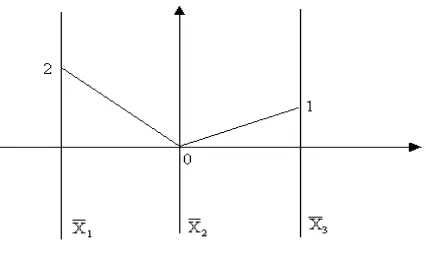
Without loss of generality, we consider the surfaces of revolution generated by the rotation of a curve C in R3 around a line L of equation P(t) = tn, t∈ A ⊆R, n = (n1, n2, n3),

ni ∈R,i= 1,2,3. The curveC is even respect toLand is contained in a plane containing

L.

In order to represent the surface in this system, we need two curvesC₁ and C₂. The first one is the image of the curveCand the second one the image of the curveC, obtained

as the intersection of the surface with appropriate planes. In parallel these planes are the Eickemeyer planes πE₁ and πE₂, respectively. The plane π₁E is generated by the vectors u

andd and the planeπE

2 is generated byuandd, wheredanddare appropriately chosen.

Lemma 4.1 Let n = (n1, n2, n3) , n=0. If n1 = n2 = n3 every Eickemeyer plane contains n and some vector d= (d1, d2, d3), d1 < d2 < d3.

Proof. The planes of the form (d3−d2)x+ (d1−d3)y+ (d2−d1)z = 0 contains the vector nand any vector d= (d1, d2, d3),then we can choose it so thatd1 < d2< d3. QED

Without loss of generality, in what follows we suppose that the vectorn= (n1, n2, n3)

is not parallel to u. Let, for example, n2=n3 ,n2< n3.The following results are valid.

Theorem 4.1 There exists an Eickemeyer’s plane that contains the vectorn= (n1, n2, n3) and a vector d= (d1, d2, d3) , d1 < d2< d3 if and only if n1 < n2.

Proof. If n1< n2 < n3, it´s enough to choosed=n.

Letπ be the Eickemeyer’s plane that contains the vector d. Then:

d1(n2−n3) +d2(n3−n1) +d3(n1−n2) = 0.

Considering a fixed but arbitraryd3 ≥0, it follows that:

d1=

n3−n1

n₃−n₂ d2+

n1−n2

n₃−n₂ d3.

Then we have found a linear relationship betweend1 and d2. In order to ensure that

exists a vector d satisfying the required conditions, it must be:

n₃−n₁ n3−n2

>1;

and then n1 < n2. QED

From this theorem follows only those surface of revolution withn1 < n2 < n3 could

be represented using Eickemeyer’s planes. This motivates the following definition.

Definition 4.1 The 2-flata πa is the 2-dimensional vector subspace spanned by d and

va= (a,1,1), a∈R.

In what follows, we supposea >0.

Remark 4.1 The 2-flats1 are the Eickemeyer’s 2-flats.

Remark 4.2 If a1-flatalies onπathen the pointsπa1,2,πa2,3 (repectivelyπa1,3,πa2,3) defined in Remark 3.1 are coincident. Therefore, the representation of the 1-flata is a single point

in the a-parallel coordinate system.

Theorem 4.2 If n2 < n3 then exists a2-flata, a <1, that contains n.

- If 0< n3, results that

n3(1−a) +n1−n2<0,

and then follows

K = an2−n1

n3(1−a) +n1−n2

>1.

Then it suffices to choose d₂ < Kd₃. So taking into account that

d1=

an3−n1

n3−n2

d2+

n1−an2

n3−n2

d3, (1)

it follows

d2−d1 =d2

1−an3−n1

n3₋n2

−n1−an2

n3₋n2 d3

= n3−n2−an3+n1

n3₋n2 d2−

n1−an2

n3₋n2 d3

= n3(1−a)+n1−n2

n3−n2 d2−

n1₋an2

n3−n2 d3.

(2)

From the last member of Equations (2) we have the following inequality

d₂−d₁ >n3(1−a)+n1−n2

n3₋n2 −

n1−an2

n3₋n2

d₃

> (n3−n2)(1−a)

n3₋n2 d3

= (1−a)d3 >0,

and then it is possible to conclude thatd₁ < d₂ .

- Ifn₃ <0 then we have

−K=− an2−n1

n3(1−a) +n1−n2

>1

So, for anyd2< d3 it is enough to choose

d₁= an3−n1

n3−n2

d₂+n1−an2

n3−n2

d₃,

and then follows thatd1 < d2.

- Ifn3 = 0, we have

d1 =

n1

n2

d2+

an2−n1

−n2

d3.

Asn₁ > n₂ , with n₂<0 results that

n1

n2

<1.

Then

K= an2−n1

n1−n2

<1,

The geometric interpretation of the proof of Theorem 4.2 is as follows.

Consider in the plane two perpendicular axes, and call themd1andd2, andd3 any real number. We can think d₁ = an3₋n1

n3−n2 d2 +

n1₋an2

n3−n2 d3 as a line L in this system coordinate.

The intersection between L and the lined1 =d2 is the point of coordinates: (Kd3, Kd3), where K= an2₋n1

n3(1−a)+n1−n2.

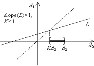
Case 1. If the slope of L is less than one it must be K < 1, in order to exist d2 ∈ (Kd3, d3) that satisfies the given condition (see Figure 2).

Case 2. If the slope of L is greater than 1, it must beK >1. In this case anyd₂ < d₃

satisfies the given requeriment, as can be seen from Figure 3.

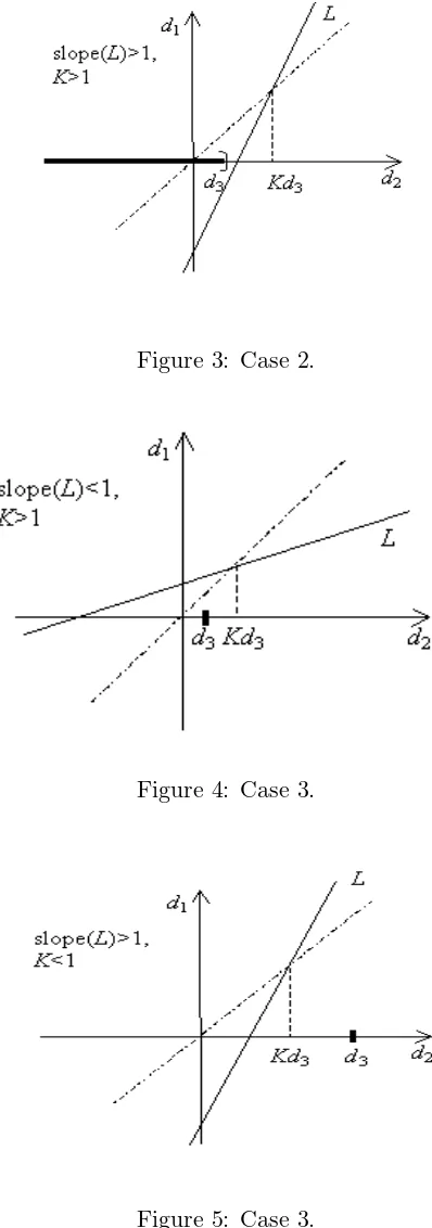
Case 3. Ifa <1 the cases slope ofLgreater than one andK <1 or slope of Lless than one and K >1 are not possible as is shown in Figures 4 and 5.

Ifa >1 the cases mentioned in the last paragraph are possible. Then, choosingd2 < Kd3

for Case 1, the vector d is determined. This shows that Theorem 4.2 gives a necessary but not a sufficient condition, as follows from Example 4.2.

Example 4.2 If a = 2, n = (2,1,3), d = (−2,−1,1) and v2 = (2,1,1) then n is con-tained in the 2-flat2 generated by v2 andd.

Figure 2: Case 1.

Figure 3: Case 2.

Figure 4: Case 3.

Figure 5: Case 3.

Proof: Let a >2. Then

and it results

an3−n1

n₃−n₂ >1.

As (a−1)n2 <(a−1)n3, then

an2−n1

n₃(a−1) +n₂−n₁ <1.

So it suffices to choosed2∈(Kd3, d3). QED

Example 4.3 Letn= (−1,3,5). Then we can choosea= 3 ,d= (−d3−2,−d3−1, d3), so that n is contained in the 2−flat3 generated by v3 y d.

Let πa be the plane generated by d and va and πa be the plane generated byd and

va. The curves C and C are found as the intersection of the surface with the planes πa

and πa, respectively.

According to Section 3 and Remark 4.2 we represent, in the a-parallel coordinate

system, each tangent line to the curveC and C, respectively . These sets, namedC₁ and

C2 represent the curves C andC, respectively. Now we can summarize the procedure as follows.

Step 1. _{Choosed3 >0 and fix any a >1.}

Step 2. _Choosed₂ according to Theorem 4.2.

Step 3. _{Setd1 given by (1).}

Step 4. _{Letd= (d}′

1, d2, d3) such that d′1 > d3.

Step 5. _{Draw, in the a-parallel coordinate system, the curves C and C.}

5

Example of Application

Let us consider the surface of revolution generated by the rotation of the the curve C in

R3 given by: _

       

x =−5t,

y = 5t2, t >0, z = 8t2+t,

around the line of equationP(λ) = (−1,3,5))λ, λ≥0. The curveCis given by equation:         

x = cosα,

y = sinα, α∈[0,2π), z = cosα−2 sinα+ 26.

(4)

Choosing a= 3 we have, according to Theorem 4.2, d = −d₃,₂1d₃, d₃, withd₃ >0 and d =2d3,1₂d3, d3. The curve C belongs to πa, the plane generated by d and va =

(3,1,1) and the curveC belongs toπa, the plane generated by ˜d and va.

The points that represent the curve C in the 3-parallel coordinate system are given

by:

π3₁₂=

d3(1−12t) 2 (6t+ 1) ,

−5t2

(6t+ 1)

, t >0. (5)

For the curveC these points are given by the following expression:

π3₁₂=

d₃6 cosα+1₂sinα

3 cosα+ sinα ,

1 3 cosα+ sinα

, α∈[0,2π). (6)

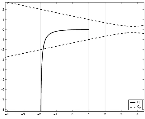
In Figure 6 are shown bothC₁ and C₂, the curves obtained when drawing the points given by equations (5) and (6), withd3= 2.

−4 −3 −2 −1 0 1 2 3 4

−8 −7 −6 −5 −4 −3 −2 −1 0 1 2 C 1 C 2

Figure 6: Representation of a surface of revolution in the 3-parallel coordinate system.

6

Conclusions

that generalizes the work of Hung and Inselberg for representing surfaces of revolution.

To do this, it was necessary to define our so called a-parallel coordinate system. This new system allows for the representation of developable, ruled and revolution surfaces in 3D.

Although the methodology is restricted to 3D surfaces, we are are working on its extension to N-dimensional hypersurfaces of revolution. In this case, all the applications known so

far for ruled and developable surfaces could be extended to a wider class of hypersurfaces.

References

[1] Chatterjee, A. and A. InselbergVisualizing multi-dimensional polytopes and topologies

for tolerances. Research Report RC 20133 (89022), IBM Reserach Division, Yorktown Heights, New York, 1995.

[2] Inselberg, A. and B. Dimsdale. Multidimensional lines I: representation. SIAM

Jour-nal of Applied Mathematics, Volume 54, Number 2, pages 559-577, 1994.

[3] Inselberg A., J. Hassett and A. Chatterjee.Visualization of Multi-dimensional

Geom-etry and Application to Multi-variate Problems. SIGGRAPH’95 Course Notes, Course No. 27, 1995.

[4] Inselberg, A and C.K. Hung. A new representation of hypersurfaces in terms of

tan-gent hyperplanes. Proc. of SIAM Conference on Geometric Design, 11, 1991.