Reusing Optimal TSP Solutions for
Locally Modified Input Instances
⋆(Extended Abstract)
Hans-Joachim B¨ockenhauer1, Luca Forlizzi2, Juraj Hromkoviˇc1, Joachim Kneis3⋆⋆, Joachim Kupke1, Guido Proietti2,4, and Peter Widmayer1
1
Department of Computer Science, ETH Zurich, Switzerland,
{hjb,juraj.hromkovic,jkupke,widmayer}@inf.ethz.ch
2
Department of Computer Science, Universit`a di L’Aquila, Italy,
{forlizzi,proietti}@di.univaq.it
3
Department of Computer Science, RWTH Aachen University, Germany,
4
Istituto di Analisi dei Sistemi ed Informatica “A. Ruberti”, CNR, Roma, Italy
Abstract. Given an instance of an optimization problem together with an optimal solution, we consider the scenario in which this instance is modified locally. In graph problems, e. g., a singular edge might be removed or added, or an edge weight might be varied, etc. For a problem Uand such a local modification operation, letlm-U
(local-modification-U) denote the resulting problem. The question is whether it is possible to exploit the additional knowledge of an optimal solution to the original instance or not, i. e., whetherlm-U is computationally more tractable thanU. Here, we give non-trivial examples both of problems where this is and problems where this is not the case. Our main results are these: 1. The local modification to change the cost of a singular edge turns the traveling salesperson problem (TSP) into a problemlm-TSP
which is as hard as TSPitself, i. e., unless P = N P, there is no polynomial-timep(n)-approximation algorithm forlm-TSPfor any
polynomialp. Moreover,lm-TSPwhere inputs must satisfy the β-triangle inequality (lm-∆β-TSP) remains NP-hard for allβ > 1
2. 2. Forlm-∆-TSP(i. e., metriclm-TSP), an efficient
1.4-approxima-tion algorithm is presented. In other words, the addi1.4-approxima-tional informa-tion enables us to do better than if we simply used Christofides’ algorithm for the modified input.
3. Similarly, for all 1< β <3.34899, we achieve a better approxima-tion ratio forlm-∆β-TSPthan for∆β-TSP.
4. Metric TSP with deadlines (time windows), if a single deadline or the cost of a single edge is modified, exhibits the same lower bounds on the approximability in these local-modification versions as those currently known for the original problem.
⋆This work was partially supported by SNF grant200021-109252/1, by the research
project GRID.IT, funded by the Italian Ministry of Education, University and Research, and by the COST 293 (GRAAL) project funded by the European Union.
1 Introduction
Traditionally, optimization theory has been concerned with the task of finding good feasible solutions to (practically relevant) input instances, little or nothing about which is known in advance. Many applications, however, demand good, sometimes optimal, solutions to a limited set of input instances which reflect a supposedly-constant environment (imagine, e. g., an existing railway system or communications network). When this environment does change, maybe only slightly and maybe only locally, do we have no choice but to recompute some good feasible solution, effectively forgetting about the old one?
Here, we will analyzelocal modifications only. In a graph problem, for ex-ample, the cost of a single edge might change, an edge might be removed or added, or some other local parameter might be adjusted. Results related to this work pertain to the question by how much a given instance of an optimization problem may be varied if it is desired that optimal solutions to the original in-stance retain their optimality [12, 17, 18, 20, 21]. In contrast with this so-called “postoptimality analysis,” our approach here is to ask, if we cannot avoid to lose the optimality of a given solution when an instance is varied arbitrarily, what can we do torestore the quality of a solution, maybe in an approximative sense?
Surely, for some problems, knowing an optimal solution to the original in-stance trivially makes their local-modification variants easy to solve because the given optimal solution is itself a very good solution to the modified instance. For example, adding an edge in the instance of a coloring problem will increase the cost of an optimal solution by at most the amount of one – an excellent approximation, but certainly not the object of our interest.
Our goal is to present non-trivial examples of problems, some where the knowledge of an optimal solution to an instance close to the input is helpful and some where it is not. To this end, we will studyTSP, its restricted versions,
and its generalizations such asTSPwith deadlines (a special case of TSPwith
time windows).
Let∆-TSPdenote metric TSP, and, for allβ ≥1
2, let∆β-TSPdenote the special case of TSP where all instances satisfy theβ-triangle inequality
c({x, z})≤β· c({x, y}) +c({y, z}) for all verticesx,y, and z. If 1
2 ≤β <1, we call this thestrengthened triangle inequality; and ifβ >1, we call it therelaxed triangle inequality.
For an optimization problemU, we denote our local-modification variant of
U bylm-U. For the aforementionedTSP-based problems, we regard it as a local
modification to change the cost of exactly one edge. For TSP with deadlines,
we also regard it as a local modification to shift one deadline by the amount of at least one time unit.
Our main results are as follows:
(i) It is well-known that TSP is not approximable in polynomial time with
holds forlm-TSP, too. Thus, in terms of a worst-case analysis, lm-TSP
is as hard asTSP, and we do not have anything to gain from knowing an
optimal solution to a close problem instance. By parameterizingTSPwith
respect to the β-triangle inequality [1, 2, 3, 4, 5] and by introducing the concept of stability of approximation [15, 5], it was shown thatTSPis not
as hard as it may look like in the light of worst-case analyses. For anyβ > 12, we have a constant polynomial-time approximation ratio, depending onβ
only. B¨ockenhauer and Seibert [8] proved that ∆β-TSP is APX-hard for every β > 12 (note that for β = 1
2, the problem becomes trivially solvable in polynomial time). Here, we prove thatlm-∆β-TSPis NP-hard for every
β > 12. This implies in particular that lm-∆-TSP, too, is NP-hard. We
conjecture that this problem is also APX-hard, which, so far, we have been unable to prove and thus leave as an open research problem.
(ii) For many years, Christofides’ algorithm [9] with its approximation ratio of 1.5 has been the best known approximation algorithm for attacking
∆-TSP. It remains a grand challenge to improve on Christofides’ algorithm.
We will show that, intriguingly enough,lm-∆-TSPadmits an efficient 1.
4-approximation algorithm. This result can be generalized tolm-∆β-TSP,
and the resulting approximation guarantee beats all previously-known ap-proximation algorithms for∆β-TSPfor all 1< β <3.34899, which includes the practically most relevantTSPinstances.
(iii) TSPwith time windows is one of the fundamental problems in operations
research [10]. Usually, only heuristic algorithms are used to attack it al-though the question how hard it is w. r. t. approximability has only been resolved in [6, 7], where even anΩ(n) lower bound on the polynomial-time approximability of∆-TSPwith time windows was shown, in contrast to the
constant approximability of∆-TSP. This lower bound already holds for the
special case of this problem where all time windows are immediately open, a special case of the problem which we will callTSPwith deadlines, or∆ -DlTSPfor short. Here, we consider local-modification versions of∆-TSP
with deadlines. We show that already if we only allow a single deadline to be changed, and only by an amount of one time unit, the resulting problem,
lm-∆-DlTSP, has the same lower bound of Ω(n) on the approximation
ratio as∆-DlTSP. Let us underscore the importance of this negative
re-sult: Not only does TSP with deadlines remain an intractable problem in itslmversion, but the extra knowledge of an optimal solution to a related
instance does not even help a single bit. Likewise, we will establish the lower bound of (2−ε), for anyε >0, for lm-∆-DlTSPwith a constant number
of deadlines, the same as is known for∆-DlTSPwith a constant number
of deadlines [6, 7]. These results can also be obtained if, again, we modify the cost of an edge rather than a deadline.
the hardness of local-modification optimization problems in order to develop approaches to handle situations where multiple (and, potentially, dynamically determined) local modifications may arise.
The paper is subdivided into two main sections. In Section 2, we will analyze TSP with local modifications and present hardness results as well as approxi-mation algorithms for the metric and near-metric case. Section 3 is devoted to inapproximability results for the local-modification version of TSP with dead-lines.
2 Results for TSP
In this section, we will analyze the local-modification version of TSP. In Subsec-tion 2.1, we will present our hardness results. In SubsecSubsec-tion 2.2, we will present a 1.4-approximation algorithm for the local-modification metric TSP, and Sub-section 2.3 is devoted to approximability results for the case of the relaxed triangle inequality.
We start off with a formal definition of TSP and its local-modification
variants.
Definition 1.Let G= (V, E, c) be a weighted complete graph, and let β ≥ 1 2
be a real value. We say that Gobeys the ∆β-inequality iff for all vertices x,y,
z∈V, we have
c({x, z})≤β· c({x, y}) +c({y, z}) . (∆β)
By TSP, we denote the following optimization problem. For a given weighted
complete graph G= (V, E, c), find a minimum cost Hamiltonian cycle, i. e., a tour on all vertices of cost
OTG:= min
( X
e∈C′
c(e)
(V, C′)is a Hamiltonian cycle
)
.
Restricting, for some value of β, the set of admissible input instances to those which obey the ∆β-inequality yields the problem ∆β-TSP. Besides,
de-fine∆-TSP:=∆1-TSP.
Definition 2.LetU ∈ {TSP, ∆-TSP, ∆β-TSP}. The problemlm-U is defined
as follows.
Input:
– two complete weighted graphsGO= (V, E, cO),GN = (V, E, cN)such thatGO
andGN are both admissible inputs forU and such that cO andcN coincide,
except for one edge;
– a Hamiltonian cycle(V, C)such that P
e∈C
cO(e) =OTGO.
Problem: Find a Hamiltonian cycle(V, C)that minimizes P
e∈C
2.1 Hardness Results
Before presenting approximation algorithms forlm-∆-TSP, we start by proving
some hardness results.
First, we will show thatlm-TSPis as hard to approximate as “normal” (i. e.,
unaltered) TSP.
Theorem 1.There is no polynomial-time p(n)-approximation algorithm for
lm-TSP for any polynomial p(unless P =N P).
Proof idea.We will give a reduction from the Hamiltonian cycle problem (HC): Given an undirected, unweighted graphG, decide whetherGcontains a Hamil-tonian cycle or not. Let G = (V, E) be an input instance for HC where
V ={v1, . . . , vn}.
In order to construct an input instance (GO, GN, C) forlm-TSP, we employ a graph construction due to Papadimitriou and Steiglitz [19], who used the same construction in order to give examples of TSP instances which are hard for local search strategies: For each vertexvi, we construct a so-called diamond graphDi as shown in Figure 1 (a). These diamonds are connected as shown in Figure 1 (b).
The edge costs inGO are set as follows. Let M :=n·2n+ 1. All diamond edges shown in Figure 1 (a) and the connections fromEi toWi+1and fromEn to W1 as shown in Figure 1 (b) are assigned a cost of 1 each. Edges{Ni, Sj} are assigned a cost of 1 whenever {vi, vj} ∈ E and a cost ofM otherwise. All other edges receive a cost ofM each. InGN, the cost of the edge{En, W1} is changed from 1 toM. The given optimal Hamiltonian cycleCis the one shown in Figure 1 (b). This optimal solution forGO has a cost of 8n.
It is easy to see that if there is a Hamiltonian cycleH′inG, a corresponding
Hamiltonian cycleH inGcan traverse all diamonds fromNi viaWi via Ei to
Si. Hence,cN(H) = 8n. All Hamiltonian cycles inGN that do not correspond (in this way) to Hamiltonian cycles in Gcost at least M + 8n−1. Thus, the approximation ratio of any non-optimal solution is at least as bad as 1 + 2n−3. For a more detailed description of diamond graph constructions, also see, for
example, [16].
Si
Ei
Wi
Ni
(a)
S1
E1
W1
N1
S2
E2
W2
N2
Sn
En
Wn
Nn
[image:5.612.136.478.514.603.2](b)
Now, we will show thatlm-∆-TSPremains a hard problem for any β >1 2. Theorem 2.lm-∆β-TSPis NP-hard for any β > 1
2.
Proof.We will use a reduction from the restricted Hamiltonian cycle problem (RHC). The objective in RHC is, given an unweighted, undirected graphGand a Hamiltonian pathP inGwhich cannot be trivially extended to a Hamiltonian cycle by joining its end-points, to decide whether a Hamiltonian cycle in G
exists. This problem is well-known to be NP-complete (see, for example, [16]). The reduction uses an idea analogous to the standard reduction from the Hamiltonian cycle problem to TSP: Let (G, P) be an instance of RHC where
G= (V, E),V ={v1, . . . , vn}, andP = (v1, . . . , vn). From this, we construct an instance (GO, GN, C) oflm-∆β-TSPas follows: LetGO= (V,E, c˜ O) andGN = (V,E, c˜ N) where (V,E˜) is a complete graph,cO(e) = 1 for alle∈E∪ {{vn, v1}} andcO(e) = 2β otherwise, andcN({vn, v1}) = 2β. LetC = (v1, v2, . . . , vn, v1). Clearly, this reduction can be done in polynomial time, and it is easy to see that there is a Hamiltonian cycle inGiff there is a Hamiltonian cycle of costn
in GN.
2.2 The Metric Case
In what follows, we will show thatlm-∆-TSPadmits a 7
5-approximation, which beats the na¨ıve approach of using Christofides’ algorithm (which would yield a
3
2-approximation), whereby the input cycle (V, C) would be ignored altogether. Theorem 3.There is a1.4-approximation algorithm forlm-∆-TSP.
In order to prove Theorem 3, we will need the following few lemmas. Our crucial observation is that in a metric graph, all of the neighboring edges of short edges can only be modified by small amounts.
Lemma 1.Let G1= (V, E, c1) andG2= (V, E, c2)be metric graphs such that
c1 and c2 coincide, except for one edgee∈E. Then, every edge adjacent toe
has a cost of at least 12|c1(e)−c2(e)|.
Proof.We set {a, a′} := {c
1(e), c2(e)} such that a′ > a and δ := a′−a. Let
f ∈E be any edge adjacent toe, and for any suchf, letf′∈Ebe the one edge that is adjacent to botheandf. Then, by the triangle inequality, we have:
a′≤c(f) +c(f′) c(f′)≤c(f) +a
and hencea′−a≤2c(f).
We will have to distinguish two cases. Either, an edge becomes more expen-sive, or it becomes less expensive. In either case, our strategy is to compare the input solution (to the old problem instance) with an approximate solution (to the new problem instance).
Lemma 2.Let (GO, GN, C) be an admissible input forlm-∆-TSP such that
δ:=cO(e)−cN(e)>0for the edgee. If OTδGN ≤ 2 5, it is a
7
5-approximation to
output the feasible solution C:=C forlm-∆-TSP.
Proof.
cN(C)
OTGN
≤ cO(C)
OTGN
= OTGO
OTGN
≤OTGN +δ
OTGN
= 1 + δ
OTGN
≤1 + 2 5 =
7 5
Lemma 3.Let (GO, GN, C) be an admissible input forlm-∆-TSP such that
δ:=cO(e)−cN(e)>0 for the edgee. If OTδGN ≥25, there is a 7
5-approximation
forlm-∆-TSP.
Proof.We may assume that optimal TSP tours inGN use the edgee. For if they did not, Cwould already constitute an optimal solution. Fix one such optimal tour COP T in GN. InCOP T,eis adjacent to two edgesf andf′. Letv be the vertex incident with f, but not with e, and let v′ be the vertex incident with
f′, but not withe. ByP, denote the path fromv tov′ in COP T that doesnot involvee.
Consider the following algorithm: For every pair ˜f, ˜f′of disjoint edges, both of which are adjacent to e, compute an approximate solution to the TSP path problem on the subgraph of GN induced by the vertex setV \e(i. e., without
two vertices) with start vertex ˜v and end vertex ˜v′ where {˜v} = ˜f \e and {˜v′}= ˜f′\e. It is known [13, 14] that this can be done with an approximation guarantee of 53. Each of these paths is augmented by ˜f,e, and ˜f′ so as to yield a TSP tour. The algorithm concludes by outputting the least expensive of all of these tours.
Note that sinceall pairs ˜f, ˜f′ are taken into account, one of the considered
tours uses exactly those edges ˜f =f, ˜f′=f′ thatC
OP T uses. This is why the algorithm outputs a tour of cost at most
c(f) +c(f′) +cN(e) + 5
3c(P) = OTGN −c(P)
+5
3c(P) =OTGN +
2 3c(P) (wherec is short-hand notation forcN wherevercO andcN coincide) and thus achieves an approximation guarantee of
1 + 2 3 ·
c(P)
OTGN
.
Since by Lemma 1, min{c(f), c(f′)} ≥ δ
2fori∈ {1,2}, we haveOTGN−c(P)≥δ
and hence:
c(P)
OTGN
≤1− δ
OTGN ≤ 3
5 .
Corollary 1.There is a 75-approximation algorithm for the subproblem of
lm-∆-TSPwhere edges may only become less expensive.
Proof.Compute, as laid out in Lemma 3, an approximate solution tolm-∆-TSP
and compare it with the input solution C. Output the less expensive of the two solutions. Depending on whether the value of δ
OTGN (where δ:=cO(e)−
cN(e)>0) is less or greater than 25 (which we cannot necessarily tell), one of the considered two feasible solutions is a 7
5-approximation.
We will now turn to the case where an edge becomes more expensive. We can state a lemma akin to Lemma 2, but notice that by reusing a formerly optimal solution, we incur a certain extra cost.
Lemma 4.Let (GO, GN, C) be an admissible input forlm-∆-TSP such that
δ:=cN(e)−cO(e)>0for the edgee. If OTδGN ≤ 2 5, it is a
7
5-approximation to
output the feasible solution C:=C forlm-∆-TSP.
Proof.
cN(C)
OTGN
≤ cO(C) +δ
OTGN
= OTGO+δ
OTGN
≤OTGN +δ
OTGN
= 1 + δ
OTGN
≤1 + 2 5 =
7 5
When computing an approximate solution, things become slightly different from what they used to be like in Lemma 3: We may assume thateused to be a part ofC and that a new solution should no longer use it. Instead, it will use two edgesf andf′ such thatf andf′ are non-disjoint and both incident with the same vertex ofe. This pair may be chosen at either end-point ofe, a choice which is completelyarbitrary.
We conjecture that, if an improvement of the approximation guarantee is possible, this is precisely the point where to start at.
Lemma 5.Let (GO, GN, C) be an admissible input forlm-∆-TSP such that
δ:=cN(e)−cO(e)>0 for the edgee. If OTδ
GN ≥ 2
5, there is a 7
5-approximation
forlm-∆-TSP.
Proof.We may assume that optimal TSP tours in GN do not use the edge e. For if they did,C would already constitute an optimal solution. Fix one such optimal tourCOP T, and fix one vertexwincident withe. InCOP T,wis incident with two edges f andf′. Let v be the vertex incident withf, but not with e, and letv′ be the vertex incident withf′, but not withe. ByP, denote the path fromv tov′ in COP T that doesnot involvew.
Consider the following algorithm: For every pair ˜f, ˜f′ of edges incident with
with an approximation guarantee of 53. Each of these paths is augmented by ˜f
and ˜f′ so as to yield a TSP tour. The algorithm concludes by outputting the least expensive of all of these tours.
Note that sinceall pairs ˜f, ˜f′ are taken into account, one of the considered tours uses exactly those edges ˜f =f, ˜f′=f′ thatC
OP T uses. This is why the algorithm outputs a tour of cost at most
c(f) +c(f′) +5
3c(P) = OTGN −c(P)
+5
3c(P) =OTGN+
2
3c(P) ,
just as in the proof of Lemma 3.
Using the same arguments as in the proof of Corollary 1, the preceding lemma yields the following corollary.
Corollary 2.There is a 75-approximation algorithm for the subproblem of
lm-∆-TSPwhere edges may only become more expensive.
2.3 The Near-Metric Case
The algorithm outlined in Lemma 3 can be generalized to graphs which are not necessarily metric, but only near-metric, i. e., where the metricity constraint is relaxed by a factor of β. Since it will pay off later, let us pay extra attention to the fact that input instances for all the problems from Definition 2 contain two distinct graphs, potentially obeying relaxed triangle inequalities according to different values ofβ.
Notice that the parameter β need not be greater for the graph with the costlier edge. Under some circumstances, it might even decrease when we mod-ify the cost of a single edge. In the following generalization of Lemma 1, the convention is therefore thatc1is the cost function of the less expensive graph,c2 that of the more expensive one, and bothciobey the∆βi-inequality,i∈ {1,2}.
Lemma 6.LetG1= (V, E, c1)andG2= (V, E, c2)be graphs such thatciobeys
the ∆βi-inequality for i∈ {1,2} and some values β1, β2 ≥1 and such that c1
and c2 coincide, except for one edge e ∈E. By convention, let c1(e) ≤c2(e).
Then, every edge adjacent to ehas a cost of at least c2(e)−β1β2c1(e)
β1β2+β2 .
Proof.Analogous to Lemma 1.
Note that for relatively small changes, the valuec2(e)−β1β2c1(e) may well be non-positive, rendering Lemma 6 trivial in such a case.
Algorithm 1
Input: An instance (GO, GN, C) of lm-∆β-TSP where GO = (V, E, cO) and GN =
(V, E, cN).
1. Lete∈Ebe the edge wherecO(e)6=cN(e).
LetEbe the set of all unordered pairs{f, f′} ⊆Ewheref6=f′are edges adjacent toesuch that ifcO(e)< cN(e):f∩f′∩eis a singleton; and
ifcO(e)> cN(e):f∩f′=∅.
2. For all {f, f′} ∈ E, compute a Hamiltonian path between the two vertices from (f∪f′)\eon the graphG\(e∩(f∪f′)), using the PMCA path variant by Forlizzi et al. [11]. Augment this path by edgesf, f′, and, if c
O(e) > cN(e), edge e to
obtain the cycleC{f,f′}.
3. LetCbe the least expensive of the cycles in the set{C} ∪ {C{f,f′}| {f, f′} ∈ E}.
Output: The Hamiltonian cycleC.
Lemma 7.Algorithm 1 achieves an approximation guarantee of
βLβH·
15β2L + 5βL−6 10β2
L + 3βLβH+ 3βH−6
(1)
for input graph pairs(GO, GN)such thatGO obeys the∆βO-inequality andGN
obeys the∆βN-inequality and whereβL:= min{βO, βN}andβH:= max{βO, βN}.
Proof.Adhering to the convention of Lemma 6, set {c1, c2} = {cO, cN} such that c1(e)≤c2(e) for all edges e∈ E. In other words, we havec2 =cN if an edge becomes more expensive andc1=cN otherwise.
We may assume that optimal TSP tours inGN = (V, E, cN) use the edgee iffcN =c1; otherwise,C is an optimal solution, and we are done. Fix one such optimal tourCOP T in GN, and let{f, f′} ∈ E be such thatCOP T uses bothf and f′. By P, denote the path that results from COP T by removing edges f,
f′, and, potentially,e. Set
α:= C(P)
OTGN
and let, for brevity, ϑ:=βLβH·
15β2
L + 5βL−6 10β2
L + 3βLβH+ 3βH−6 denote the approximation guarantee claimed in (1). In terms ofα, Algorithm 1 always achieves an approximation guarantee of
1−α
| {z }
edgesf,f′, (potentially)eare chosen optimally
+ 5
3β 2 Lα
| {z }
P will be approximated
,
even if we did not haveCat our disposal. (Note that the strategy to approximate
α > 5ϑ−1
3β2L −1
, (2)
we are done. Let use therefore assume that (2) holds. By Lemma 6, we have
min{c(f), c(f′)} ≥ c2(e)−β1β2c1(e)
β1β2+β2
≥c2(e)−βLβHc1(e)
βLβH+βH and hence
1−α≥ 2·(c2(e)−βLβHc1(e))
OTGN ·(βLβH+βH)
.
Putting this together with (2), we know that
ϑ−1 5 3βL2−1
≤1−2·(c2(e)−βLβHc1(e))
OTGN ·(βLβH+βH)
,
which yields
c2(e)−βLβHc1(e)
OTGN
≤ βLβH+βH
2 −
(ϑ−1)·(βLβH+βH) 10
3βL2−2
.
By adding (βLβH−1) c1(e)
OTGN to both sides, we are given:
c2(e)−c1(e)
OTGN
≤ βLβH+βH
2 −
(ϑ−1)·(βLβH+βH) 10
3βL2−2
+ (βLβH−1)·
c1(e)
OTGN
| {z }
≤1 and thus, substituting the value (1) forϑ,
c2(e)−c1(e)
OTGN
≤3 2βLβH+
1
2βH−1−
(ϑ−1)·(βLβH+βH) 10
3βL2−2
= 3 2βLβH+
1
2βH−1− (βLβH·
15β2
L+5βL−6 10β2
L+3βLβH+3βH−6−1)(βLβH+βH) 10
3βL2−2
(tedious calculations) =· · ·=βLβH·
15βL2+ 5βL−6 10β2
L + 3βLβH+ 3βH−6
−1 =ϑ−1 .
Since, by the same reasoning as that of Lemmas 2 and 4, reusing the input optimal solutionCinflicts a deviation from the new optimum by at mostc2(e)−
c1(e)≤(ϑ−1)·OTGN, Algorithm 1 is aϑ-approximation algorithm.
Hence, whenever theβ values ofGO andGN coincide, we have Theorem 4.
Theorem 4.There is a (polynomial-time) β2·15β
2+ 5β−6
13β2+ 3β−6-approximation
4β
3 2β
2
β2+β
Algorithm 1
β∗
Cor. 3
1 1.5 2 2.5 3 3.5
1 3 5 7 9 11 13
Parameterβ
[image:12.612.139.468.88.265.2]Approximation guarantee
Fig. 2. Approximation guarantees of various algorithms, depending onβ
Interestingly, Algorithm 1 achieves a better approximation guarantee not just than PMCA [5], but also than Bender’s and Chekuri’s 4β-approximation algorithm [3] for the most practically relevant values ofβ. The turning point is about atβ∗≈3.34899. More to the point, Andreae’s (β2+β)-approximation [1], which performs better than 4β only when β <3, always performs worse than Algorithm 1 in the interval β ∈ (1, β∗). These observations are illustrated in
Figure 2.
Another practical special case is that whereβL = 1, i. e., where we start with a metric graph, but changing the cost of an edge will violate the∆-inequality.
Corollary 3.lm-∆β-TSP, restricted to those inputs whereGO is metric,
ad-mits a 2+37ββ-approximation.
3 Deadline TSP
In this section, we will analyze the approximability of local-modification variants of TSPwith deadlines. To begin with, let us define this problem formally.
Definition 3.Let G = (V, E) be a complete graph weighted by c: E → ◆+.
We call (s, D, d) a deadline set forG ifs∈V, D⊆V \ {s} and d:D →◆+.
A vertex v ∈ D is called deadline vertex. A path (v0, v1, . . . , vn) satisfies the deadlinesiffs=v0 and, for allvi∈D, we havePij=1c({vj−1, vj})≤d(vi).
A cycle(v0, v1, . . . , vn, v0) satisfies the deadlines iff it contains a path (v0,
v1,. . .,vn)satisfying the deadlines.
Definition 4.The problem∆β-DlTSPis defined as follows: For a given
-inequality, deadlines (s, D, d) for G, and a Hamiltonian cycle satisfying the deadlines1, find a minimum-weight Hamiltonian cycle satisfying all deadlines.
If |D| is a constant k, the resulting subproblem is k-∆β-DlTSP. We set
∆-DlTSP:=∆1-DlTSPandk-∆-DlTSP:=k-∆1-DlTSP for allk.
In the case ofTSPwith deadlines, we will regard it as a local modification
to change a single deadline although thelmoperation from the previous section
would let us obtain exactly the same results. The connection between these two
lmoperations will be presented in detail in the journal version of this paper.
Definition 5.The optimization problem lm-DlTSP is defined as:
Input: A complete weighted graph G= (V, E, c), deadlines O = (s, D, dO) for
Gwith a minimal Hamiltonian cycle satisfying the deadlinesO, new deadlines
N = (s, D, dN)such thatdO anddN differ in exactly one vertex, and a
Hamil-tonian cycle satisfyingN.
Problem: Find a minimum-cost Hamiltonian cycle satisfyingN.
By lm-k-DlTSP, lm-∆-DlTSP, lm-k-∆-DlTSP, lm-∆β-DlTSP,
lm-k-∆β-DlTSP, we denote the canonical special cases of lm-DlTSP.
For our proofs, we will need some reductions from the following problem, which can easily be shown to be hard analogously to the proof of the NP-hardness of therestricted Hamiltonian cycle problem,as presented, e.g., in [16]. Definition 6.For a given graph G= (V, E),s, t ∈ V and a given Hamilto-nian path P from s tot, the problem RHP is to decide whetherG contains a
Hamiltonian path starting ins, but ending in some vertex v6=t.
3.1 Bounded Number of Deadline Vertices
We start with the case where only few deadline vertices occur. Note thatk-∆ -DlTSPcan be approximated within a ratio of 2.5 [6, 7]. Furthermore, a lower
bound of 2−εon the approximability, for everyε >0, can be proved [6, 7]. We will show that this lower bound also holds forlm-k-∆-DlTSP.
Theorem 5.Letε >0. There is no polynomial-time(2−ε)-approximation al-gorithm for the subproblem of lm-k-∆-DlTSPwhere one deadline is increased
by ξtime units,ξ≥1, unlessP =N P.
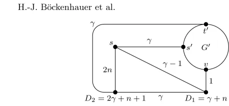
Proof.By means of a reduction, we will show that such an approximation algo-rithm could be used to solveRHP. Letε >0.
Let (G′, P) be an input instance forRHPwhereG′= (V′, E′),|V′|=n+ 1,
s′, t′ ∈V′, andP is a Hamiltonian path from s′ to t′. Pick a γ > 5n2+3ε (which implies 24γγ+3+nn−+11 >2−ε).
1
γ
2n γ−1
1
γ γ
s
D2= 2γ+n+ 1 D1=γ+n
G′ s′
[image:14.612.149.378.74.180.2]v t′
Fig. 3. Increasing a deadline. All verticesv′∈V′\ {s′, t′}are connected likev.
We construct a complete weighted graphG= (V, E, c) as part of an input for lm-k-∆-DlTSPas shown in Figure 3: We set V :=V′∪{˙ s, D
1, D2}, and, for any edge e between two vertices v1, v2 ∈ V′, let c(e) = 1 if e ∈ E′ and
c(e) = 2 otherwise. All edges depicted in Figure 3 have the indicated costs while non-depicted edges obtain maximal possible costs.
For these deadlines, one optimal solutionCis the cycles, D1, D2, t′, . . . , s′, s, which uses the Hamiltonian pathP froms′ tot′ inG′. It costs exactlyγ−1 + γ+γ+n+γ= 4γ+n−1. All other feasible solutions visit some vertices inV′
betweensandD1, but cost at least the amount of 1 more.
Now, we increase d(D1) by ξ. If G′ contains a Hamiltonian path P from
s′ to some vertexv6=t′, a new optimal solution iss, P, D1, D2, s, and it costs
γ+n+ 1 +γ+ 2n= 2γ+ 3n+ 1. IfG′ does not contain such a path, it is not possible to visit all vertices inV′before reachingD1andD2. Asc({t′, D1})≥2, we cannot follow the given Hamiltonian pathP because this would violate the deadline d(D2). Similar arguments hold for every other possibility. Hence, C remains an optimal solution in this case. Thus, we could use any approximation algorithm with an approximation guarantee better than
4γ+n−1
2γ+ 3n+ 1 >2−ε
to solveRHP. This is why approximating this subproblem oflm-k-∆-DlTSP
within 2−εis NP-hard for allk≥2.
Theorem 6.Letε >0. There is no polynomial-time(2−ε)-approximation al-gorithm for the subproblem of lm-k-∆-DlTSPwhere one deadline is decreased
by ξtime units,ξ≥1, unlessP =N P.
Proof.Let ε > 0. Like in the preceding proof, we will use a reduction from
RHP.
Let (G′, P) be an input instance forRHPwhereG′= (V′, E′),|V′|=n+ 1,
s′, t′ ∈V′, andP is a Hamiltonian path froms′ to t′. Pick some γ such that
4γ
2γ+8n >2−ε.
We construct a complete weighted graphG= (V, E, c) as part of an input forlm-k-∆-DlTSPas shown in Figure 4: We setV :=V′∪{˙ s, D
s
D1= 2n
D2= 2n
D3=γ+ 5n
D4= 2γ+ 5n
n
n n
γ−1
γ γ+ 1
γ
2n
3n
G′ v t′
s′
[image:15.612.173.436.95.166.2]γ
Fig. 4. Decreasing a deadline. All verticesv′∈V′\ {s′, t′}are connected likev.
c(e) = 2 otherwise. All edges depicted in Figure 4 have the indicated costs while non-depicted edges obtain maximal possible costs.
The initial deadlines are depicted in Figure 4. In this setting, an optimal solution is the cycle s, D2, D1, t′, . . . , s′, D3, D4, s, which contains the Hamilto-nian path froms′ tot′. This path costs 2n+γ−1 on its way to G′, spendsn
on the path fromt′ to s′, and reachessat time 2γ+ 8n−1.
Now, we decrease the deadlined(D1) byξ, whereby the old optimal solution becomes infeasible. Any new solution must visitD1beforeD2. If we try to reuse the Hamiltonian path fromt′ tos′, we have to spend 2n+γ+ 1 on the way to
t′. Therefore, we cannot reachD3if we follow the complete Hamiltonian path. Furthermore, we cannot visit any vertex v ∈ V′ between visiting D3 and D4 because D3 is not reached before 4n+γ, going back toV′ would cost another 2n, and the cheapest path fromV′ to D4 costs more than γ. This is why any solution using a Hamiltonian path betweens′andt′violates one of the deadlines
d(D3),d(D4).
IfG′ contains a Hamiltonian pathP froms′ to somev6=t′, the new optimal solution contains this path in reverse on its way toD3. The paths, D1, D2, P, D3 visits all vertices inV′betweenvands′and reachesD
3at timeγ+5n. Therefore, this new optimal solution costs 2γ+ 8n.
IfG′ does not contain such a Hamiltonian path, the optimal solution cannot
visit all vertices in V′ before reaching D
3 or even D4, and consequently, it is more expensive than 4γ. Thus, we could use an approximation algorithm with an approximation guarantee better than
4γ
2γ+ 8n >2−ε
to solve RHP. Hence, approximating this subproblem of lm-k-∆-DlTSP
within 2−εis NP-hard.
3.2 Unbounded Number of Deadline Vertices
When the number of deadline vertices is unbounded, we can show a linear lower bound on the approximability oflm-∆-DlTSP. Our reduction from RHP
instance. A second construction inflates this advantage. Tours which start at timeX, different from those that start between timesX+gandX+ζg, may spend some extra time to visit a group of vertices which, unless visited early, will cause belated tours to runktimes zigzag across a huge distanceγ.
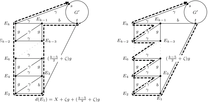
The following lemma describes the construction in detail. See Figure 5 for an overview.
Lemma 8.LetX, g, k, γ, ζ ∈◆such thatkis even,ζ≥1andγ≥g. LetG′ = (V′, E′)be a graph with deadline set(s, D′, d′)such that any Hamiltonian path inG′ respecting the deadlines ends in the same vertext. Then, we can construct a complete graph G⊃G′ and deadlines (s, D, d)such that D ⊃D′,d|D′ =d′
and any path that reaches t in timeX can be extended to a Hamiltonian cycle which costs at most
X+ (k+ 2ζ−4)g+ 2γ ,
while any path that reachestafterX+g, but beforeX+ζgcan only be extended to a Hamiltonian cycle which costs at least
X+
k−3 2 +ζ
g+kγ .
Proof.We constructG= (V, E) with V =V′∪ {E
1, . . . Ek} and edge costs as depicted in Figure 5, whereb:=g(ζ−12). To all other edges, we assign maximal possible costs. Note that the edge {t, E1} costs exactly the same as the path
Ek−1, Ek−3, . . . , E1. We set the deadlines
s
t G′
E3
Ek−3
Ek−1
E2
E4
E6
Ek−2
Ek
(k−5 2 +ζ)g
b b g g g g g γ γ γ γ γ γ γ γ γ E1 s t G′ E3
Ek−3
Ek−1
E2
E4
E6
Ek−2
Ek
(k−5 2 +ζ)g
b b g g g g g γ γ γ γ γ γ γ γ γ
d(E1) =X+ζg+ (
[image:16.612.140.476.421.586.2]k−5 2 +ζ)g
Fig. 5.The zigzag construction for the proof of Lemma 8. The left-hand side shows the optimal path if t is reached at time X. The right-hand side shows the optimal solution iftis reached afterX+g. We setb:=g(ζ−1
d(E1) :=X+ζg+
k−5 2 +ζ
g and
d(Ei+1) :=d(Ei) +γ for alli∈ {1, . . . , k−1} .
If a path reachestafterX+g, it must proceed immediately toE1. Note that it cannot use any other edge since it would have to use an edge of an additional cost of at least b=g(ζ−12)> g(ζ−1), then. Together with even the shortest path to E1, this would violate this deadline. But then, it is forced to follow the sequenceE2, E3, . . . , Ek to reach every deadline since even if we visitedE3 beforeE2, we would incur an extra cost ofb, and this would violate the deadline ofE2. Hence, the Hamiltonian cycle costs at leastX+g+ (k−25+ζ)g+kγ.
A path that visitstbeforeX can visitEk−1, Ek−3, . . . , E3beforeE1because this path toE1 costs at most
X+b+ (k
2 −2)g+b=X+ζg+
k−6 2 +ζ
g≤d(E1) .
Closing the cycle tos, we obtain a cost of at most
X+ζg+
k−6 2 +ζ
g+
k
2 −1
g+ 2γ=X+ (k+ 2ζ−4)g+ 2γ .
We will now employ Lemma 8 to prove the desired lower bound. Theorem 7.Let ε > 0. There is no polynomial-time 1
2−ε
· |V| -approxi-mation algorithm for the subproblem of lm-∆-DlTSP where one deadline is
increased by ξ≥1, unless P =N P.
G′
t v
s
2n
2n 2n n
2n
4n 2n
n n
n n+ 1 n+ 1
dN(D1) = 3n−1 +ξ
G′
t v
s
2n
2n 2n n
2n
4n 2n
n n
n n+ 1 n+ 1
dO(D1) = 3n−1 dO(D2) = 4n
dO(D3) = 6n
dO(D4) = 8n
dO(D5) = 10n
[image:17.612.146.465.434.599.2]dO(D6) = 14n
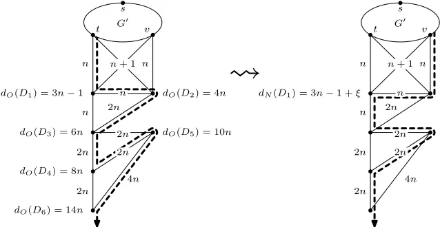
Proof.By means of a reduction, we will show that such an approximation algo-rithm could be used to solveRHP.
Let (G′, P) be an input instance forRHP, whereG′ = (V′, E′),|V′|=n+1,
s, t ∈V′, andP is a Hamiltonian path froms to t. We construct a complete weighted graphG= (V, E, c) as part of an input for thelm-∆-DlTSPas shown
in Figure 6: We set V =V′∪ {D1, . . . , D6} and, for any edge e between two vertices v1, v2 ∈V′, c(e) = 1, if e∈ E′, andc(e) = 2 otherwise. To the other edges, assign costs as depicted in Figure 6, and maximal possible costs to the non-depicted edges, and set the deadlinesdO(Di) according to Figure 6.
Pick some suitable 0< δ <1 and 0< α <1 such that α 2+δ ≥
1
2−ε. We use the zigzag construction defined in Lemma 8 with parametersX = 10n,g= 2n,
ζ= 2,k≥(n+ 7) α
1−α, and γ≥
2kn+10n
δ to obtain the graphGO of our input instance. This guarantees 2kn+ 10n≤δγandk≥α(k+n+ 6).
The given optimal Hamiltonian tour C in GO starts in s, uses the given Hamiltonian path inG′ tot, and afterwards follows the sequenceD
1, D2, D3,
D4, D5, D6. Hence, it reachesD6in time 13n. Following the zigzag construction, this leads to a cost of at least 10n+ k−23+ζg+kγ. In GN, we change the deadline for D1 to dN(D1) = 3n−1 +ξ for someξ≥1.C remains a feasible solution. If G′ contains a Hamiltonian path from s to some vertex v 6= t, an optimal solution uses this path and follows the sequenceD2, D1, D3, D5, D4, D6. This solution reachesD6 in time 10n. By Lemma 8, this cycle costs 10n+ (k+ 2ζ−4)g+ 2γ.
IfG′ does not contain any Hamiltonian path to such a vertexv,Cremains the optimal solution in the case where ξ = 1. If ξ ≥ 2, an optimal solution follows P to t and afterwards uses the sequence D2, D1, D3, D4, D5, D6. This solution reachesD6 in time 12n+ 1> X+g. By Lemma 8, we obtain a cost of 10n+ (k−3
2 +ζ)g+kγ. This leads to a ratio of at least 10n+ (k−3
2 −2)2n+kγ 10n+ (k+ 4−4)2n+ 2γ >
kγ
2kn+ 10n+ 2γ > kγ
(2 +δ)γ = k
(2 +δ) ≥
α
2 +δ(k+n+ 7)≥(
1
2 −ε)|V| . Hence, a polynomial-time (12−ε)|V|-approximation algorithm could be used
to solveRHP.
Theorem 8.Let ε > 0. There is no polynomial-time 12−ε|V| -approxi-mation algorithm for the subproblem of lm-∆-DlTSP where one deadline is
decreased by ξ≥1 unlessP =N P.
Proof idea.The proof can be done in a way similar to the proof of Theorem 7. The relevant construction is illustrated in Figure 7. Details will be given in a
journal version of this paper.
G′ s
t v
n
n n
n 2n n nn+ 1+ 1 n
n
n−1 n
dN(D2) = 3n−ξ
G′ s
t v
n
n n
n 2n n nn+ 1+ 1 n
n
n−1 n
dO(D1) = 4n dO(D2) = 3n
dO(D3) = 5n dO(D4) = 7n
dO(D5) = 6n
[image:19.612.141.470.89.266.2]dO(D6) = 9n
Fig. 7. Decreasing a deadline: If the deadline for the vertexD2 is decreased, the old optimal solution (depicted on the left-hand side) becomes infeasible. IfG′ contains a Hamiltonian path fromstov, we obtain the depicted new optimal solution. If no such Hamiltonian path exists, the new optimal solution must followD2, D1, D3, D5, D4, D6.
4 Conclusion
In this work, we have introduced and successfully applied the concept of reusing optimal solutions when input instances are locally modified. In the case of metric TSP, we are able to improve on the previously-known upper bound of 1.5, as achieved by Christofides’ algorithm (applied to the new instance, ignoring the given optimal solution), with non-trivial extensions to the near-metric case. As for TSP with deadlines, which is remarkably hard [6], we have been able to reestablish almost all known lower bounds on the approximability of its variants in the setting of local modifications.
As an open problem, we state the question how hard it is to approximate
lm-k-∆β-DlTSP. Another open problem is whether the NP-hardlm-∆-TSP
is also APX-hard.
References
1. T. Andreae: On the traveling salesman problem restricted to inputs satisfying a relaxed triangle inequality.Networks38, 2001, pp. 59–67.
2. T. Andreae, H.-J. Bandelt: Performance guarantees for approximation algorithms depending on parameterized triangle inequalities. SIAM Journal on Discrete Mathematics8, 1995, pp. 1–16.
4. H.-J. B¨ockenhauer, J. Hromkoviˇc, R. Klasing, S. Seibert, W. Unger: Approxi-mation algorithms for TSP with sharpened triangle inequality.Information Pro-cessing Letters 75, 2000, pp. 133–138.
5. H.-J. B¨ockenhauer, J. Hromkoviˇc, R. Klasing, S. Seibert, W. Unger: Towards the notion of stability of approximation for hard optimization tasks and the traveling salesman problem.Theoretical Computer Science 285, 2002, pp. 3–24.
6. H.-J. B¨ockenhauer, J. Hromkoviˇc, J. Kneis, J. Kupke: On the parameterized approximability of TSP with deadlines.Theory of Computing Systems, to appear. 7. H.-J. B¨ockenhauer, J. Hromkoviˇc, J. Kneis, J. Kupke: On the approximation
hardness of some generalizations of TSP.Proc. SWAT 2006, to appear.
8. H.-J. B¨ockenhauer, S. Seibert: Improved lower bounds on the approximability of the traveling salesman problem.RAIRO Theoretical Informatics and Applica-tions 34, 2000, pp. 213–255.
9. N. Christofides: Worst-case analysis of a new heuristic for the travelling salesman problem. Technical Report 388, Graduate School of Industrial Administration, Carnegie-Mellon University, Pittsburgh, 1976.
10. J.-F. Cordeau, G. Desaulniers, J. Desrosiers, M. M. Solomon, F. Soumis: VRP with time windows. In: P. Toth, D. Vigo (eds.):The Vehicle Routing Problem, SIAM 2001, pp. 157–193.
11. L. Forlizzi, J. Hromkoviˇc, G. Proietti, S. Seibert: On the stability of approxi-mation for Hamiltonian path problems. Algorithmic Operations Research 1(1), 2006, pp. 31–45.
12. H. Greenberg: An annotated bibliography for post-solution analysis in mixed integer and combinatorial optimization. In: D. L. Woodruff (ed.): Advances in Computational and Stochastic Optimization, Logic Programming, and Heuristic Search, Kluwer Academic Publishers, 1998, pp. 97–148.
13. N. Guttmann-Beck, R. Hassin, S. Khuller, B. Raghavachari: Approximation algo-rithms with bounded performance guarantees for the clustered traveling salesman problem.Algorithmica28, 2000, pp. 422–437.
14. J. A. Hoogeveen: Analysis of Christofides’ heuristic: Some paths are more difficult than cycles.Operations Research Letters 10, 1978, pp. 178–193.
15. J. Hromkoviˇc: Stability of approximation algorithms for hard optimization prob-lems.Proc. SOFSEM’99, Springer LNCS 1725, 1999, pp. 29–47.
16. J. Hromkoviˇc: Algorithmics for Hard Problems. Introduction to Combinatorial Optimization, Randomization, Approximation, and Heuristics. Springer 2003. 17. M. Libura: Sensitivity analysis for minimum Hamiltonian path and traveling
salesman problems.Discrete Applied Mathematics 30, 1991, pp. 197–211. 18. M. Libura, E. S. van der Poort, G. Sierksma, J. A. A. van der Veen: Stability
aspects of the traveling salesman problem based on k-best solutions. Discrete Applied Mathematics 87, 1998, pp. 159–185.
19. Ch. Papadimitriou, K. Steiglitz: Some examples of difficult traveling salesman problems.Operations Research 26, 1978, pp. 434–443.
20. Y. N. Sotskov, V. K. Leontev, E. N. Gordeev: Some concepts of stability analysis in combinatorial optimization.Discrete Appl. Math.58, 1995, pp. 169–190. 21. S. Van Hoesel, A. Wagelmans: On the complexity of postoptimality analysis of