Face recognition using SIFT descriptors and binary PSO with velocity control

Face Recognition using SIFT descriptors and

Binary PSO with velocity control

Juan Andr´es Maulini, Laura Lanzarini

III-LIDI (Institute of Research in Computer Science LIDI) Faculty of Computer Science, National University of La Plata

La Plata, Buenos Aires, Argentina {jmaulini,laural}@lidi.info.unlp.edu.ar

Abstract. In this paper, a strategy for face recognition based on SIFT descriptors of the images involved is presented. In order to reduce the number of false positives and computation time, a selection of the most representative feature descriptors is carried out by applying a variation of the binary PSO method. This version improves its operation by a suitable positioning of the velocity vector. To achieve this, a new modi-fied version of the continuous gBest PSO algorithm is used. The results obtained allow stating that the descriptors can be successfully selected through the strategy proposed solving the problems initially mentioned.

Keywords : Face Recognition, SIFT descriptors, Swarm Intelligence, Binary PSO, Velocity Control

1

Introduction

Face recognition is a biometric technique that is widely used in various areas such as security and access control, forensic medicine, and police controls. It involves determining if the image of the face of any given person matches any of the face images stored in a database. This problem is hard to solve automatically due to the changes that various factors, such as facial expression, aging and even lighting, can cause on the image.

provided, and in Section 7 the results obtained are described. Finally, in Section 8 the conclusions obtained are presented.

2

Related work

There are currently various solutions to this problem that use SIFT descriptors. It has been shown [1] that using SIFT descriptors for the face recognition process is better than Eigenfaces and Fisherfaces algorithms. Training datasets were of various sizes, which allowed establishing that performance decreases as dataset size decreases. As regards the significant number of SIFT descriptors required for a reliable comparison, it was observed that, with a lower number of descriptors, performance is better than that obtained with Eigenfaces and Fisherfaces.

In order to tackle the issue of comparing very long feature vectors for all images in a database, a biased classification of the features that make SIFT descriptors, is proposed and used to reduce the length of SIFT descriptors used for face recognition [2]. Thus, the number of comparisons is reduced and the recognition process is faster. This process also filters out those descriptors that are irrelevant for face recognition, thus increasing recognition accuracy.

On the other hand, a face recognition algorithm that uses the binary PSO al-gorithm to explore the solution space for an optimum subset of features in order to increase recognition rate and class separation is presented in [3]. This algo-rithm is applied to feature vectors extracted using the Discrete Cosine Transform (DCT) and the Discrete Wavelet Transform (DWT).

3

Particle swarm optimization

3.1 Continuous particle swarm optimization

In PSO, each individual represents a possible solution to the problem and adapts following three factors: its knowledge of the environment (its fitness value), its previous experiences (its memory), and the previous experiences of the indi-viduals in its neighborhood [4]. In this type of technique, each individual is in continuous movement within the search space and never dies.

Each particle is composed by three vectors and two fitness values:

– Vectorxi= (xi1, xi2, . . . , xin) stores the current position of the particle

– Vector pBesti = (pi1, pi2, . . . , pin) stores the best solution found for the particle

– Velocity vector vi = (vi1, vi2, . . . , vin) stores the gradient (direction) based on which the particle will move.

– The fitness value f itness xi stores the suitability value of the current solu-tion.

The position of a particle is updated as follows:

xi(t+ 1) =xi(t) +vi(t+ 1) (1)

As explained above, the velocity vector is modified taking into account its expe-rience and environment. The expression is:

vi(t+ 1) =w.vi(t) +ϕ1.rand1.(pi–xi(t)) +ϕ2.rand2.(gi–xi(t)) (2)

wherew represents the inertia factor [5],ϕ1 andϕ2are acceleration constants,

rand1andrand2are random values belonging to the (0,1) interval, andgi repre-sents the position of the particle with the bestpBestfitness in the environment ofxi(lBestorlocalbest) or the entire swarm (gBestorglobalbest). The values ofw,ϕ1 andϕ2are important to ensure the convergence of the algorithm. For detailed information regarding the selection of these values, please see [6] and [7].

3.2 Binary particle swarm optimization

PSO was originally developed for a space of continuous values and it therefore poses several problems for spaces of discrete values where the variable domain is finite. Kennedy and Eberhart [8] presented a discrete binary version of PSO for these discrete optimization problems.

In binary PSO, each particle uses binary values to represent its current position and the position of the best solution found. The velocity vector is updated as in the continuous version, but determining the probability that each bit of the position vector becomes 1. Since this is a probability, the velocity vector should be mapped in such a way that it only contains values within the [0,1] range. To this end, the sigmoid function indicated in (3) is applied to each of its values.

v′

ij(t) =sig(vij(t)) = 1

1 +e−vij(t) (3)

Then, the particle position vector is updated as follows

xij(t+ 1) =

1if randij< sig(vij(t+ 1))

0if not (4)

whererandij is a number ramdomly generated by an uniform pdf in [0,1]. It should be mentioned that the incorporation of the sigmoid function radically changes the way in which the velocity vector is used to update the position of the particle. In continuous PSO, the velocity vector takes on higher values first to facilitate the exploration of the solution space, and then reduces them to allow the particle to stabilize. In binary PSO, the opposite procedure is applied. Each particle increases its exploratory ability as the velocity vector reduces its value; that is, whenvij tends to zero, lim

t→∞sig(vij(t)) = 0.5, thus allowing each binary

take on either value. On the contrary, when the velocity vector value increases, lim

t→∞sig(vij(t)) = 1, and therefore all bits will change to 1, whereas when the

velocity vector value decreases, taking negative values, lim

t→∞sig(vij(t)) = 0 and

all bits will change to 0. It should be noted that, by limiting the velocity vector values between−_{3 and 3,}sig(vij)∈_[0.0474,0.9526], whereas for values above 5,

sig(vij)≃1 and for values below−5,sig(vij)≃0.

4

Binary PSO with velocity control

Based on the observations of the behavior of the velocity vector in the binary PSO algorithm defined in [8], and on the importance of correctly calculating the probabilities that allow changing each binary digit, a modified version of the original PSO algorithm to modify the velocity vector is proposed.

Under this new scheme, each particle will have two velocity vectors,v1 andv2. The first one is updated according to (5).

v1i(t+ 1) =w.v1i(t) +ϕ1.rand1.(2∗pi−1) +ϕ2.rand2.(2∗gi−1) (5)

where the variablesrand1,rand2,ϕ1andϕ2operate in the same way as in (2). The valuespiandgicorrespond to theith binary digit of thepBesti andgBest vectors, respectively.

The most significant difference between (2) and (5) is that in the latter, the shift of vector v1 in the directions corresponding to the best solution found by the particle and the best global solution does not depend on the current position of the particle. Then, each element of the velocity vector v1 is controlled by applying (6)

v1ij(t) =

⎧

⎨

⎩

δ1j if v1ij(t)> δ1j

−δ1j if v1ij(t)≤ −δ1j

v1ij(t)if not

(6)

where

δ1j= limit1upperj−limit1lowerj

2 (7)

That is, velocity vector v1 is calculated with (5) and controlled with (6). Its value is used to update velocity vectorv2, as shown in (8).

v2(t+ 1) =v2(t) +v1(t+ 1) (8)

Vectorv2 is also controlled as vectorv1 by changinglimit1upperjandlimit1lowerj bylimit2upperj andlimit2lowerj, respectively. This will yieldδ2j, which will be used as in (6) to limit the values ofv2. Then, the new position of the particle is calculated with (4) using the values ofv2 as arguments of the sigmoid function. Puede consultarse [2] para ver los resultados de este m´etodo en comparaci´on con [9] y [8] al ser aplicado en optimizaci´on de funciones.

5

SIFT Descriptors

In [10], Lowe defined a method to extract features from an image and use them to find matches between two different views of the same object. These features, called SIFT (Scale Invariant Feature Transform) features, are invariant to image scale and rotation, and quite invariant to affine distortion, as well as changes in point of view and lighting. They are also highly distinctive.

The process to determine SIFT features for an image consists in four steps:

– First, the location of potential points of interest within the image is deter-mined. These points of interest correspond to the extreme points calculated from plane subsets of Difference of Gaussian (DoG) filters applied to the image at different scales.

– Then, the points of interest whose contrast is low are discarded. This is an improvement from the definition in [11].

– After this, the orientation of relevant points of interest is calculated.

– Using the previous orientations, the environment is analyzed for each point and the corresponding feature vector is determined.

As a result of this process, a set of 128-length feature vectors that can be com-pared with those from another image of the same object with a different scale, orientation, and/or point of view, is obtained.

This comparison can be done directly by measuring the distance and estab-lishing a similarity threshold.

More detailed information about this method is available in [10].

6

Face Recognition

In order to perform face recognition, the method proposed uses a minimum-size database formed by the subset of most representative SIFT descriptors. Thus, the computing time required to make the necessary comparisons and detection of false positives are reduced. This selection process is performed before the recognition process; therefore, it does not affect the response time for the end user. Subsection 6.1. details how to make this selection.

The recognition of a new face involves the following steps:

– Calculating the SIFT vectors corresponding to the input image

– Comparing each vector in the database with the set of vectors corresponding to the new face, matches being accumulated not by image but rather by the number of the person to whom the database vector corresponds.

– The new face will correspond to the person with the highest number of accumulated matches.

information corresponding to one person, or, even better, to one image. Thus, the calculation of the number of matches found would be faster.As regards the recognition of the new face, a minimum threshold of matches can be used to identify faces that have no matches in the database.

6.1 Building the database

The method begins by obtaining all SIFT descriptors corresponding to each in-put image. The selection of the most representative SIFT descriptors is carried out by applying a variation of the method described in section 4, based on sub-populations of particles. In this case, the number of sub-populations to use matches the number of images in the database.

The length of the position vector for each particle of a population is deter-mined by the number of SIFT descriptors of the corresponding image. Therefore, the length of particles from different populations can be different. That is, the vector of thejth_{particle in the subpopulation i, has the following form}

Xji= (x i

j1, xij2, . . . , xijmi) (9) wheremi is the number of SIFT descriptors of imagei and xijk is 1 if the kth SIFT descriptor must be included in the data base and 0 if not.

This speciation criterion allows calculating the movement of each particle using only the SIFT descriptors from one image. Thus, each population searches a different part of the solution space. The final solution is obtained by concate-nation the best individuals of each population. This can be expressed as follows

X= (Xbest1 , Xbest2 , . . . , X M

best) (10)

where M is the number of different images used to form the database and Xibest is the best individual in the ith subpopulation.

With respect to the usual parameters of PSO: In each iteration, the value of w decreases, as mentioned in [8] and elitism was used so that, if moving individuals does not allow at least maintaining the highest fitness value found thus far, the best individual of the previous iteration regains its previous position and the fitness value lost. The algorithm terminates when the maximum number of iterations was reached or when after a certain number of consecutive iterations the best fitness value has not changed.

6.2 Assessing the fitness value of each particle

In this section, the method used to measure the fitness value for each particle is described. An expression that helps reducing the number of false positives must be used. Therefore, its value increases when the selected descriptor has a match in an image of the corresponding subject, and it decreases when there are no matches.

BeXi

BeC1i

jk the total number of matches between the k

th _{SIFT descriptor of}

imagei and the rest of the images that correspond to the subject represented by imagei.

BeC2i

jk the total number of matches between the k

th _{SIFT descriptor of}

image i and the images that correspond to subjects other than that represented by imagei.

The fitness value of thejth_{particle of sub-populationiis calculated as}

F iti j =

m

k=1

xi

jk∗(α1∗C1jki −α2∗C2ijk) (11)

whereα1andα2are constants with values between (0,1) and represent the sig-nificance of each term within the expression. As said above,xi

jk is 1 if the kth SIFT descriptor must be included in the data base and 0 if not.

7

Results Obtained

Measurements were carried out using two databases obtained from [12]. The first of these is the YALE faces database, containing 165 images of 15 different subjects (11 images per person). Each image has a resolution of 320x243 pixels. The second database used was theAT&T faces database, containing 400 images of 40 people (10 images per individual). The size of each image is 112x92 pixels. The available images were divided in two parts: Subset of input images, whose descriptors will be selected by applying the method proposed in Section 5 and subset of test images that will be compared with the selected SIFT descriptors for recognition.

The initial SIFT descriptors for each image were determined with a threshold of 0.5, as recommended in [11]. In both cases, the parameters used by PSO were the following: Initial and final inertia values: 1.2 and 0.2, respectively; maximum number of iterations = 500,α1= 1/(number of input images),α2= 16/(number of input images).

Thirty-five independent runs of the process described in Section 6 were car-ried out, varying the percentage of images used to form the base. Figure 1 shows the average percentage of correct matches calculated over the test images. It can be seen that, in both cases, the selection of SIFT descriptors using PSO favors the recognition process and yields a higher success rate.

Fig. 1.Percentage of matches for test images using the method proposed (SIFT+PSO) and the original SIFT method for various percentages of images from the YALE and AT&T databases

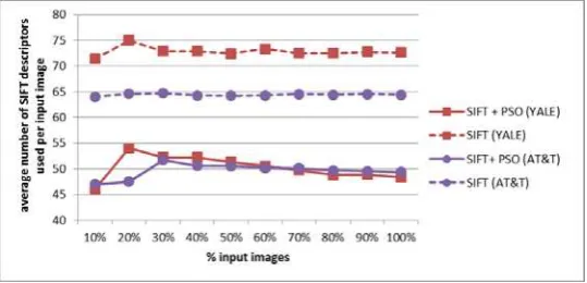
Finally, Figure 3 shows the average number of SIFT descriptors used for each image in the base. It can be observed that, even though the reduction in the number of descriptors is greater for YALE than for AT&T, it is significant in both cases.

Fig. 3.Average number of SIFT descriptors used for each image in the YALE and AT&T databases.

Figure 4 shows the original SIFT descriptors on the top row of images and descriptors selected by the proposed algorithm in the bottom row.

Fig. 4.SIFT descriptors of a person of the YALE database. The top row shows all descriptors found while the bottom row shows only the descriptors selected by the proposed method.

8

Conclusions

tests carried out with the YALE and AT&T databases have allowed reaching considerable reduction rates (50% in YALE and 25% in AT&T).

Even though the success rate for each test image using the base of descriptors selected with PSO is slightly higher than the one obtained with the process that uses all SIFT descriptors, the proportion of false positives is lower. Additionally, the smaller size of the database allows ensuring a clear reduction in the time needed for the recognition.

The parameters involved still need to be thoroughly analyzed in order to determine if a more precise adjustment would allow reducing the maximum number of iterations needed to reach an optimum selection of descriptors. The parallelization of the solution proposed also poses an interesting analysis.

References

1. Aly Mohamed. Face recognition using sift features. CNS186 Term Project, 2006. 2. Lanzarini L., L´opez J., Maulini J., and De Giusti A. A new binary pso with velocity

control. InAdvances in Swarm Intelligence, Part I, volume 6728, pages 111–119. Lecture Notes in Computer Science. Springer, 2011.

3. R. Ramadan and R. Abdel Kader. Face recognition using particle swarm optimization-based selected features. International Journal of Signal Processing, Image Processing and Pattern Recognition, 2(2):51–65, 2009.

4. J. Kennedy and R. Eberhart. Particle swarm optimization. IEEE International Conference on Neural Networks, IV:1942–1948, 1995.

5. Shi Y. and Eberhart R. Parameter selection in particle swarm optimization. 7th International Conference on Evolutionary Programming., pages 591–600, 1998. 6. Kennedy J. Clerc M. The particle swarm ˆA– explosion, stability and convergence

in a multidimensional complex space. IEEE Transactions on Evolutionary Com-putation., 6(1):58–73, 2002.

7. Van den Bergh F. An analysis of particle swarm optimizers. Ph.D. dissertation. Department Computer Science. University Pretoria. South Africa., 2002.

8. Kennedy J. and Eberhart R. A discrete binary version of the particle swarm algo-rithm. World Multiconference on Systemics, Cybernetics and Informatics (WM-SCI), pages 4104–4109, 1997.

9. Shoorehdeli M. Khanesar M., Teshnehlab M. A novel binary particle swarm opti-mization. 18th Mediterranean Conference on Control and Automation., pages 1–6, 2007.

10. David G. Lowe. Distinctive image features from scale-invariant keypoints. Inter-national. journal of computer vision, 60, 2004.

11. D.G. Lowe. Object recognition from local scale-invariant features.In International Conference on Computer Vision, pages 1150–1157, 1999.