A note on holography and phase transitions

(1)

Volume 2011, Article ID 917127,17pages doi:10.1155/2011/917127

Research Article

A Note on Holography and Phase Transitions

Marc Bellon,

1, 2

_{Enrique F. Moreno,}

3

_{and Fidel A. Schaposnik}

4

1_{UPMC Paris 06, UMR 7589, LPTHE, 75005 Paris, France} 2_{CNRS, UMR 7589, LPTHE, 75005 Paris, France}

3_{Department of Physics, Northeastern University, Boston, MA 02115, USA}

4_{Departamento de F´}ısica, Universidad Nacional de La Plata, C.C. 67, 1900 La Plata, Argentina

Correspondence should be addressed to Enrique F. Moreno,[email protected]

Received 23 February 2011; Revised 18 June 2011; Accepted 1 July 2011

Academic Editor: Anastasios Petkou

Copyrightq_{2011 Marc Bellon et al. This is an open access article distributed under the Creative}

Commons Attribution License, which permits unrestricted use, distribution, and reproduction in any medium, provided the original work is properly cited.

Focusing on the connection between the Landau theory of second-order phase transitions and the holographic approach to critical phenomena, we study diverse field theories in an anti de Sitter black hole background. Through simple analytical approximations, solutions to the equations of motion can be obtained in closed form which give rather good approximations of the results obtained using more involved numerical methods. The agreement we find stems from rather elementary considerations on perturbation of Schr ¨odinger equations.

1. Introduction

Much activity has been centered in the last few years on the application of the gauge/gravity

duality, originally emerged from string theory1–3, to analyze strongly interacting field

the-ories by mapping them to classical gravity. More recently such duality was successfully applied to describe, holographically, systems undergoing phase transitions like

superconduc-tors, superfluids, and other strongly interacting systems4–17 for a wider list of references

see e.g.,18.

In the holographic approach to the study of phase transitions one starts, on the gravity

side, with a field theory in asymptotically anti de SitterAdSspace-time with temperature

arising from a black hole metric, either introduced as a background or resulting from back reaction of matter on the geometry. Then, using the AdS/CFT correspondence, one can study the behavior of the dual field theory defined on the boundary, identify order parameters, and analyze the phase structure of the dual system.

Several models with scalar and gauge fields in a bulk which corresponds

(2)

nonlinear coupled diﬀerential equations that have to be solved require general application of numerical methods. In this way one often finds nontrivial hairy solutions that cease to

exist forT > Tc, whereT is the Hawking temperature associated with the black hole and

Tca critical temperature depending on the space-time dimensions and the parameters of the

model on the bulk.

The main point in this AdS/CFT based calculation is that the asymptotics of the solution in the bulk encodes the behavior of the QFT at finite temperature defined on the border. One finds in general a typical scenario of second-order phase transition. The critical exponents can be computed with a rather good precision and coincide with those obtained within the mean field approximation in a great variety of models.

It is the purpose of this paper to get an analytical insight complementing the numerical results, with a focus on the connection between the holographic approach and mean field theory for the calculation of critical exponents. To this end, it will be important to first

stress some connections, already signaled in 6, between the Landau phenomenological

theory of second-order phase transitions and the gauge/gravity approach. We will expose the importance of analyticity to explain the similitude in the results for relevant physical

quantitiescritical exponents, dependence of the critical temperature on the charge density,

and magnetic field, etc. in very diverse models. This will be done first by stressing the

relationship between the equations of motion and a Schr ¨odinger problem, so that usual perturbative techniques allow to prove the critical behavior. We then show that simple matching conditions lead to results that broadly agree with elaborate numerical calculations. It should be noted that our calculations assume that the backreaction of dynamical

fields is negligibleprobe approximationwhich is valid when the gauge coupling constant

is large. This approximation is useful to study the behavior near the phase transition which is precisely the domain we will analyze, comparing our analytical results with those obtained numerically. In fact, the holographic results we have previously obtained solving numerically the Einstein-Yang-Mills-Higgs equations of motion both considering the probe

approximation7and the case in which matter backreacts on the geometry5show that

when parameters are such that condensation takes place the solutions are very similar and the nature of the phase transition is identical.

With this in mind and using an analytic approach proposed in 8, we study the

equations of motion for diﬀerent models, showing how one can determine in a very simple

way the critical behavior of the systems defined on the border with a good agreement with numerical results.

2. Holography and Mean Field Results

In the Landau approach to second-order phase transitions one considers an order parameter

Oand assumes analyticity of the free energyF FT,O, which can be expanded in even

powers ofO

FT,O FF0F2TO2F4TO4· · ·. 2.1

The dependence of the order parameter onTis obtained by minimizingFas a function ofO.

The next step is to expand the coeﬃcientsF2 andF4, in powers ofT−Tc. To ensure stability

(3)

constants. In this way, one finds that the minimum ofF is atO 0 forT > Tc disordered

phasewhile forT < Tcone has

O ∼Tc−T1/2. 2.2

Let us give a brief description of gauge/gravity approach to phase transitions to connect it to the Landau theory. On the gravity side one considers a classical field theory

in a Schwarzschild-AdS black hole backgroundor one in which backreaction of fields on

an asymptotically AdS space leads to a black hole solution. The choice of such a geometry

is dictated by the fact that the warped AdS geometry prevents massive charged particles to be repelled to the boundary by a charged horizon and as a result a condensate floating over the horizon can be formed. To find such condensate one should look for nontrivial static solutions for the fields outside the black hole by imposing appropriate boundary conditions. The behavior of fields at infinity then allows to determine the dependence of the order parameter on temperature, identified with the Hawking temperature of the black hole.

Basically, the free energy F is identified with the minimum of the action in the

gravitational theory with prescribed boundary condition for the fields. Regularity of the fields at the horizon and smoothness of the background geometry, basic assumptions within the gauge/gravity duality, imply analyticity of this action. This is a first point of contact with Landau theory of second-order phase transitions leading to a mean field behavior. We will now see that if continuity and smoothness of fields are imposed in the region between the horizon and infinity, the mean field behavior found using a numerical approach is reproduced with a good precision, as can be seen following a very simple analytic approach proposed in

8which we apply below for diﬀerent models.

3. The Abelian Higgs Model in

d

Space Dimensions

Dynamics of the system is governed by the action

S

dd1_x_g

−1

4FµνF

µv₋_∇

µ−iAµΨ

2

−m2_|_Ψ_|2_. _3.1

The background metric is the standard AdSd1-Schwarschild black hole

ds2₋frdt2 1

frdr

2_r2_dx

idxi, i1,2, ..., d−1,

fr r2

1 − r

d h rd

,

3.2

withi 1,2, . . . , d−1 and we have chosen the AdS radius to be unity. Diﬀerent values for

the mass term can be considered9,10:m2 ₀_, ₋_{2 and}_m2 _m2

BF −9/4 ind 3 and

(4)

m2

BF < 0 marking the boundary of stability for a scalar field in AdS 19. The black hole

temperature is given by

T d

4πrh. 3.3

In order to look for simple classical solutions for this model one can propose the following ansatz:

Ψ _|Ψ_|ψr, Aµφrδµ0. 3.4

Imposing regularity of the solution at the horizonrrhone gets

ψrh drh

m2ψ′rh,

φrh 0.

3.5

Concerning the asymptotic behavior of the scalar potentialφand the scalar fieldψone has

ψ ψ− rλ−

ψ

rλ,

φµ− ρ

rd−2 · · · ,

3.6

with

λ_± 1

2 d±

d2₄_m2_. _3.7

According to the gauge/gravity correspondence,µcorresponds to the chemical potential in

the dual theory defined on the boundary andρto the charge density. Concerning the scalar

fieldψ, both falloﬀs are acceptable provided the following condition holds20:

−d

2

4 < m

2_<₋d2

4 1, 3.8

One can then pick eitherψ0 orψ−0 leaving a one parameter family of solutions so that

the condensate of the dual operatorOσ _{will be given by}

Oσψσ, 3.9

with the boundary condition written as

εσρψρ0, 3.10

(5)

It will be convenient for the analysis that follows to change variables according to

z rh

r , 3.11

so that the horizon is fixed atz1 and the boundary atz0. In terms of this new variable

z, the equations for the functions in ansatz3.4become

ψ′′− d−1z

d

z1−zd ψ

′

⎛

⎝ φ2

r2

h

1−zd2 −

m2

z2₁₋_zd

⎞

⎠ψ0, 3.12

φ′′₋d−3

z φ

′₋ 2ψ2

z2₁₋_zdφ0, 3.13

where the prime denotesd/dz.

Conditions3.5and3.6now read

ψ′₁ ₋

m2

d

ψ1 0,

φ1 0,

3.14

ψBz≃z→0DzλD−zλ−,

φBz≃z→0µ−qzd−2,

3.15

withD± r_h−λ± ψ±andqρ/r_hd−2.

In view of3.3, the system3.12-3.13only depends on the black-hole temperatureT

through the nonlinearφ2_ψ_{term in the scalar field equation}_3.12_{: this describes the coupling}

of the scalar to the electric potential and gives an eﬀective negative mass.

In the limitT → ∞the nonlinear term in3.12vanishes so that the equation becomes

linear with no nontrivial soliton solutions. Now, as already pointed out in11the coupling

of the scalar to the Maxwell field is responsible for producing a negative eﬀective mass forψ,

and this eﬀect becomes more important at low temperatures. This indicates that one should

expect an instability taking place at some point towards forming scalar hair. At such point, the

stabilizing eﬀect of them-term is overcome. If a nontrivial solution exists at low temperatures,

with an asymptotic behavior associated with a nonzero v.e.v. of an order parameterOψ

in the dual theory, it is natural to expect that a critical temperature Tc should exist such

that OψT>Tc 0. This was indeed verified numerically for diﬀerent values of the mass

mincluding the Breitenlohner-Freedman bound valueand various space-time dimensions

9,10.

Now, 3.12 for fixed potential φ can be viewed as a Schr ¨odinger equation with

zero energy: in order to have nontrivial solutions, the resulting potential has to adjust itself for the existence of a unique zero eigenvalue for every temperature below the critical one. In the vicinity of the critical point, the variation of the potential is linear in the

temperature variation, but quadratic in the normalization of the field through the eﬀect of the

(6)

proportional to some integral of the potential as can be seen from its variational evaluation:

with a suitable weight functionaz, the integral ofazψztimes the left hand side of3.12

gives the eigenvalue for a normalizedψand its variations are of second order with respect to

the variations ofψ. Fixingψto the eigenfunction forT Tc, the two sources of the variation of

this integral through the potential must compensate themselves, and one obtains aΔT ∝φ2

relation. It is precisely this type of behavior that has been found from the numerical solution

to the diﬀerential equations on the gravity side.

To go further in the analysis without resorting to a numerical analysis, we will consider

expansions of the fields in the bulk nearz1 andz0. Imposing the conditions of continuity

and smoothness of the solutions at a pointzmintermediate between the boundaryz0and

the horizonz1will give algebraic equations between the parameters of the solution.

For the solution near the horizonz1we have, up to orderz−12,

ψHz ψ0ψ1z−1 1

2ψ2z−1

2_,

φHz φ0φ1z−1 1

2φ2z−1

2_,

3.16

withψ0, ψ1, ψ2, φ0, φ1, φ2constants. The boundary conditions3.14atz1 imply

ψ1−

m2

d

ψ0,

φ0 0.

3.17

Substituting these values in3.16and using the diﬀerential3.12-3.13we can obtainφ2

andψ2as a function ofφ1andψ0. We get

ψHz ψ0

m2

d ψ01−z

2dm2_r2

hm4rh2−φ21

4d2_r2

h

ψ01−z2,

φHz −φ11−z 1 2

d−3−2ψ 2 0

d

φ11−z2.

3.18

As announced, imposing the conditions of continuity and smoothness at an

intermedi-ate pointzmallows to obtain a solution. Interestingly enough, as first observed in8the result

of this crude approximation is quite stable with respect to the intermediate point, so we will

consider the casezm1/2. This can be understood from the fact thatψis the ground state of

a Schr ¨odinger equation, so that it cannot have nodes: additional terms in the expansion ofψ

should rapidly fade away.

We will first analyze the boundary conditionD₋ 0, so we have the set of equations

ψH ₁ 2 ψB ₁ 2

, ψ′_H

₁

2

ψ_B′

₁ 2 , φH ₁ 2 φB ₁ 2

, φ′_H

₁

2

φ′_B

₁

2

,

(7)

to be solved forψ0,φ1,D, andµ. We obtain

ψ₀2 d

2d1

16d−2Bq2d_d₋₅_r

hA

rhA ,

D

2λ−1₄_d_m2

dB2 ψ0,

φ1−

rhA B ,

µ 1

2d2

8dqB2d_r

hA B

3.20

for simplicityDis written in terms ofψ0. Here

A

16d2_λ

m4λ2 2dm265λ,

Bλ2.

3.21

Using the AdS/CFT dictionary3.9, we can identify the v.e.v.Oof the operatorO dual

to the scalar field with the asymptotic coeﬃcientψ,O ≡ψ rλ_h D. Now, one can write

D or ψ0 since they are proportional as a function ofT d/4πrh. Remembering that

qρ/rd−2

h one has

ψ₀2 d5−d

2

_T

c T

d−1

1−

_T

Tc

d−1

, 3.22

where we have defined

Td−1

c

24−d_d₋₂

5−d4π/dd−1 B

Aρ. 3.23

We then have, for the order parameter

OCd

_T

Tc

√d2₄_m2₁_/₂

1−

_T

Tc

d−1

, 3.24

with

Cd

4dm2

λ2

_d

2π

λ₅₋_d

8d

1/2

. 3.25

One can see from27 that forT close toTc one has the typical second-order phase

transition behaviorO ∝1−T/Tc. Note thatTc ∝ρ1/d−1in agreement with the change

(8)

Our results for the critical temperature, as inferred from 3.23–3.25 in the cases

d 3, 4, m2 ₋₂ _with _z

m 1/2 are Tc 0.15ρ1/2 and Tc 0.2ρ1/3, respectively.

They can be compared with those obtained using a diﬀerent analytical approximation based

on perturbation theory near the critical temperature. For the case m mBF, we obtain

Tc 0.12ρ1/2 andTc 0.25ρ1/3 21,22in very good agreement with the exact numerical

results,Tc 0.15ρ1/2 andTc 0.25ρ1/3. One can conclude that there is a good quantitative

agreement between the three sets, which is not much aﬀected by the choice of the pointzmin

the method. This last fact was already observed in8for the particular cased3 compared

with the numerical results given in9.

4. Non-Abelian Gauge Field in

d

3 Space Dimensions

We now consider the case of an SU2Yang-Mills theory in 31 dimensional Antide

Sitter-Schwarzschild background, as a prototype for the gauge/gravity duality in the case of pure

gauge theories12,13. The action is

S₋1

4

d4xgF_µνa Faµν, 4.1

with the field strength defined as

F_µνa ∂µAaν−∂νAaµgǫabcAbµAcν, a1,2,3. 4.2

Writing the gauge field as an isospin vector

A A1, A2, A3 Aa_µdxµ, 4.3

we consider the following ansatz for solving the equations of motion:

AJrdteˇ3−KrρdϕeˇρKrdρeˇϕ, 4.4

whereris the radial variable in spherical coordinates and

xρcosϕ,

yρsinϕ.

(9)

The background metric is

ds2₋_frd2_t 1

frd

2_r_r2 _dx2_dy2_, _4.6

with

fr r2

1−r

3

h r3

. 4.7

In terms of thezvariable defined in3.11the equations of motion read

1−z3K′′ 1

r2

h

K2− J

2_z2

1−z3

K,

J′′z 2 r2

h

JzK2_z

1−z3 .

4.8

At the horizonz 1,J must vanish, so we have the following expansions for the

fields, up to orderz−12,

KHz K0K1z−1 1

2K2z−1

2_,

JHz J1z−1 1

2J2z−1

2_.

4.9

Using the equations of motion4.8, the coeﬃcientsK1,K2, andJ2can be written in terms of

K0andJ1as

KHz K0−

K3 0

3r2

h

z−1 −J

2

1K0r_h26K30r2h3K50

36r4

h

z−12,

JHz J1z−1−

J1K02

3r2

h

z−12.

4.10

At thez0 boundary one has the asymptotic expansions

KBz

C1

rhz ,

JBz D0 −

D1

rhz ,

4.11

where D1 can be associated with the charge density. Coeﬃcient C1 in 4.11 should be

(10)

parameter is related to a vector fieldAi, the associated theory on the border is a p-wave

superconductor13.

As in the scalar field case, we will match both solutions at an intermediate point which

we again choose aszm1/2,

KH ₁ 2 KB ₁ 2

, K′_H

₁

2

K′_B

₁ 2 , JH ₁ 2 JB ₁ 2

, J′

H ₁ 2 J′ B ₁ 2 , 4.12

and solve these equations forK0,J1,C1, andD0. From the first two identities4.12, we obtain

C1 4

3rhK0

K3 0

9rh

,

J1

−48r_h222K₀23 K₀4/r_h2

4.13

we choseJ1<0 soJz>0.

Substituting these values in 4.12, we can obtain K0 as the root of the following

polynomial inK2₀:

3

r2

h

K₀840K₀6207r_h2K₀4486r_h4K2₀−9r_h2 D₁2−48r_h40. 4.14

This equation implies thatK₀2vanishes as

K₀2 D

2

1−48rh4

54r_h2 O D

2

1−48rh4

2

. 4.15

Finally, introducing the temperatureT3/4πrh, we can write

K2₀ 128π

2 81 T4 c T2 1− _T c T 4

forT near Tc, 4.16

where

T_c2 3

√ 3

64π2D1. 4.17

Then, forT close toTc, we have the typical second-order phase transition behavior forC1

OK ∝

1−T/Tc, in good agreement with12,13. Our numerical value forTcfrom4.17,

Tc/

D1 0.091, can be compared with the numerical value obtained in 13,Tc/

D1

(11)

5. The

d

3 Scalar Case in the Presence of an Applied Magnetic Field

We will consider here a system with dynamics governed by the action3.1in the d 3,

m2 ₋_{2 case, when an external magnetic field}_H _{is applied. This corresponds to the case}

where the background metric is an AdS31magneticallycharged black hole14,15:

ds2₋frdt2 1

frdr

2_r2_dx

idxi, i1,2,

fr r

2

L2 −

M

r

H2

r2 .

5.1

Thefr 0 condition for having event horizons gives a quartic algebraic equation with 4

roots which can be explicitly written in terms of surds. There are two complex conjugate roots

which we will callr1 andr2 and two real rootsr3 < r4. We will then callrh ≡r4the external

black hole horizon. TakingL1 from here on, one has

rh 1

261/3

⎛

⎝B

12M

B −B

2 ⎞

⎠, 5.2

where

B

831/3H2

D9M21/3 2

1/3_D₉_M21/3_, _D₈₁_M4₋₇₆₈_H6_. _5.3

The actual form of the other rootsraa1,2,3is not necessary since one will only need the

standard relationships between roots and coeﬃcients

r1r2r3−rh,

r1r2r1r3r2r3r_h2,

r1r2r3

H2

rh ,

5.4

together with the relation

H2

r4

h

−M

r_h3 10. 5.5

The Hawking temperature associated to the black hole is

T f

′_r_h

4π

1

4π

3rh− h

2

r3

h

(12)

In terms of the variablezrh/r, the equations of motion read

ψ′′z dfrh/z/dz

frh/z

ψ′z r

2

h z4

φ2_z

frh/z2

2

frh/z

0,

φ′′z−2 ψ

2_z

frh/z

φz

r_h2 z4

0,

5.7

whereψz ≡ ψrh/zandφz ≡ φrh/z but from now on, the tilde will be omitted. In

terms of the new variables, we have

f rh z

rh z

2

1−z1−r1z1−r2z1−r3z,

dfrh/z/dz

frh/z

−2−M

z3_/r3

h

2H2_z4_/r4

h

z1−z1−r1z1−r2z1−r3z

,

5.8

whererara/rh , a1,2,3.

The boundary conditions for system5.7at the horizon are

φ1 0, 5.9

ψ′1 2rh

3rh−H2/r_h3

ψ1, 5.10

while asymptotically one has

ψz D1zD2z2,

φz µ−

_ρ

rh

z.

5.11

For the solution of system5.7near the horizon, we have the expansions, up to order

z−12,

ψHz ψ0ψ1z−1 1

2ψ2z−1

2_,

φHz φ0φ1z−1 1

2φ2z−1

2_,

5.12

withψ0,ψ1,ψ2,φ0,φ1, andφ2constants. Using5.10we get

φ0 0,

ψ1 2rh

3rh−H2/r_h3

ψ0.

(13)

Substituting these values in5.12and using the diﬀerential equations, we can obtainφ2and

ψ2as functions ofφ1andψ0. We get

ψz ψ0

2r4_h

H2₋₃_r4

h

ψ01−z−

r4

h

8r4

hrh2φ12−12H2

4H2₋₃_r4

h

2 ψ01−z2,

φz −φ11−z

r4

hψ02φ1

H2₋₃_r4

h

1−z2.

5.14

As before, we impose matching conditions atz1/2:

ψH ₁ 2 ψB ₁ 2

, ψ′_H

₁

2

ψ_B′

₁ 2 , φH ₁ 2 φB ₁ 2

, φ′_H

₁

2

φ′_B

₁

2

,

5.15

and solve forψ0,φ1,D2, andµ. We look for solutions withD1 0 andD2corresponding to

the order parameter of the 21 system defined on the boundary. We obtain

φ1−2Rrh, H,

µ H

2_ρ/r

h2Rrh, H−r_h43ρ/rhRrh, Hψ₀26

2H2₋₃_r4

h

,

ψ₀2

3r_h4−H2_ρ/r

h−2Rrh, H

2r4

hRrh, H

,

D2

88r_h8−φ2

1rh6−68H2rh416H4

ψ0

4H2₋₃_r4

h

2 ,

5.16

where

Rrh, H

7rh8−6H2rh42H4

r6

h

. 5.17

The equation forψ2

0 in terms of the dimensionless variableurh/

√

Htakes the form

ψ2₀

3u4₋₁ _ρ/H₋₂₂_/u4₋₆₇_u4

2u4₂_/u4₋₆₇_u4

(14)

with the temperature5.6given by

T

√

H

1

4π

3u− 1

u3

. 5.19

The minimum value that u can take is the one for which T 0, u 3−1/4, and

corresponds to the condition 33_M4₂7_H6_{. From this, we see that in order to have a nontrivial}

solution the following inequality should hold:

H≤ ρ

22/u4₋₆₇_u4. 5.20

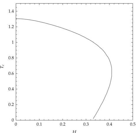
The maximum of the r.h.s. is attained forum 2/71/8 > u0 so that there is a critical value

Hcof the magnetic field beyond which no nontrivial solution exists,

Hc0.41ρ. 5.21

Using5.18-5.19, one can determine the critical temperatureTcas a function ofH.

We give inFigure 1the resultingTcTcHcurve. Interestingly, we find that in the range

Hc> H >

ρ

22/u4

0

−67u4

0

0.327ρ, _5.22

the curveTcHbecomes double valued so that a nontrivial solution only exists in the range

Tc2 > T > Tc1. According to the gauge/gravity dualityD2should be identified with the order

parameter,OψD2. We obtain the following expression:

D2

5u4₋₂

6u4₋₂

ρ/H−22/u4₋₆₇_u4

u2₂_/u4₋₆₇_u41/4 .

5.23

Note thatD2becomes negative foru0 < u <2/51/4or, equivalently, for 0< T <0.0316

√

H.

However, whenH → 0 the numerator and denominator coeﬃcients ofD2 that multiplyψ0

cancel out. This is consistent with the result of the nomagnetic field model.In fact, we have

checked that the results of both models,H0,d3, andm2 ₋_{2, are identical. We present}

in Figure 2curves for D2 as a function of temperature for diﬀerent values of the external magnetic field.

The results are qualitatively in agreement with those described in14,15where the

(15)

0.5 0.4

0.3 0.2

0.1 0

0 0.2 0.4 0.6 0.8 1 1.2 1.4

Tc

[image:15.600.185.416.93.319.2]

H

Figure 1:The phase diagram ofTcagainst the magnetic fieldH. The condensed phaseD2/0corresponds to the lower left part below the line. The critical temperature decreases as the magnetic field grow up to the critical valueHc.

0.6 0.8 1 1.2

T 0.05

0.1 0.15 0.2 0.25 0.3

D

2

Figure 2:A plot of the order parameterD2as a function of temperatureT. The charge density isρ1. The dashed line corresponds to a magnetic fieldH 0.1, the dash-dot one toH 0.2, and the solid one to H0.3.the critical value isHc0.6.

6. Summary and Discussion

We have analyzed a number of models which have been proposed to study phase transition through the AdS/CFT correspondence. The common feature of all three models we discussed was that the space time bulk geometry was an Anti de Sitter black hole. Although the

dynamical field content was very diﬀerent—a charged scalar coupled to an electric potential,

[image:15.600.188.412.379.521.2]

(16)

On general grounds, we were able to explain why the highly symmetric ans¨atze generally used produce the critical behaviors seen in mean field theory or the Landau approach. Founded on basic principles as the connection between the equations of motion and the Schr ¨odinger equation, we clarify the similarity between several relevant quantities along a variety of models. In particular we showed that resorting to simple matching conditions, we obtain closed form solutions that significantly agree with the results obtained by numerically solving the exact set of equations of motion. This uncovers the important role played by analyticity to explain the universal behavior of certain physical constants.

The method seems to work very well near the critical temperature, though it deviates

from the numerical results as we approachT → 0. In this regime our approach should be

refined.

Alternative analytic calculations have been recently presented in23,24 where the

phase transition vicinity is studied solving the equations of motion in terms of a series expansion near the horizon. Although the approach in these works is close to the one

proposed in 8 and applied here, the possibility in the latter of varying the intermediate

pointzmat which the matching is performed allows to obtain better solutions at fixed order

N in the expansion, as already pointed out in24. As we have seen that, in the matching

approach, the problem reduces to find the solution of an algebraic equations system and this can be done, to the order we worked here, in a straightforward way. Increasing the order will of course complicate the algebraic system but in view of its main features, it can be handled by a simple computational software like Mathematica, at least for the next few

orders. For a large-order expansion the method followed in references23,24seems to be

more appropriate.

Although the matching method works very well near the critical temperature, it

deviates from the numerical results as T approaches 0. In this regime the method should

be refined. In particular it is to be expected that taking into account the quantum fluctuations of the gravity theory, one should be able to go beyond mean field approximation results.

Also, one should consider generalized Lagrangianslike the St ¨uckelberg one considered in

16 leading to various types of phase transitionsfirst or second order with both mean

and nonmean field behavioras parameters are changed. There is also the possibility that

including fermions in the bulk model could substantially change the critical behavior of the

theory in the bulksee25and references therein. The simplicity of the approach presented

here, not requiring refined numerical calculations, should be an asset when trying to explore these more complex situations.

Acknowledgment

F. A. Schaposnik is associated with CICBA.

References

1 J. Maldacena, “The largeN limit of superconformal field theories and supergravity,”Advances in Theoretical and Mathematical Physics, vol. 2, no. 2, pp. 231–252, 1998.

2 S. S. Gubser, I. R. Klebanov, and A. M. Polyakov, “Gauge theory correlators from non-critical string theory,”Physics Letters B, vol. 428, no. 1-2, pp. 105–114, 1998.

(17)

4 S. S. Gubser, “Phase transitions near black hole horizons,”Classical and Quantum Gravity, vol. 22, no. 23, pp. 5121–5143, 2005.

5 A. R. Lugo, E. F. Moreno, and F. A. Schaposnik, “Holography and AdS4 self-gravitating dyons,”

Journal of High Energy Physics, vol. 2010, no. 11, pp. 1–19, 2010.

6 N. Iqbal, H. Liu, M. Mezei, and Q. Si, “Quantum phase transitions in holographic models of magnetism and superconductors,”Physical Review D, vol. 82, no. 4, Article ID 045002, 2010.

7 A. R. Lugo, E. F. Morenob, and F. A. Schaposnika, “Holographic phase transition from dyons in an AdS black hole background,”Journal of High Energy Physics, vol. 2010, no. 3, article 013, 2010.

8 R. Gregory, S. Kanno, and J. Soda, “Holographic superconductors with higher curvature corrections,”

Journal of High Energy Physics, vol. 2009, no. 10, article 010, 2009.

9 S. A. Hartnoll, C. P. Herzog, and G. T. Horowitz, “Building a holographic superconductor,”Physical Review Letters, vol. 101, no. 3, 4 pages, 2008.

10 G. T. Horowitz and M. M. Roberts, “Holographic superconductors with various condensates,”

Physical Review D, vol. 78, no. 12, Article ID 126008, 2008.

11 S. S. Gubser, “Breaking an Abelian gauge symmetry near a black hole horizon,”Physical Review D, vol. 78, no. 6, Article ID 065034, 2008.

12 S. S. Gubser, “Colorful horizons with charge in anti-de Sitter space,”Physical Review Letters, vol. 101, no. 19, p. 191601, 4, 2008.

13 S. S. Gubser and S. S. Pufu, “The gravity dual of ap-wave superconductor,”Journal of High Energy Physics, vol. 2008, no. 11, article 033, 2008.

14 E. Nakano and W.-Y. Wen, “Critical magnetic field in a holographic superconductor,”Physical Review D, vol. 78, no. 4, Article ID 046004, 2008.

15 T. Albash and C. V. Johnson, “A holographic superconductor in an external magnetic field,”Journal of High Energy Physics, vol. 2008, no. 9, article 121, 2008.

16 S. Franco, A. M. Garc´ıa-Garc´ıa, and D. Rodr´ıguez-G ´omez, “Holographic approach to phase transitions,”Physical Review D, vol. 81, no. 4, Article ID 041901, 5 pages, 2010.

17 S. A. Hartnoll, C. P. Herzog, and G. T. Horowitz, “Holographic superconductors,”Journal of High Energy Physics, vol. 2008, no. 12, article 015, 2008.

18 G. T. Horowitz, “Introduction to holographic superconductors,”Lecture Notes in Physics, vol. 828, pp. 313–347, 2011.

19 P. Breitenlohner and D. Z. Freedman, “Stability in gauged extended supergravity,”Annals of Physics, vol. 144, no. 2, pp. 249–281, 1982.

20 I. R. Klebanov and E. Witten, “AdS/CFT correspondence and symmetry breaking,”Nuclear Physics. B, vol. 556, no. 1-2, pp. 89–114, 1999.

21 G. Siopsis and J. Therrien, “Analytic calculation of properties of holographic superconductors,”

Journal of High Energy Physics, vol. 2010, no. 5, article 013, 2010.

22 G. Siopsis, J. Therrien, and S. Musiri, “Holographic conductors near the Breitenlohner-Freedman bound,”http://arxiv.org/abs/1011.2938.

23 C. P. Herzog, “Analytic holographic superconductor,”Physical Review D, vol. 81, no. 12, Article ID 126009, 11 pages, 2010.

24 F. Aprile, S. Franco, D. Rodr´ıguez-G ´omez, and J. G. Russo, “Phenomenological models of holographic superconductors and Hall currents,”Journal of High Energy Physics, vol. 2010, no. 5, article 102, 2010.

25 T. Faulkner, N. Iqbal, H. Liu, J. McGreevy, and D. Vegh, “Holographic non-Fermi-liquid fixed points,”

(18)

Submit your manuscripts at

http://www.hindawi.com

Hindawi Publishing Corporation

http://www.hindawi.com Volume 2014

High Energy PhysicsAdvances in

World Journal

Fluids

Journal of

Atomic and Molecular Physics

Journal of

http://www.hindawi.com Volume 2014 Condensed Matter Physics

Optics

International Journal of

http://www.hindawi.com Volume 2014 Advances in

Astronomy

International Journal of

Superconductivity

Statistical Mechanics International Journal of Hindawi Publishing Corporation

Gravity

Astrophysics

Journal of

http://www.hindawi.com Volume 2014 Physics

Research International

http://www.hindawi.com Volume 2014 Solid State PhysicsJournal of Computational Methods in Physics

Journal of

Soft Matter

Hindawi Publishing Corporation http://www.hindawi.com

Aerodynamics

Journal of

Volume 2014

Photonics

Journal of

A note on holography and phase transitions

Research Article