Individual heterogeneity in the returns to schooling: instrumental variables quantile regression using twins data

www.depeco.econo.unlp.edu.ar

Individual Heterogeneity in the Returns to Schooling: Instrumental

Variables Quantile Regression using Twins Data

Omar Arias, Kevin F. Hallock y Walter Sosa Escudero

INDIVIDUAL HETEROGENEITY IN THE RETURNS TO SCHOOLING: INSTRUMENTAL VARIABLES QUANTILE REGRESSION

USING TWINS DATA

Omar Arias

University of Illinois at Urbana-Champaign Champaign, Illinois

Kevin F. Hallock

University of Illinois at Urbana-Champaign Champaign, Illinois

Walter Sosa

Universidad Nacional de la Plata La Plata, Argentina

March 29, 1999

INDIVIDUAL HETEROGENEITY IN THE RETURNS TO SCHOOLING: INSTRUMENTAL VARIABLES QUANTILE REGRESSION

USING TWINS DATA

ABSTRACT

Considerable effort has been exercised recently in estimating mean returns to education while carefully considering biases arising from unmeasured ability and measurement error. Some of this work has also attempted to determine whether there are variations from the “mean” return to education across the population with mixed results. In this paper, we use recent extensions of instrumental variables techniques to quantile regression on a sample of twins to estimate an entire family of returns to education at different quantiles of the conditional distribution of wages while addressing simultaneity and measurement error biases. We test whether there is individual heterogeneity in returns to education against the alternative that there is a constant return for all workers. Our estimated model provides evidence of two sources of heterogeneity in returns to schooling. First, there is evidence of a differential effect by which more able individuals become better educated because they face lower marginal costs of schooling. Second, once this endogeneity bias is accounted for, our results provide evidence of the existence of actual heterogeneity in market returns to education consistent with a non-trivial interaction between schooling and unobserved abilities in the generation of earnings. The evidence suggests that higher ability individuals (those further to the right in the conditional distribution of wages) have higher returns to schooling but that returns vary significantly only along the lower quantiles to middle quantiles. In our final approach, the resulting estimated returns are never lower than 9 percent and can be as high as 13 percent at the top of the conditional distribution of wages, thus providing rather tight bounds on the true return to schooling. Our findings have meaningful implications for the design of educational policies.

JEL Classification: C14, I2, J24, J31

Key Words: Returns to Education, Human Capital, Heterogeneity, Quantile Treatment Effects,

Instrumental Variables.

Omar Arias Kevin F. Hallock Walter Sosa

Department of Economics Department of Economics Department of Economics

University of Illinois University of Illinois Universidad Nacional de

1206 South 6th Street 1206 South 6th Street la Plata

Champaign, IL 61820 Champaign, IL 61820 La Plata, Argentina

217 333-0120 217 333-4842 541 553 9983

1. Introduction

The causal relation between education and earnings has been one of the most heavily and

carefully explored subjects in empirical work in labor economics. The many empirical and theoretical

difficulties associated with the analysis of such a relationship have been approached with a remarkable

variety of econometric tools on diverse data sets. A well known problem that arises in these studies is

that it is difficult to isolate the causal impact of additional education on earnings. One must be sure that

what is claimed to be the return to additional schooling is not being distorted by the effect of other

relevant but unobserved factors that may be related to schooling. More specifically, if unobserved

“abilities” in the generation of earnings or family background factors are related to the level of

schooling attained, ignoring such a link would lead to incorrect inferences regarding the causal effect

of education.

There are several reasons why economists and policy makers are interested in obtaining

accurate measures of the earnings premium associated with acquiring more education. From a

“private” point of view, under certain conditions, it provides a measure of the “return” to investment in

additional schooling. From a social standpoint, the return to education could give an indication of the

relative scarcities of people with different levels of education and hence it may provide a guide for

educational policies.1 _{(See Psacharopoulos and Ng, 1994 for a cost-benefit formulation).}

In this paper we are interested in exploring whether people with different levels of “ability”

obtain different returns to education. Specifically, we provide unique empirical evidence to address two

of the important questions carefully laid out in Card (1995a): “what is the causal effect of education?”

and “is there evidence of individual heterogeneity in returns to education?”.

Our concept of “ability” refers to those marketable unobservable factors that make up an

individual’s initial endowment of human capital and translate into higher earnings. These may vary

across families as well as individuals.

as “IQ”, for which measures can be constructed using test scores. Most studies estimate the mean

return to education which may be interpreted as the return to additional schooling for an individual with

mean ability. This is a sensible characterization when the return to education is constant across levels

of (unobserved) ability so that any increase in schooling affects earnings of individuals that are

observationally identical in the same way. In this case, ability and education do not interact in the

generation of human capital; both factors have independent contributions to the accumulated stock.

Instead we take education and ability as two separate factors in the generation of human

capital which interact in a non-trivial, unknown way. On the one hand, if we think that ability and

education are substitutes in the generation of human capital, then marginal returns to the accumulation

of human capital are decreasing in ability and hence education contributes relatively more to low ability

individuals. On the other hand, we might think that ability and education are complements in the

generation of human capital, that is, education has an additional indirect effect on human capital and an

indirect effect that comes through the interaction with ability that increases its otherwise constant

contribution to earnings. We therefore want to investigate whether education induces a pure location

shift in the distribution of earnings, or some more intricate change. In the language of the empirical

literature on program evaluation, we are interested in whether the response to the treatment

(education) varies across individuals. In this case, the mean return to education is only one summary of

a richer pattern of ways that education affects people's earnings.

In order to explore this issue, we face several methodological and empirical limitations. First,

we do not observe ability, so we cannot model its relationship with education explicitly by including

additional regressors based on the former and estimate interaction effects with the later.2 _{Second, even}

though we can make some a priori conjectures about the relationship between ability and education,

we do not want to impose unrealistic and unnecessary restrictions on this interaction. In the above

examples, the return to education would be a monotonic function of the level of ability, but we see no

reason to impose such a restriction. We want our empirical model to be exploratory and informative

about the nature of this relationship. Third, education is not randomly assigned to individuals so we

cannot treat the attained level of education as a predetermined variable. The optimal level of education

may be determined endogenously as function of the level of ability and other factors such as family

background. Fourth, it is well documented (e.g. Griliches, 1977, and Ashenfelter and Krueger, 1994)

that the schooling variable is typically measured with error, which may introduce additional biases in

conventional estimates that do not account for this possibility.

The interaction between ability and education studied in this paper has been directly or

indirectly explored in some previous work but, as stressed in Card (1995a), there is little evidence in

the empirical literature to support (or reject) the hypothesis of homogeneity in the returns to education.

Ashenfelter and Rouse (1998) analyze an expanded version (three additional years) of the sample of

genetically identical twins used in Ashenfelter and Krueger (1994). They exploit the presumed

similarity of twins and the availability of multiple measures of schooling to explicitly model the link

between family ability and education parametrically, while addressing the measurement error and

endogeneity biases using standard panel data methods. They find some evidence of the existence of a

benefit more from additional schooling. More recently, Conneely and Uusitalo (1998) investigate the

question of heterogeneous returns in the context of a random coefficients model of wage

determination. They use data on ability test scores and family background variables on a sample of

Finnish men and parameterize potential heterogeneity in the mean return to education by interacting

these factors with education. They find stronger evidence of variations in returns to education most of

which, nevertheless, cannot be explained by observable individual heterogeneity.

We believe these fully parametric approaches impose strong restrictions on the structure of

heterogeneity in returns to education. In this paper we use instrumental variables quantile regression

methods on the recent sample of 858 genetically identical twins from Ashenfelter and Rouse (1998).

Quantile regression methods allow us to estimate returns to schooling for individuals at different

quantiles of the conditional distribution of earnings which we view as reflecting the distribution of

unobservable ability. Unlike the above approaches which explicitly concentrate on the effect of

education on the conditional mean of earnings and parameterize variations in returns through proxies

for ability, quantile techniques allow us to freely characterize the effect of education on the whole

conditional distribution of earnings.

Although he does not treat the ability-education interaction explicitly, Buchinsky’s (1994)

analysis of the U.S. wage structure, using Current Population Survey (CPS) data and censored

quantile regression methods, shows that returns to education in the U.S. increase dramatically over the

quantiles of the conditional distribution of wages. Mwabu and Schultz (1996) also use quantile methods

on a sample of 3117 men for South Africa and obtain varying returns across quantiles that they

interpret along the lines explored in this paper. Nevertheless, the results of these studies should be

interpreted with caution since they do not handle the problems of measurement error or endogeneity

bias. The finding of heterogeneous returns may simply reflect a variable ability-based endogeneity

bias: more able individuals, facing lower marginal costs of schooling choose to acquire more education

and appear to have higher marginal returns to education. See also Fitzenburger and Kurz (1998) for

an interesting approach to studying earnings data using quantile regression and data from Germany and

Machado and Mata (1999) who study wage inequality in Portugal.

The availability of twins data (with multiple measures of schooling) allows us to deal with the

endogeneity of education arising from measurement error while indirectly controlling for any ability

bias arising from “family effects”.3 We also use testing procedures based on quantile regression

statistics to formally test for the presence of heterogeneity in the returns to education. Our approach is

semiparametric in the sense that it imposes relatively weak parametric structure on the relationship

between earnings and education. Minimal structure is imposed on the key relationship of interest: the

interaction between education and ability in the generation of earnings.

As in all the other previous twins literature, our estimates rely crucially on the assumption that

any absolute ability bias is due to unobservable family (inherited) factors. In a recent paper, Bound

and Solon (1998) criticize the estimates of returns to education based on twins data questioning the

validity of this assumption. If this assumption fails, our estimates can be thought to provide a whole

family of bounds on the causal effect of education on earnings.

The paper is outlined as follows. In section 2, we specify a simple structural model of schooling

choices closely based on Becker (1967), Card (1995a) and Ashenfelter and Rouse (1998). We extend

the model by being less restrictive in the parameterization of heterogeneity. Section 3 briefly describes

the data and outlines previous estimates of the mean return to schooling. In section 4, we present the

details of model specification and estimation, develop tests for heterogeneity in returns to schooling,

and discuss the results. Section 5 discusses policy implications of our findings and concludes. In the

appendix, we provide a brief discussion of quantile regression methods and the testing procedures used

in the paper and highlight their usefulness for investigating heterogeneity.

2.

The Basic Model and its Interpretation in the Quantile Regression Context

In this section we specify a simple structural model that highlights the main aspects of the problem.

Following Ashenfelter and Rouse (1998) and Card (1995a) our model is based on the Becker (1967)

model of investment in education with explicit focus on the following questions: 1) What is a sensible

way to think about the link between ability and education? 2) Are returns to education homogeneous

across the population? If not, how can we model the source of this heterogeneity and how can it be

explored? 3) Why is quantile regression an appropriate tool to explore these types of effects which

involve unobservable factors in a non-trivial way? 4) How does the availability of twins data allows us

to deal with measurement error and simultaneity bias in the quantile regression framework?

2.1 The Basic Model

The starting point is the utility maximization problem of the i-th twin in family j:

(

)

(

(

)

)

(

)

ij

r

S

h A

S y S

Y U S

,

, , ln ,

max = ε − (1)

The first term consists of a human capital production function which receives as inputs education (Sij),

an unobservable “ability” variable (Aj), and a random twin specific disturbance (εij) observed by the

individual but not by the econometrician from an unspecified common continuous distribution function

f_ε. This term reflects how education, ability and the idiosyncratic shock interact in the generation of

earnings (Yij). The second term measures the explicit and implicit (opportunity) costs of acquiring

more education. It depends on education as well as family factors such as wealth or tastes for

education summarized by (rj). We will think of (Aj) as a measure of unobservable “family effects”

that cause individuals from different families to earn different wages. These “family effects” could

capture differences in family specific initial human capital, differences in the quality of schooling as

well as differences in labor market connections across families.4 The individual random component

captures factors such as individual specific ability and risk taking that allow otherwise identical

individuals from the same family to earn different wages.

The schooling decision of an individual in the j-th family depends at the margin on the balance

of the marginal benefits and costs from additional schooling given his or her endowment of ability and

family background. If utility is globally concave with respect to (Sij), there will be a unique level of

education S*_ij

=

choices will potentially differ both among individuals of different families due to “family effects” and

between twins from the same family due to the idiosyncratic disturbance in the earnings function. This

is precisely the well known endogeneity of ability bias that has historically haunted estimates of the

returns to schooling. The acute problems that the potential correlation between (Aj, rj, εij) and the

observed choices of (Sij) pose to estimation of even the simplest linear empirical earnings functions

were lucidly discussed by Griliches (1977, 1979).

The advantage of using data on earnings and education from a sample of twins to estimate the

returns to schooling comes from exploiting the common components of the unobservable ability

variable across twins. Let vij = γ Aj + εij which corresponds to our concept of “ability”. A simple

specification that allows us to highlight the important issues is

(

)

0 ,

ij cS ij

S j r ij ij ij S ij S S

Y

U _{ij ij} =β +φ ν +ν − − −

where

e

(

)

represents the earnings function and

2

5 . 0 _ij ij

jS cS r

e

the cost function.5 _{In this case the marginal condition for a maximum solution to (1) is:}6

Since twins tend to attend the same school, differences in the quality of schooling are only relevant across families.

5

This is an extension of Rosen (1973) . 6

ij j ij S

ij

ij MC r cS

MB

ij= ≡ +

+ ≡

≡β β0 φ (2)

where

ij S

φ denotes the derivative of φwith respect toSij.

Following Becker (1967), βij is interpreted as the return to schooling, which at this point may

depend on the level of education and unobservable ability. The function φ governs the process by

which ability affects the rate at which human capital is accumulated. Thus, assuming differentiability,

in (2) at the optimal level of schooling we have that:

( )

where φS,v denotes the cross-partial second derivative of U with respect to Sijand νijand captures

how ability affects the return to education. As long as φS,v≠ 0 the return to education will not be

constant across individuals (of the same education level). Differing abilities alter returns so that there

exists a family of returns to education. This is precisely what we mean by heterogeneity in the returns

to education. Note that the standard specification and estimation of Mincer equations assumes φS,v =

0 implicitly which implies that education and ability are “perfect substitutes” in the production of human

capital. If φS,v > 0 ability enhances the productivity gains of acquiring an additional year of education,

while if φS,v < 0 high ability individuals face lower returns to investment in education. Both cases are

possible since we do not need to require φS to be monotonic in vij. Similarly, for c > 0, marginal cost is

increasing in education and depends on rj which implies variations in the rate at which individuals of

the same family substitute schooling for future earnings. Since higher ability parents will tend to have

higher earnings and acquire more education, these differences may in turn reflect differences in the

wealth or tastes for education across families. We expect Aj is negatively correlated with rj to

capture the intuitive notion that individuals from more able families face lower disutilities of schooling.

As discussed by Ashenfelter and Rouse (1998), a crucial condition to identify the return to

schooling from within-family variation in schooling levels is that any differences in schooling between

twins of the same family are due to optimization or measurement errors that are uncorrelated with the

earnings disturbance. That is, we need to assume that:

ij j ij S u

S*

=

+

where the uij are iid errors over i and j from an unspecified continuous distribution function fu, and are

independent of the εijand true schooling levels. This amounts to assuming that any within twins

difference in the marginal benefit from schooling do not affect their optimal schooling choices. Note

that twins from different families can still choose different education levels due to differences in family

ability.7 _{Recently Bound and Solon (1998) have raised questions on the plausibility of this assumption.}

Nevertheless, using the same data we use in this work, Ashenfelter and Rouse (1998) carried out a

variety of tests which provide evidence consistent with the hypothesis that schooling choices among

twins are uncorrelated with unobservable determinants of earnings.8

Note that (3) implies that differences in observed schooling levels in the population arise from

two sources. First, individuals may have differing returns to schooling (due to differing Ajs). Second,

individuals may have different marginal rates of substitution between schooling and future earnings (rj)

due to differences in the implicit marginal costs of schooling. Thus, for the utility specification

considered we have that at

S

j j A S j ij

ij

A r

A S

U

∂ ∂ φ ∂ ∂

∂

−

= ,

2

(5)

which determines the rate at which an individual of the same family can substitute ability and education

in the generation of utility. When (5) is negative the marginal rate of substitution between ability and

education is decreasing with the level of ability: the same amount of schooling substitutes less ability as

an individual becomes gradually more educated. The opposite is true if it is positive. Since we expect

the correlation between Aj and rj to be negative, then in the case that φS,A > 0 we have that both

effects work in the direction of enhancing the ability-based endogeneity bias by which more able

individuals are the more educated.

2.2 The Empirical Framework

Integrating MBij over Sijwe obtain the log-linear human capital production function for which we adopt

the following empirical specification:

( )

(

)

ln α λ β φ (6)

often called the Mincer (1974) equation. We denote observed family specific variables (age (for

twins), race), Fj. Xij stands for observed individual specific characteristics other than education such

as union participation and marital status, and α, λ, γ, β are the corresponding coefficients. This

equation together with (4) determine the joint distribution of earnings and education.

7

This implies that individuals have better information than the econometrician but that this is still imperfect. 8

Our empirical model aims to estimate the returns to schooling from data on wages and

education from a sample of twins while accounting for four features of empirical measurements from

this distribution: i) the stylized log-linear relationship between observed wages and education,9 _ii)

heterogeneity in the distribution of earnings conditional on education, iii) the endogeneity of observed

education levels due to unobservable ability, and iv) measurement error in observed schooling choices.

First note that the presence of φ introduces a potential non-linearity in the above log-linear

Mincer equation. Nevertheless, because of the positive correlation between βij and education, equation

(6) is not necessarily inconsistent with a linear relationship between log wages and education. For

instance, as pointed out by Card (1995a), if for a given level of ability, wages are a concave function of

education, the data for the population as a whole could still trace out a convex relationship between

wages and education.10 _{In order to keep consistency with the documented log-linearity of wages and}

education we shall assume that φS,A is independent of education. We discuss the issues involved in

(ii)-(iv) below.

2.2.1 Quantile Regression and Unobserved Heterogeneity.

Provisionally, let us ignore the endogeneity ability bias and measurement error in education for

now, ie., assume that Sijis independent of family effects and can be treated as exogenous. The optimal

schooling model outlined above implies that unobserved ability induces heterogeneity in the joint

distribution of earnings and schooling. Letting Z= (Fj, Xij), we see that OLS on (6) gives a measure of

( ) (

)

(

)

E ∂ β δ

∂ ln , / = + : the return to education for an individual with mean ability as

pointed out by Card (1995a). In this case the labor market cannot yet be well characterized by a single

rate of return to education. Ashenfelter and Rouse (1998) focused on the conditional mean of the

distribution of wages to obtain different estimates of βij for the case that φij = δ Aj Sij so that

heterogeneity takes the simple linear heteroskedastic form:

( )

∂

ln

Y

/

∂

S

≡

β

=

β δ

+

A

Here δ captures the effect of ability on the return to education (ie., (3)). They estimate δ by

including as an additional regressor an interaction term between education and the average education

of a pair of twins from family j which from (4) can be taken as a proxy for ability in that family. A

negative δ means that returns to education are lower for high ability individuals, which in our model is

interpreted as a decreasing marginal rate of substitution between ability and education. In this case low

ability individuals benefit more from additional education. An analogous interpretation holds for positive

δ. The drawback of this approach is that the resulting estimate of the heterogeneity parameter (and

thus of the βjs) relies on a full parameterization of the interaction between education and unobserved

ability Aj. The same limitation applies to the recent attempt of Conneely and Uusitalo (1998) of

estimating heterogeneous returns to education based on conditional mean wage functions. The

approach makes it very difficult to separately identify the effect of ability on the marginal benefit of

schooling, as reflected in estimates of the interaction coefficient that are in general statistically

insignificant. We want to be able to characterize the family of returns to education without making

such restrictive parametric assumptions.

The regression quantiles of Koenker and Bassett (1978) provide a more general approach to

characterizing the effect of education on different percentiles of the conditional distribution of wages,

thus allowing us to explore and estimate heterogeneity in the returns to schooling. Specifically, a zero

conditional quantile restriction on the error vij implies that the effect of education on the τ-th quantile of

Yij conditional on the observables in (6) is:11

(

)

(

(

)

)

₍

₎

S

Z

G

S

S

Z

Q

S

S

Z

Y

Q

,

,

,

τ

β

∂

∂

β

β

∂

∂

=

+

=

+

≡

where Gv is some transformation of the distribution function of abilities in the population since we have

assumed that the marginal return to education is independent of education. Thus, by estimating quantile

regressions for different values of τ one can obtain consistent estimates of the whole family of returns

to education functions reflecting the distribution of abilities across individuals (Note that in the absence

of heterogeneity, β₀ =β_τ for all τ . The interaction between education and ability can then be

explored by comparing β(τ)s at different quantiles τk and τj, for i≠ k. Moreover, a robust test of the

hypothesis of heterogeneity (βk ≠ β for some k) can be based on a test of whether the estimated

coefficients for the returns to education differ across quantiles. That is, using the test for

heteroskedasticity proposed by Koenker and Bassett (1982). Unlike the prior approaches, this does not

require strong parametric restrictions on the type of interaction between ability and education.

As indicated previously, the findings of heterogeneous returns by Buchinsky (1994) and

Mwabu and Schultz (1996) based on quantile wage equations come close to such a characterization.

Nevertheless, this work does not address the problems of endogeneity bias and measurement error in

education, and does not structurally model the source of heterogeneity. Since (3) implies that in general

Qτ(νij|Sij) ≠ 0, quantile regression on a Mincer equation like (6) would yield inconsistent estimates of

the family of returns to education just as OLS fails to deliver a consistent estimate for the mean return.

Specifically, he considers the case where

φ

=

b S

−

0 5

k S

2

.

In fact, varying returns to education can be a result of an endogeneity bias that varies across quantiles

of the conditional distribution of wages rather than evidence of actual ability-based differences in the

market marginal returns to education. We now discuss how the data on twins allow us to more

carefully uncover the evidence for “true” heterogeneity in the returns to education while addressing

both the simultaneity and measurement error biases.

2.2.2 The Endogeneity of Schooling

In our model, individuals from higher ability families (Aj) become better educated due to

lower marginal costs of schooling. As noted before, if ability and schooling are “complements” in the

generation of earnings, then the higher returns to education for the more able enhance this endogeneity

bias in schooling. In the previous literature on estimation of the returns to education using twins data

this problem has been addressed in two ways. One approach is to treat Ajas an unobserved random

family effect and focus the interest on obtaining unbiased estimates of the structural coefficients βj

measuring the returns to education. This can be accomplished by directly estimating a “fixed effects

model” based on the (within) differenced equation corresponding to (6) for each pair of twins across

families. Since (2) and (6) imply that

E

(

ξ

∆

S

,

∆

X

)

=

0

ξj= ε1j −ε2j, OLS on differenced data yields consistent estimates of the mean return to education. This

is the strategy adopted by Ashenfelter and Krueger (1994) and Ashenfelter and Rouse (1998) to deal

with the ability bias in the OLS context.

One might naïvely consider quantile regression on a differenced Mincer equation since then

Qτ(∆ξij | ∆Sij) = 0. Nevertheless, there is a fundamental drawback with this approach. Although

differencing in the least squares context can be shown to be equivalent to a fixed effects estimator, in

the context of quantile regression, this is not the case. Estimates of quantile regression education

coefficients from a differenced equation would reflect the effect of education on the quantiles of the

conditional distribution of the difference in wages between a pair of twins across families, rather than

the effect on the difference in the quantiles of the corresponding conditional wage distributions. Since

quantiles of the sum of two random variables are not equal to the sum of the quantiles of each random

variable at a given τj, when differencing in quantile regression, the order of the individuals matters.

Thus, it is not possible to recover the estimates obtained using data on levels on an equation like (6)

from the estimates of quantile regressions on differenced data. Moreover, the natural attempt to

estimate the fixed effects model including family specific dummies is also futile in this case given the

unavoidable ambiguity surrounding the identification of the fixed effects at any given quantile with only

An alternative approach is to try to parameterize and estimate the endogeneity (omitted ability

variable) bias explicitly including some proxy for unobserved ability as an additional regressor when

estimating equation (6). As long as the proxy can account for most of the endogeneity bias, this

approach also allows us to obtain consistent estimates of the returns to education. Ashenfelter and

Krueger (1994) and Ashenfelter and Rouse (1998) also provide such estimates of the returns to

education and the resulting endogeneity bias (to which they refer as a “selection effect”). The model

of optimal schooling choices outlined in section 2 suggests that we use measures of the education of a

twin’s sibling, the average education of the twins, or father’s education as an additional regressor to

control for any “family” effect that affect the absolute level of earnings. This is the approach we use

in our empirical work and we label the resulting specifications as “family effects” models. The

coefficients on these variables provides us with alternative quantile specific estimates of the ability bias

in the estimates of returns to schooling.

2.2.3 Measurement Error in Education

The information contained in the available twins data provides an interesting way to address

the problem of measurement error in reported schooling which can arise because of the recall errors

common in survey data. This is specially important since from the work of Griliches (1977) it is well

known that the attempt to control for any absolute ability bias using family education variables to proxy

for family effects exacerbates already existing biases.

As reported in Ashenfelter and Krueger (1994) and Ashenfelter and Rouse (1998), twins are

asked to report on the education level of their sibling and of their parents. Letting

S

report of the n-th family member, we can expect such cross-reports to satisfy (3) so that:

S

=

S

+

u

where unjk denotes iid measurement errors over i n and j.

These cross-reports of each family member’s education can then be employed as instruments

using recent extensions of instrumental variable methods to quantile regression (see the appendix).

Moreover, the availability of multiple reports allows us to relax the classical assumption of uncorrelated

measurement errors in the own-reports of a twin. This can occur if a twin that overreports his own

education level is also more likely to overreport the education level of his sibling and of his parents.

Following Ashenfelter and Krueger (1994) and Ashenfelter and Rouse (1998), we also estimate

quantile regression models that assume correlated measurement errors in education.

The data used in this paper were collected over a span of five years at four meetings (August

of 1991, 1992, 1993, and 1995) of the Annual Twins Festival in Twinsburg Ohio. Many of the

questions are similar to questions asked in the Current Population Survey (CPS) with some

twins-specific questions added. As Ashenfelter and Krueger (1994) and Ashenfelter and Rouse (1998)

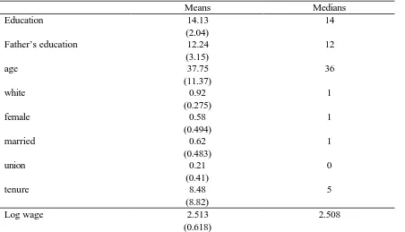
show, the mean characteristics of the sample are quite similar to the population at large. Sample

characteristics are reported in Table 1. The sample we use has, on average, more years of education,

higher income, and is more likely to be female and white than the population at large. Ashenfelter and

Krueger (1994) also note these similarities and differences.

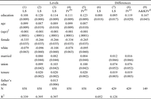
Table 2 reports regression results employing econometric specifications similar to Ashenfelter

and Krueger (1994), Ashenfelter and Rouse (1998) and Rouse (1997) who focused on estimating the

mean return to education. We briefly present these results for three reasons. First to highlight (as in

the previous literature) the importance of considering both ability and measurement error biases in

estimating mean returns to education. Secondly to document the mean return to education using these

specific data. Finally, Table 2 provides a summary of the data and specifications that will be extended

to the quantile regression framework below.

The first five columns of Table 2 estimate very simple empirical earnings equations. Column 1

of Table 2, reports the simple least squares regression of the log of earnings on age, (age)2, a gender

indicator equal to 1 if the individual is female and an indicator equal to 1 if the respondent is white. This

model is estimated using all 858 respondents for which we have complete data. In column 2 we have

included additional controls for marital status, union coverage and tenure. As usual, there is a positive

seniority profile, and the female indicator is large and negative. The white indicator is also negative (an

anomalous result also found in Ashenfelter and Krueger, 1994, Ashenfelter and Rouse, 1998, and

Rouse, 1997) but is not statistically different from zero. The return to education estimated in column

(1) is 10.8%. As we have stated earlier and as is well documented in Griliches (1977) and Ashenfelter

and Krueger (1994), this estimate is potentially upward biased due to unobserved ability and downward

biased due to measurement error. A great deal of effort has been focused on determining the “true”

return to education after accounting for these biases. Card (1995a) provides an important and

interesting summary of a set of papers that find that simple least squares estimates seem to be

downward biased12_.

The other columns in table 2 present the results of estimating additional, yet similar,

specifications that address these ability and measurement error biases. Column 3 presents the

family specific ability. We can see that this reduces the return to education from 12% (column 2) to

11.4% and that the coefficient on father’s education is significant, thus consistent with an upward

ability bias. On the other hand, comparison of the OLS and IV estimates reported in columns 3 and 5

suggest the presence of a slight downward bias in the mean return due to measurement error in

education. Instrumental variables results from a specification similar to column 5 that includes father’s

education (not reported) are also consistent with this view.

Columns 6-9 estimate models where the data are “differenced.” Each unit of observation is

created by subtracting the given variable from his or her twin’s. Column 6, then, is simply the

difference in log twins wage on the difference in reported education for the twins. Column 8 contains

our mean estimate that is most closely related to Ashenfelter and Krueger’s (1994) final estimate

(re-printed as column 9). This is the differenced model using instrumental variables where the instrument

is the first twin’s report of the second twin’s education minus the second twin’s report of the first’s.

Our resulting estimate of the return to education 11.9% is not unlike the least squares estimate of

10.8% but is considerably lower than Ashenfelter and Krueger’s (1994) similarly specified estimate of

16.7%. Rouse (1997) using the same four years of data that we use (Ashenfelter and Krueger, 1994

use only one year) points out that “Unlike the results in Ashenfelter and Krueger, I find that the

within-twin regression estimate of the effect of schooling on the log wage is smaller than the cross-sectional

estimate, implying a small upward bias in the cross-sectional estimate.” She further notes, however,

that her results and those of Ashenfelter and Krueger are not statistically different and suggests that

the difference is perhaps due to sampling error.

In the next section we turn attention away from estimating the mean return toward estimating

and testing the implications of our simple theoretical model of heterogeneity in the returns to schooling.

4. Estimation Details and Empirical Results

This section outlines in more detail the framework we use to develop our empirical models and

formal tests for heterogeneity in the returns to education under the presence of endogeneity and

measurement error biases. In Sections 4.1 to 4.5 we detail the specifications we use, describe the

empirical results and the strategies for testing equality in the returns to schooling across various

quantiles. See the Appendix for a brief technical description of the methods used.

The main focus of this paper is on estimating and testing for heterogeneity in returns to

schooling across quantiles of the conditional wage distribution while addressing endogeneity and

measurement error biases. To this end, we will consider four empirical models: 1) the levels model

without instrumental variables, 2) the levels model with instrumental variables, 3) the family effects

model without instrumental variables, and 4) family effects model with instrumental variables. The

ideas behind these models roughly follow the empirical work in the recent literature on twins

(Ashenfelter and Krueger, 1994, Ashenfelter and Rouse, 1998, and Rouse, 1997) replicated in Table 2.

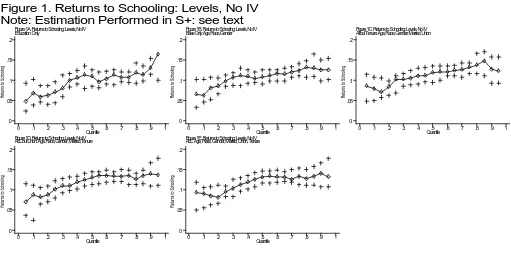
4.1 Levels Model Without Instrumental Variables

Figure 1 presents the quantile regression estimates of the returns to education for the levels

model without instrumental variables. The β(τ)’s for the 5th to 95th quantiles are plotted in increments

of 0.05 and the figure is separated into five sub-figures according to the covariates included in the

estimation. In addition to controlling for education these plots control for A) education only, B) age,

race, and gender only, C) (“all” but tenure) controls for age, race, gender, married, and union, D) (“all”

but union) controls for age, race, gender, married, and tenure, and E) controls for age, race, marital

status, union, and tenure.

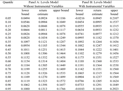
We focus our attention on the specification that includes all covariates (Figure 1E). The actual

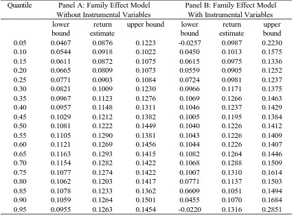
returns for each of the 19 quantiles are also reported in Table 3A, Panel A with 90% confidence

bounds for this specification (the confidence bounds are also reported in the figures). Recall that

homogeneity in returns would imply that the figures are flat. A cursory examination of the figures

suggests the presence of heterogeneity in the returns to education. The returns are, in general,

increasing for higher quantiles of the conditional distribution of wages. In particular, the median return

to education from Table 3A, panel A is 13.1% (compared to the mean return of 12% reported in

column 2 of Table 2). However there is a striking increase in the return from the low quantiles to

higher quantiles going from 9.2% at the 0.05 quantile to 13.1% at the median, after which the returns

essentially remain constant. Note also that the magnitude and the pattern of the estimates of the

returns to education remain remarkably similar across specifications (see figure 1). Also note that the

confidence bands in each figure within Figure 1 don’t include β_τ =β₀for any β₀. That is, for this

simple specification, the returns do not appear to be homogenous.

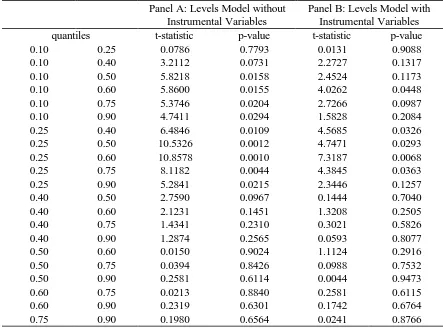
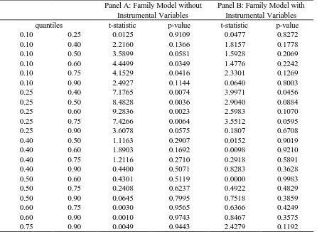
We test whether the observed differences are statistically significant across quantiles and

report the results of such tests in Table 3B, panel A. The tests confirm the visual impression. The tests

of equality of returns between the low quantiles and the middle quantiles, and between the low and

high quantiles reject the hypothesis of homogeneous returns at 1-2% significance levels. For example,

there is a statistically significant difference between the returns at the 0.10 and 0.50 quantiles

(t-statistic = 5.82, p-value = 0.016). Note, however, that the differences between the middle and higher

quantiles are not significant. Another way to see this is that Figure 1 flattens out in the right tail. These

education in the generation of earnings for those in the lower tail of the conditional distribution of

wages (i.e., the low ability), while for the upper tail marginal returns to education are higher but remain

constant.

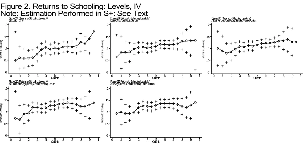
4.2 Levels Model with Instrumental Variables

Of course, the above results are still subject to the two main criticisms described by and

controlled for in Ashenfelter and Krueger (1994) and Ashenfelter and Rouse (1998) investigating the

mean return to education. We take the first step toward addressing these problems by estimating the

levels model using instrumental variables for the education variable to alleviate the measurement error

problem. We follow the previous literature and use twins #2’s report of twin #1’s own education (and

vice versa) as an instrument. These results are reported in Figure 2 which is arranged like Figure 1 in

that we report results for five different sets of covariates. Again, we have reported the returns to

education for the 19 quantiles 0.05 to 0.95 in Table 3A panel B with 90% confidence bounds for the

specification including all covariates.

The same general conclusions drawn from Figure 1 may be drawn from Figure 2. In

particular, failure to address the measurement error in education in the levels model does not seem to

create a significant downward bias in the estimated returns to schooling. After controlling for

measurement error in the levels model, we can still see evidence of heterogeneity in returns to

education with increasing returns at higher quantiles. Notice, however, that the standard error bands

are somewhat wider in the instrumental variables case so even if there are small differences, they are

unlikely to be significant.

We report tests of significance in the levels model with instrumental variables in Table 3B,

panel B. Here the results are largely consistent with those in the levels model without instruments,

supporting the visual impression of heterogeneous returns except that the tests cannot reject the

hypothesis of equality of returns between extreme quantiles due to higher standard errors of these

estimates. This might suggest that instrumenting affects the “true” schooling signal in own reported

education more sensibly for those at the tails of the conditional wage distribution. Overall, the findings

suggest that the bias that arises from measurement error in education in the levels models is not very

important. In the absence of endogenous ability bias, the estimates from the previous levels models

would provide relatively accurate measures of the family of returns to schooling.

4.3 Family Effects Model Without Instrumental Variables

This section and the one that follows repeats the analysis of sections 4.1 and 4.2 with the

in Section 2.2 above, the implementation of a quantile regression analogue of estimating an OLS fixed

effect or differenced model is problematic. Instead, in our quantile regression equivalent of a fixed

effects model we use the father’s level of education and the sibling’s education as proxies for the

family effect. We only report the results for the former.13 _{Essentially, we are re-doing the analysis}

reported in Figures 1 and 2 and Tables 3A and 3B with the additional covariate which is the father’s

schooling level. Note that even though we follow Ashenfelter and Rouse (1998) in the

parameterization of the endogeneity bias in this way, we do not parameterize the impact of the

interaction between ability and education on earnings. The novelty of our approach lies precisely in the

use of quantile regression techniques to explore this relationship based on the quantiles of wage

residuals that we interpret as capturing unobservable ability to generate earnings.

Figure 3 reports the results. Table 4A, panel A reports the returns to education for 19 quantiles

0.05 to 0.95 with 90% confidence bounds for the specification including all covariates. Clearly,

including the family effects has a substantial effect on the estimated returns. In general, the lines in

Figure 3 are lower than the corresponding ones in Figure 1, particularly at higher quantiles. This is

consistent with our expectation that part of the return to education is absorbed by the family effect

thus reflecting a positive endogeneity bias. This can be seen in the Appendix Figure which plots the

coefficient on father’s education and sibling’s education for the 19 quantiles. The estimates of the

endogeneity bias across different quantiles are in general increasing, though the precision of these

estimates is poor. Note that the sibling’s family effects models yield a slightly higher estimate of the

endogeneity bias, but the precision of the estimates is much poorer. This suggests that the findings of

Buchinsky (1994) of higher returns to education at higher quantiles and to a lesser extent those of

Mwabu and Schultz (1996) reflect in part a differential endogeneity bias in schooling choices of

individuals with different abilities rather than “true” differences in the marginal returns to education for

those in the upper tail of the conditional wage distribution.

Nevertheless, it is quite clear from Figure 3 that in each specification, though the quantile

curves of the estimated returns are flatter than in Figure 1, they are still generally increasing. These

patterns remain essentially intact when using sibling’s education as a proxy for family ability.

Therefore, although differences across quantiles are, no doubt, less significant, there still appears to be

some heterogeneity in the returns to education. This is confirmed by the tests we report in Table 4B

panel A which indicate rejection of the hypothesis of homogeneous returns in the middle quantiles.

Despite the apparent substantial differences in the estimated returns between extreme quantiles, poor

precision as reflected by the wider confidence bounds leads to insignificance test statistics.

4.4 Family Effects Model With Instrumental Variables

The problem with the estimates from the previous Section is that by including measures of

education to control for family effects, the potential bias arising from measurement error in schooling

levels is now aggravated since the cross-correlation between education levels (which is 0.75 among

siblings) washes away some of the “true” schooling signal in own-reported education levels. In this

Section we report the results of our best attempt to control for both the ability and the measurement

errors biases. This is the direct extension of section 4.2 except that we now use twin #2’s reports of

father’s education and of twin #1’s own report to instrument for potential measurement error in twin

#1’s report of father’s education and twin #1’s reported education, respectively (and vice versa). In

the case of sibling’s education we also estimated models that allow for correlation in the measurement

errors of a twins’ reports. Again we only report the results for the models using father’s education

since these results were very similar, except for the poorer precision of the estimates from the sibling’s

education models. In Figure 4, which we call the “family effects” models with instrumental variables,

the returns are somewhat sporadic. Note also that the confidence bands are wider, specially at the

extreme quantiles.

We report the actual returns and confidence intervals for the model with all variables in table

4, Panel B. A comparison with the non IV estimates of the analogous family effect model indicates

that the IV estimates are somewhat larger (consistent with a downward bias due to measurement

error) but only in the lower tail of the distribution of wage residuals. Considering the wider confidence

bounds on the IV estimates these differences are hardly significant. Moreover, although the family

effect model with instruments (Figure 4E) still suggests some mild heterogeneity in the returns to

education with higher returns at higher quantiles, the estimates are somewhat imprecise. In fact, when

we test (Table 4B, panel B) for differences across quantiles, only in the middle quantiles do we find

some evidence of heterogeneity in the returns (p-values between 5-10%). Once again it appears that

the attempts to deal with both the endogeneity bias and measurement error washes away most of the

“true” schooling signal of own reported education at the tails of the conditional wage distribution

leading to less precise estimates. From the Appendix Figures we can see in fact that the estimates of

the family effects based on both father’s education and sibling’s education are rather imprecise in the

instrumental variable models.

4.5 Do the Endogeneity and Measurement Error Biases Matter? Are Returns

Heterogeneous?

We now briefly summarize what we have learned from our empirical models that attempt to

document the existence of heterogeneity in the returns to schooling while dealing with the two well

known sources of biases. The results are summarized in Figure 5 which decomposes the differences in

the estimated returns to education obtained from the “all” covariates specification across our four

empirical models into the endogeneity bias and measurement error components.14_{Turning first to the}

measurement error problem, we see that comparison of the levels model non-IV vs. IV (see Figure

5A) and father's education model non-IV vs. IV (see Figure 5C) both reveal that the IV estimates

seem to be slightly higher than the non-IV case in the left tail, consistent with a slight downward bias

due to measurement error. The IV estimates actually appear to be lower than the non-IV at the high

quantiles (0.8-0.9) but this probably reflects the effect of noisier estimates at the tails.15_{So, one can}

conclude that the evidence suggests that failure to account for measurement error seems to create

slight downward biases in the estimates of the returns to schooling only at the lower quantiles, if at all.

But again, the IV estimates are less precise, particularly at the tails.

Does ability bias matter? Comparison of estimates from the levels models non-IV vs. father's

educ models non-IV (Figure 5D) and levels models IV vs. father's educ models IV (Figure 5B) are

revealing. First, the shapes of the curves are similar. There is an almost perfect overlap of the curves

in the lower quantiles. Beyond the 0.40th quantile, the family models' curves are slightly above, so

there is evidence of a slight upward ability bias in the right tail in models that do not account for

endogeneity of schooling choices.

More important for the key question addressed in this paper is the fact that the pattern of

return estimates is essentially unaffected by measurement error in both the levels models and all the

family effects models. There is a tendency for returns to increase monotonically along the lower tail of

the conditional wage distribution, returns then flatten out but tend to remain higher in the right tail.

These findings are supported by our formal tests and suggest that differential endogeneity bias does

not fully account for the patterns of heterogeneous increasing returns found in the base levels models.

Some of this heterogeneity does seem to reflect actual differences in the market returns to schooling

arising from a complementary relationship between education and ability which gives an advantage to

those at the top of the conditional wage distribution but also enhances earnings potential for low-wage

individuals.

4.6 Estimation results for other Covariates

Remarkably the conclusions here actually hold for the other four covariate designs we use in the paper. These results also hold for the family effects models that are based on sibling’s education.

15

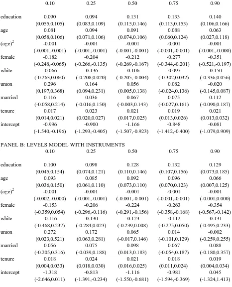
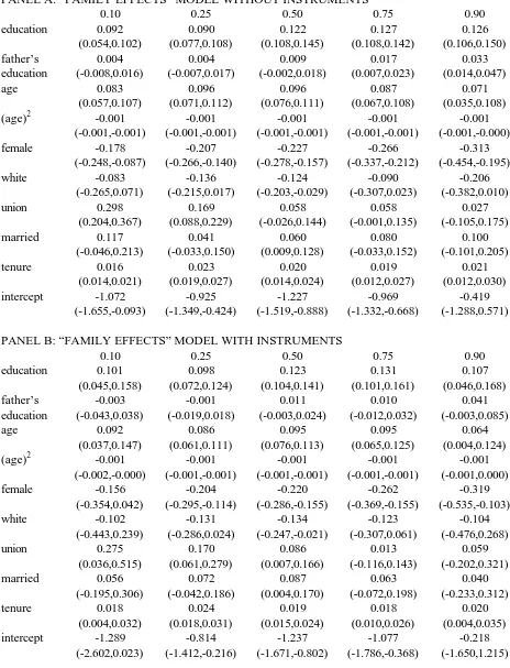
We finally briefly describe the return to the other covariates included in our empirical model.

Table 5 presents the returns to each of the variables for the “all” specification, which includes age,

race, gender (see Amidon, 1997), married, union, and tenure, along with the associated 90%

confidence intervals for the levels models.16 _{Table 6 does the same for the family effects models.}

Figure 6 is a concise summary of the results. It presents results for the family effects model without

IV. Note the anomalous negative effect of race on earnings which is also reported by Ashenfelter and

Krueger (1994) and Ashenfelter and Rouse (1998), but that this cannot be estimated with precision at

any quantile. The effect of marital status on earnings is positive but it is only significant at the median.

The other three sets of results in the two tables are very similar to the findings depicted in Figure 6.

For most of the covariates, there is little heterogeneity in the returns, except for the female and

union variables. Women in this sample earn about 18 percent less than men at low quantiles (0.1) but

the gap widens to roughly 30 percent at higher quantiles (0.9). The returns to being covered by a

union contract are also monotonically declining. At low quantiles (0.1) the return to being unionized is

roughly 0.3 and at upper quantiles the return is roughly zero. This last result is consistent with the

recent work that explores the effect of unions on the structure and the change in the distribution of

wages (DiNardo and Lemieux, 1996; DiNardo, Fortin and Lemieux, 1996).

5. Concluding Comments

In this paper we present estimates of a simple model of earnings and schooling choices in

which we explore the relationship between education and ability in the generation of human capital

without imposing a stringent parametric structure on this relationship. We use instrumental variables

quantile regression and data on identical twins to isolate the causal link between education and

earnings at different quantiles of the conditional distribution of wages, while dealing with potential

biases that arise from the correlation between ability and schooling investment choices and the fact

that observed education levels are imperfect measures of schooling.

The results suggest the existence of an important upward ability bias at the high quantiles in

the estimates of the returns to education that do not account for the endogeneity of schooling choices.

Nevertheless, the estimated returns to education accounting for the endogeneity of schooling are

positive and significant consistent with the human capital model in which education enhances earnings

potential. The results also suggest that the measurement error in schooling levels induces slight

downward biases in the estimated returns to education in the low quantiles that are intensified by

attempts to deal with the ability bias.

More importantly, the results provide novel evidence of the existence of two sources of

heterogeneity in the returns to education. First, there is some evidence of a differential heterogeneity

effect by which more able individuals become more educated. The resulting endogeneity biases appear

as apparent higher returns to education at the high quantiles. That is high-ability individuals appear to

have higher returns to schooling. Therefore, the earlier estimates of heterogeneous returns to schooling

from quantile wage regressions that do not control for unobserved ability (Buchinsky (1994) and

Mwabu and Schultz (1996)) may be confounding this differential endogeneity bias with any actual

within quantile difference in the marginal returns to education.

Second, once this endogeneity bias is accounted for, our results provide significant evidence

that there is no unique causal effect of schooling and that for any particular individual the effect may

be above or below the extensively documented OLS estimate depending on his or her unobservable

abilities in the generation of earnings. In particular, the evidence supports the existence of a

complementary relationship between ability and education which gives an advantage to those at the top

of the conditional wage distribution but also enhances earnings potential for low-wage individuals. The

results thus suggest that more able individuals may attain more schooling because of lower marginal

costs and due to higher marginal benefits to each additional year of education.

These findings are at odds with the findings of Ashenfelter and Rouse (1998) of lower

marginal returns for higher ability individuals after controlling for the endogeneity and measurement

error in schooling, but are consistent with recent findings of Conneely and Uusitalo (1998) based on

estimation of conditional mean wage functions. They are also consistent with Card’s (1995a)

proposition of a negative relationship between the marginal costs and the marginal returns to schooling

along the distribution of abilities.

Our results thus reassure us that any formal structural model of schooling investments and

earnings should allow for potential heterogeneity in the returns to education (Card, 1995a) and perhaps

diverse changes over time at different points in the wage distribution (Buchinsky, 1994, Chay and Lee,

1996).

There are several ways in which our work can be extended. First, a readily available extension

is a careful exploration of potential differential effects of observable individual characteristics such as

union participation and gender in the returns to education across quantiles of wage residuals. We

intend to do this in subsequent work. Second, it would be interesting to explore potential non-linearities

in the relationship between schooling and log-earnings by allowing the returns to education to differ

across different education levels as in Buchinsky (1994) and Mwabu and Schultz (1996). Third, one

could try to explore the impact that the changes over time in quantile estimates of the returns to

education have on the structure of wages and widening wage inequality while carefully addressing the

endogeneity and measurement error biases which are likely to change over time. This last point faces

data limitations and some challenging but interesting unsolved methodological problems, particularly

exploring extensions of quantile regression methods to the analysis of panel data.

In a recent paper, Bound and Solon (1998) criticized the estimates of returns to education

based on twins data questioning the assumption of independence between the earnings and optimal

education choice disturbances. As they rightly argued, the validity of twins based estimates relies

crucially on this assumption. In our final approach, the resulting estimated returns are never lower than

9 percent and can be as high as 13 percent at the top of the conditional distribution of wages. In the

case of failure of this assumption, our estimates can be thought to provide rather tight bounds on the

causal effect of education on earnings.

Finally, the existence of the two sources of heterogeneity suggests that typical estimates of the

mean return to education based on OLS provide a rather incomplete characterization of the impact of

education on labor market outcomes and are thus a poor guide for public policy. On the one hand, the

differential endogeneity bias that arises because of ability-based differences in the marginal costs of

education imply that there is room for policies aimed at promoting heavier schooling investment by

individuals who face higher costs. On the other hand, the indication that apart from this differential

ability bias, the returns to schooling are higher for those at the top of the conditional wage distribution

suggests a limit on the extent to which schooling can compensate for differences in individual ability

endowments. Even though a general educational policy will tend to increase the welfare of individuals

in the society, its net impact on the long run distribution of incomes and wealth will depend on the initial

References

Amidon, Carole, 1997, “Are Female Wage Earners Experiencing Wage Discrimination: An Application of Quantile Regression,” University of Illinois at Urbana-Champaign, June.

Angrist, Joshua, D., and Alan B. Krueger, 1991, “Does Compulsory Schooling Affect Schooling and Earnings?” Quarterly Journal of Economics, 196, November, pp. 979-1014.

Angrist, Joshua, D., and Alan B. Krueger, 1992 “Estimating the Payoff to Schooling Using the Vietnam-Era Draft Lottery,” National Bureau of Economic Research Working Paper: 4067, May.

Angrist, Joshua, D., and Whitney Newey, 1991, “Over-Identification Tests in Earnings Functions with Fixed Effects,” Journal of Business and Economic Statistics, 9, July, pp. 317-23.

Ashenfelter, Orley, and Alan Krueger, 1994, “Estimates of the Returns to Schooling from a New Sample of Twins,” American Economic Review, December, 84 (5), pp. 1157-1173.

Ashenfelter, Orley, and Cecilia Rouse, 1998, “Income, Schooling, and Ability: Evidence From a New Sample of Identical Twins,” Quarterly Journal of Economics, 113(1), February, pp. 253-84.

Becker, Gary, 1967, Human Capital and the Personal Distribution of Income. Ann Arbor, University of Michigan Press.

Bound, John and G. Solon, 1998, “Double Trouble: On The Value of Twins-Based Estimation of the Return to Schooling,” National Bureau of Economic Research, Working Paper 6721.

Buchinsky, Moshe, 1994, “Changes in the U.S. Wage Structure 1963-1987: An Application of Quantile Regression,” Econometrica, March, 62 (2), pp. 405-58.

Buchinsky, Moshe, 1995, “Estimating the Asymptotic Covariance Matrix for Quantile Regression Models: A Montecarlo Study,” Journal of Econometrics, 68 , pp. 303-338.

Butcher, Kristin F., and Anne Case, 1994, “The Effect of Sibling Composition on Women’s Education and Earnings,” Quarterly Journal of Economics, 109, August, pp. 531-564.

Card, David, 1995a, “Earnings, Schooling and Ability Revisited,” Research in Labor Economics, Solomon Polachek ed., JAI Press, Volume 14, pp. 23-48.

Card, David, 1995b, “Using Geographic Variation in College Proximity to Estimate the Return to Schooling,” in L. Christofides, E. Grant, and R. Swidinsky, editors, Aspects of Labour Market Behaviour: Essays in Honor of John Vanderkamp, University of Toronto Press, pp. 201-22.

Chay, Kenneth, and David Lee, 1996, “Changes in Relative Wages in the 1980s: Returns to Observed and Unobserved Skills and Black-White Wage Differentials,” Princeton University Industrial Relations Section Working Paper #372.