ARCIMBOLDO, a supercomputing method for crystallographic ab initio protein structure solution below atomic resolution

(1)

DOCTORAL THESIS

Title: ARCIMBOLDO, a supercomputing method for crystallographic ab initio

protein structure solution below atomic resolution.

Presented by: Dayté Dayana Rodríguez Martínez

Centre: IQS School of Engineering

Department: Bioengineering

Directed by: Prof. Dr. Isabel Usón Finkenzeller

C

.I

.F

. G

: 59069740 U

ni

ve

rs

it

at

R

am

on L

ul

l F

undac

ió P

ri

vada.

R

gt

re

. F

und.

G

ene

ral

it

at

de

C

at

al

uny

a núm

. 472 (

28

-02

-90)

C. Claravall, 1-3 08022 Barcelona Tel. 936 022 200 Fax 936 022 249

E-mail

(2)

TESIS DOCTORAL

Título: ARCIMBOLDO, un método de supercomputación para la determinación cristalográfica ab initio de estructuras de proteínas con resolución inferior a la atómica.

Realizada por Dayté Dayana Rodríguez Martínez

en el Centro: IQS Escuela de Ingeniería

y en el Departamento: Bioingeniería

Dirigida por: Prof. Dr. Isabel Usón Finkenzeller

C

.I

.F

. G

: 59069740 U

ni

ve

rs

it

at

R

am

on L

ul

l F

undac

ió P

ri

vada.

R

gt

re

. F

und.

G

ene

ral

it

at

de

C

at

al

uny

a núm

. 472 (

28

-02

-90)

C. Claravall, 1-3

08022 Barcelona Tel. 936 022 200 Fax 936 022 249

E-mail

(3)

TESI DOCTORAL

Títol: ARCIMBOLDO, un mètode de supercomputaciò per a la determinaciò cristal·logràfica ab initio d’estructures de proteïnes amb resoluciò inferior a l’atòmica.

Realitzada per : Dayté Dayana Rodríguez Martínez

en el Centre: IQS Escola d'Enginyeria

i en el Departament: Bioenginyeria

Dirigida per Prof. Dr. Isabel Usón Finkenzeller

C

.I

.F

. G

: 59069740 U

ni

ve

rs

it

at

R

am

on L

ul

l F

undac

ió P

ri

vada.

R

gt

re

. F

und.

G

ene

ral

it

at

de

C

at

al

uny

a núm

. 472 (

28

-02

-90)

C. Claravall, 1-3

08022 Barcelona Tel. 936 022 200 Fax 936 022 249

E-mail

(4)

List of Figures 3

List of Tables 5

Abbreviations 6

1 Introduction 8

1.1 The phase problem . . . 8

1.1.1 Current methods to overcome the phase problem . . . 8

1.2 Computational scenario . . . 15

1.2.1 Grid computing/Supercomputing . . . 15

1.2.2 Middleware . . . 17

1.2.3 Cloud computing . . . 18

1.3 The ARCIMBOLDO approach to solve the phase problem . . . 19

2 Goal Settings 22 3 Materials and Methods 24 3.1 Phaser . . . 24

3.1.1 Rotation . . . 26

3.1.2 Translation . . . 28

3.1.3 Packing . . . 28

3.1.4 Re-scoring . . . 29

3.1.5 Refinement and Phasing . . . 30

3.2 SHELXE . . . 30

3.3 HTCondor . . . 32

4 Results and discussion 37 4.1 ARCIMBOLDO: the central hypotheses underlying the method . . 37

4.1.1 Underlying algorithms . . . 41

4.1.2 Solution of test cases. . . 46

4.1.2.1 CopG, on the border of atomic resolution. . . 47 4.1.2.2 Glutaredoxin, as a test for anα-β structure at 1.45˚A 49 4.1.2.3 Glucose isomerase, a TIM barrel protein at 1.54˚A . 49

(5)

4.1.2.4 EIF5, solution of a mainly helical, 179 amino acids

protein at 1.7˚A . . . 51

4.1.3 Extension to incorporate stereochemical information into ARCIMBOLDO . . . 52

4.1.4 Extension to incorporate complementary experimental in-formation into ARCIMBOLDO . . . 56

4.1.5 Practical use of ARCIMBOLDO and tutorial . . . 58

4.1.5.1 Preliminary considerations . . . 59

4.1.5.2 Setup for general variables . . . 60

4.1.6 Ab initiocase results on the first new structure phased, 3GHW. 62 4.1.6.1 Input files . . . 62

4.1.6.2 Data analysis . . . 63

4.1.6.3 Definition of variables for ARCIMBOLDO/Phaser 65 4.1.6.4 Density modification with SHELXE . . . 72

4.1.6.5 Lauching ARCIMBOLDO and checking results . . 74

4.1.6.6 ARCIMBOLDO folder structure . . . 75

4.1.6.7 MR folder structure and its input/output files . . . 77

4.1.6.8 Density modification folder structure and input/out-put files . . . 85

4.1.7 Libraries of alternative model-fragments case tutorial . . . . 86

4.1.7.1 Data analysis . . . 87

4.1.7.2 Definition of variables for ARCIMBOLDO/Phaser 88 4.1.7.3 Density modification with SHELXE . . . 93

4.1.7.4 ARCIMBOLDO folder structure . . . 94

4.1.7.5 MR folder structure and input/output files . . . 94

4.1.7.6 Density modification folder structure and input/out-put files . . . 94

4.2 Macromolecular structures solved with ARCIMBOLDO . . . 95

5 Summary and Conclusions 103

A Scientific production 105

B Posters presentations 107

(6)

1.1 Dual Space recycling algorithm . . . 13

1.2 Charge flipping algorithm . . . 14

1.3 Grid layers . . . 16

1.4 Grid task management . . . 18

1.5 Cloud actors . . . 19

3.1 Euler angles representing rotations . . . 26

3.2 Example of an HTCondor grid . . . 34

3.3 HTCondor matchmaking. . . 34

4.1 Rudolf II painted by G. Arcimboldo as Vertumnus . . . 40

4.2 Molecular chirality . . . 40

4.3 Small model producing several correct solutions . . . 40

4.4 Locating the 1st model . . . 42

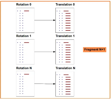
4.5 Rotation search of N+1 model . . . 43

4.6 Translation search of N+1 model . . . 43

4.7 Translation average prune . . . 44

4.8 Solutions selection by cutoff . . . 44

4.9 Packaging input files . . . 45

4.10 CopG solution . . . 47

4.11 Sheldrick’s rule: dependency of direct methods on atomic resolution 48 4.12 GI solution . . . 50

4.13 EIF5 solution . . . 51

4.14 LLG Rotation test for alternative models . . . 54

4.15 Z-score Rotation test for alternative models . . . 54

4.16 PRD2 superposed to models with side-chains . . . 56

4.17 VTA solution by locating anomalous substructure . . . 57

4.18 Schematic flow of the ARCIMBOLDO procedure . . . 58

4.19 Scalars, arrays and hashes . . . 60

4.20 ARCIMBOLDO ab initio path . . . 62

4.21 PRD2 crystallographic structure . . . 63

4.22 XPREP output of ISIGMA for PRD2. . . 64

4.23 PRD2 XPREP analysis of intensities statistics . . . 64

4.24 F and SIGF labels . . . 65

4.25 Linked search-parameters . . . 67

4.26 PRD2 Linked search-parameters . . . 67

(7)

4.27 Checking CC values . . . 74

4.28 Files and folders of ab initio solution . . . 75

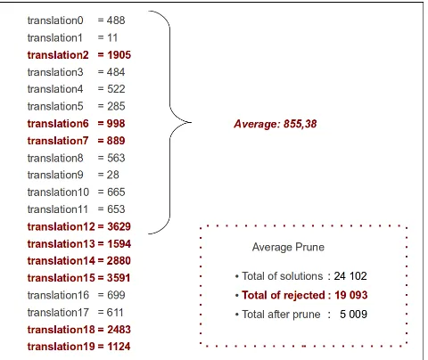
4.29 Translation files pruning with average I . . . 76

4.30 Translation files pruning with average II . . . 77

4.31 3 sets of 3 helices that solve PRD2 . . . 85

4.32 ARCIMBOLDO Alternative model-fragments path . . . 86

4.33 Hecke’s structure solution with superposed models . . . 97

4.34 Endless polymeric chains in the P61 crystals . . . 97

4.35 Structure of a Coiled Coil at 2.1˚A from the group of Mayans . . . . 99

(8)

3.1 Indication of a structure being solved through the TFZ-score values 26

3.2 Common SHELXE options within ARCIMBOLDO . . . 32

3.3 Example of ClassAds matching . . . 35

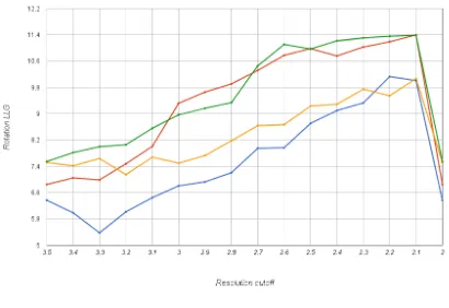
4.1 Resolution cutoff tests with CopG . . . 48

4.2 Previously unknown structures solved with ARCIMBOLDO . . . . 95

4.3 Analysis of CMI Phaser and SHELXE results . . . 101 4.4 Analysis of CMI top 10 Phaser results . . . 101

(9)

aa aminoacid

AU AsymmetricUnit

CC Correlation Coefficient

CPU Central Processing Unit

FCSCL Fundación Centro de Supercomputación de Castilla y León

FOM Figures Of Merit

HTC High Throughput Computing

IP Infrastructure Provider

MAD Multi-wavelength Anomalous Dispersion

MIR Multiple Isomorphous Replacement

MIRAS Multiple Isomorphous Replacement plusAnomalous Scattering

MPE Mean Phase Error

MR MolecularReplacement

NFS Network File System

NIS Network Information System

NMR NuclearMagnetic Resonance

PDB ProteinData Bank

RaaS Results asa Service

RIP Radiation damage Induced Phasing

rmsd root mean square deviation

SP Service Provider

SU Service User

SAD Single-wavelength Anomalous Dispersion

SIR Single Isomorphous Replacement

SIRAS Single Isomorphous Replacement plus Anomalous Scattering

VO Virtual Organization

VRE Virtual Research Environment

(10)

(11)

Introduction

1.1 The phase problem

Crystallography is arguably the most powerful of all structural techniques. Through the determination of the electron density map, it is able to deliver an accurate three-dimensional view of the biomacromolecular structures. Albeit, in order to calculate electron densities

ρ(xyz) = 1

V

X

h

X

k

X

l

|F(hkl)|

| {z }

Amplitudes

cos 2Π(hx+ky+lz−φ(hkl) | {z }

P hases

)

both magnitudes and phases of the x-ray diffraction maxima are required, but only the intensities are available from the diffraction experiment, hence, the density function cannot be calculate without retrieving the phases. This fundamental problem in crystallography is also known as the crystallographic phase problem[1]_.

1.1.1 Current methods to overcome the phase problem

In the case of small molecules -that is for chemical crystallography- the phase problem can usually be solved directly. In protein crystals diffraction is limited by their intrinsic nature while the number of variables required to determine the structure is much larger. The term resolution refers to the maximum resolution to which a macromolecular crystal diffracts, that is the minimum spacing between parallel planes of atoms from which diffraction can still be recorded. More closely spaced planes lead to reflections further from the center of the diffraction pattern. In the present work, atomic resolution will be used to design data collected to 1.2˚A or beyond, high resolution to data of 2˚A or better: the resolution to which 50% of the crystal structures deposited with the Protein Data Bank[2,3] _diffracts.

The mathematical complexity of the problem rules out an analytical solution, and it has to be reduced in order to establish a rough initial electron density map or model, what is known as phasing. In macromolecular crystallography there are

(12)

several methodologies to retrieve the missing phases involving both experimental and computational methods:

Experimental Phasing

It is based on using substructures of anomalous scatterers or heavy atoms, to provide reference phases for the full structure to be determined. Crystals can be modified to incorporate heavier elements,[4,5] _{so that differences induced}

by their presence can be determined. For crystals containing -or derivatized to contain- anomalous scatterers, diffraction data can be recorded at wave-lengths selected to affect the scattering behaviour of this particular element. Max Perutz[6] and John Kendrew[7] were the first to exploit the presence of heavy atoms in proteins for phasing. To introduce the heavy atoms into the crystals, they can be soaked in a heavy atom solution. Alternatively, the pro-tein can be derivatized previously to crystallization or crystallization can be accomplished in the presence of the heavy atom. Ideally, the heavy atoms occupy ordered positions within the crystal, as their affinity to particular chemical environments drives their association to the protein, while only minimally disrupting the three-dimensional structure of the protein, that is native and derivative crystals are isomorphous, keeping the native crystal spacegroup and unit cell dimensions within a small percentage. Heavy atoms contribute significantly to the diffraction, making their contribution easy to detect. The difference of the diffraction pattern of the derivative and native crystals can be used to determine the positions of the heavy atoms. With di-rect, Patterson or dual-space recycling methods (see below) the heavy atom substructure can be solved.

This approach to phasing is called Single Isomorphous Replacement

(SIR), the trigonometric relationships involving the phases and structure factors of native, derivative and substructure are fulfilled by two possible phase values. Thus, the problem is underdetermined since the number of variables is larger than the available equations, therefore, further experimen-tal information or constraints must be applied in order to solve the structure. By using at least one other heavy atom derivative the phase ambiguity can

be solved, this method is called Multiple Isomorphous Replacement

(MIR). The attempts to get a proper derivative could be unsuccessful for lack of specific binding, insufficient derivatization or lack of isomorphism, along with other error sources. In addition, these derivative data are usually discarded once the target structure is solved, which together with the fact that the number of experiments that must be carried out to find a good sub-structure is unpredictable, poses an impractical increase in the time scale, resource needs and experimental effort of the crystallographic study.

The lack of isomorphism issue can be solved by recording anomalous data at various wavelengths on the same crystal as long as radiation damage[8] _does

not prevent it. Macromolecules, being chiral by nature, invariably crystal-lize in one of the 65 chiral, and thus acentric spacegroups. In the presence of anomalous scatterers, at appropriate wavelengths, Friedel’s Law breaks down in acentric spacegroups. It states that the intensities of the h, k, l

(13)

of Friedel’s Law is that even if the space group lacks a center of symmetry, the diffraction pattern is centrosymmetric and it is not possible to tell by diffraction whether an inversion center is present or not.

The reason for Friedel’s rule is that, according to the geometrical theory of diffraction, the diffracted intensity is proportional to the square of the modulus of the structure factor|Fh|2. The structure factor is given by

Fh =P_jfjexp(−2πih.rj)

where fj is the atomic scattering factor of atom j, h the reflection vector

and rj the position vector of atom j. If the atomic scattering factor, fj, is

real, the intensities of theh,k,l and-h,-k,-l reflections are equal, it follows:

|Fh|2 =FhFh∗ =FhF¯_h =|F¯_h|2

However, if the crystal is absorbing due to anomalous dispersion, the atomic scattering factor is complex andd

F¯_h 6=F_h∗

The anomalous dispersion corrections take into account the effect of absorp-tion in the scattering. The total scattering factor of an atom is a combinaabsorp-tion of different contributions, and at particular wavelength ranges the absorption effect is large enough to be exploited:

f(λ) =fo₊_f0₍_λ_{) +}_if00₍_λ₎

fo_{, the normal scattering factor -which is independent of the}

wavelength-and f0 and f00, the anomalous scattering factors -which account for real and imaginary components- that change with the wavelength. For X-ray energy values where resonance exists, f0 usually decreases dramatically the real scattering component, while the value of the imaginary component f00

is positive[9].

If the anomalous signal is recorded at a single wavelength value, the phas-ing procedure is called Single-wavelength Anomalous Dispersion[10,11]

(SAD), if otherwise the anomalous signal is detected at different wavelength values, it is calledMultiple-wavelength Anomalous Dispersion[12]_(MAD).

(14)

Many recombinant proteins can be obtained in prokaryotic expression sys-tems while replacing methionine residues by selenium-methionine[14]. Se-lenium is an appropriate anomalous scatterer as its absorption edge corre-sponds to a wavelength that is readily accessible at synchrotron beamlines. Radiation damage[15] induces errors that might hinder the determination of reliable differences within the anomalous experiment. It is present even in crystals held at cryogenic temperatures (100K), the longer the crystal is exposed to X-ray radiation the higher the effect of the radiation damage increasing the amorphous or disordered volume of the crystal sample. The underlying cause of this damage is that the energy lost by the beam in the crystal -owing to either the total absorption, or the inelastic scattering of a fraction of the X-rays as they pass through the crystal- induces physical changes and chemical reactions in the sample.

MIRAS/SIRAS are experimental phasing techniques developed to solve crys-tallographic structures by combining isomorphous replacement and anoma-lous dispersion. This combination leads to an overdetermined problem by introducing more equations. Anomalous signal can be obtained from heavy atoms at suitable wavelengths, therefore single/multiple isomorphous re-placement with anomalous signal scattering is powerful combining the strength of both methods if the appropriate experimental setup is available.

Finding the position of the heavy atoms and/or anomalous scatterers can be used to provide reference phases[16] _{for the structure to be solved. This}

has a comparable effect to introducing or differentiating a small molecule structure within the target macromolecule, which can be effectively solved by Patterson or direct methods. If the coordinates of the substructure can be obtained, phases for the whole structure can be derived and a starting model can be built[17,18] into the resulting electron density map.

Molecular Replacement

Relies upon knowledge from a previously solved similar structure to provide the missing phases and takes a different approach: locating a large number of lighter atoms (at least, most of the main-chain) as a rigid group[19]_{. It is}

based on the fact that macromolecules of similar sequence tend to have very similar structures by conserving their folds[20].

Possible orientations and positions of the solved model are tried in the unit cell of the unknown crystal[21] until the predicted diffraction best matches the observed ones aided by the Patterson function or Maximum-likelihood methods[22]_{. Then the unknown phases are estimated from the phases of the}

known model and an initial map is calculated with the ”borrowed” phases and the observed amplitudes which are going to contribute in the rebuild-ing/refinement process supplying the information that will make the model closest to the target.

This approach becomes more powerful as the available structural knowledge deposited in the Protein Data Bank[2,3] _{grows larger. It is fast, efficient}

(15)

and consequently, especially at low resolution, the calculated structure may be biased towards the phasing model.

The above mentioned methods are general methodologies that involve automated computational techniques at the final steps of their schedules, but, to achieve phasing, they all depend on experimental and/or particular, theoretical starting information at the initial stage of their layouts.

Methodologies demanding less initial experimental effort or particular structural knowledge, and thus more shifted to automated computational techniques would constitute a clear advantage. In this scenario, general ab initio methods, able to solve biomacromolecules using only a native dataset of amplitudes, without the use of a previously known related structure or phase information from isomorphous heavy atoms or anomalous scatterer derivatives would be desirable. Pureab initio

methods may not involve specific structural information, however, general features that are not specic to the structure in question can be utilized[23]_.

The ab initio field involves several approaches:

Patterson: the convolution of the electron density with itself can be calculated

through the Fourier transform of the experimentally measured diffraction inten-sities[24]_{. This function does not contain phase information, but it has valuable}

information about interatomic vectors that can be used to determine their rel-ative positions. The height of the maxima are proportional to the number of electrons of the atoms involved. Once a Patterson map is available, a correct interpretation may allow to get the absolute position of some atoms and use them to find the rest. This is feasible for heavy atoms within small molecules but does not scale well for macromolecules as the peaks originated from indi-vidual pairs of atoms are less prominent and heavily overlapped. Nevertheless, using its interpretation to aid other sophisticated techniques has been crucial in the solution of complex problems[25]_.

Direct methods: the unmeasured phases are not independent and

relation-ships among them can be drawn for a particular set of measured intensities, based on probability theory derived from the application of nonnegativity and atomicity constraints[26]_. _{This method exploits the fact that the}

crystallo-graphic problem is heavily overdetermined at atomic resolution, which means that there are many more measured intensities than parameters that are nec-essary to describe an atomic model and therefore, it requires high resolution datasets. It is generally effective in the solution of small molecules up to 200 atoms[27] _{and has been widely used and implemented in crystallographic}

com-puter programs giving birth to a new generation of methods based on direct methods:

Dual space recycling: currently, recycling between real and reciprocal

(16)

While classical direct methods, in their original form, work entirely in re-ciprocal space, dual space recycling switches back and forth between real and reciprocal spaces to effectively enforce the atomicity constraint in both formalisms. This approach has come to be known as Shake and Bake[28,29]

[image:16.596.128.519.199.373.2]

and consists on alternate trials of local minimization technique to be applied in reciprocal space (Shaking) with atomicity and nonnegativity constraints explicitly imposed in real space (Baking).

Figure 1.1: Dual Space recycling algorithm[23,30]_.

It still depends on high resolution information, yet successful on extending the power of direct methods into the scope of small macromolecules (≈1,000 equal atoms[23] _{and 2,000 atoms for structure containing heavy atoms}[31]_).

Charge flipping: a member of the dual space recycling family. It follows an

iterative Fourier cycle that unconditionally modifies the calculated electron density and structure factors in dual spaces. The real-space modification simply changes the sign of the charge density below a threshold, which is the only parameter of the algorithm. Changing the sign of electron density be-low a small positive threshold simultaneously forces positivity, and introduces high-frequency perturbations to avoid getting stuck in a false minimum. In reciprocal space, observed moduli are constrained using the unweighed ob-served amplitudes (Fobs) map, while the total charge is allowed to change freely[32,33]_.

(17)

Figure 1.2: Charge flipping algorithm.

1. %(r) → g(r): Real-space modification of the electron-density map, ob-tained by flipping the low-density region.

2. g(r)→G(q): Fourier transform to reciprocal space.

3. G(q) → H(q): Reciprocal-space modification of calculated structure factors, in practice replaced by the observed amplitudes.

4. F(q)→%(r): Inverse Fourier transform to real space.

The method is able to solve large structures and even proteins if high reso-lution data are available and a couple of heavy atoms (calcium or heavier) are present[34]_.

VLD: is named after vive la difference and allows the recovery of the cor-rect structure starting from a random model through cyclic combinations of the electron densities of the random selected model and the expected ideal difference Fourier synthesis[35].

Once a random model has been selected, the difference electron density should provide a map well correlated with the ideal one. Suitably mod-ified and combined with the electron density of the model, it should de-fine a new electron density no longer completely random, which, rede-fined by electron-density modification to meet its expected properties (e.g. positivity, atomicity, solvent properties etc.) may lead to a better structural model. Roughly speaking, the difference electron density provides a difference model, which is refined via cycles of density modification. The method is able to solve medium-size molecules and proteins of up to 9,000 atoms containing heavy atoms[31]_{, provided the data have high, though not necessarily atomic}

resolution.

(18)

1.2 Computational scenario

Given that the crystal structures of the first macromolecules were determined over 50 years ago[6,7,36], crystallography has started exploiting computing almost from its cradle. This has motivated a highly efficient use of resources in the evolution of crystallographic software. Methods programmed to run on computing centres 40-30 years ago were highly efficient, fast enough to be transferred to run on personal computers with risk, pentium or xeon processors. Thus, a scientific community regularly using computing, has largely turned its back on supercomputing. Still, the use of massive calculations allows to solve problems in completely different ways as algorithms -that would be prohibitive on a desktop machine- become amenable. The advantage is not to calculate the same faster, but rather to enable a different approach.

1.2.1 Grid computing/Supercomputing

Supercomputers are an extremely powerful type of computing systems (hardware, systems software and applications software) the most powerful available at a given time. They are composed by a large number of CPUs often functioning in parallel, actually, most of them are really multiple computers that perform parallel pro-cessing. Supercomputers have huge storage capacity and very fast input/output capability, but they are very expensive and so primarily used for scientific and engineering work[37]_.

In the absence of a supercomputer or just to optimize the project budget, high performance/throughput computing can be performed in networked frameworks as long as it is possible to divide the main goal into smaller and individual tasks. Grid computing can arise as an attainable alternative to supercomputers for solv-ing scientific problems, backed up by strong reasons as cost reductions and resource availability.

A computing grid is a distributed system that supports a virtual research envi-ronment (VRE) across different virtual organizations[38] _{(VO), it well encases the}

collaborative work in the scientific world as sharing large volume of data among research groups is the norm.

A virtual organization merge in a set of individuals and/or institutions defined by sharing rules. The VOs can vary in purpose, scope, size, duration, structure, etc., but they all concern about highly flexible sharing relationships and sophisticated and precise levels of control over how shared resources are used[39]_.

This distributed infrastructure offers a useful tool to fulfil the needs of each client by squeezing the hardware capabilities of geographically dispersed resources, bring-ing together different operative systems and hardware platforms whose perfor-mance is higher on average, creating a virtual supercomputer which has the ca-pacity to execute the tasks that, otherwise, would not be achievable by its single part-machines apart.

(19)

affordable by way of parallel computing. Grid-computing environment better suits organizations that are already used to high performance/throughput computing or somehow oriented to distributed computing. A grid computing system comes together with administration and accounting resources issues being as it involves multiple members, which requires proportionality between their contributions. The grid technology offers protocols, services and tools that accomplish the men-tioned requirements by means of:

• Security solutions.

• Resource management and monitoring protocols and services.

• Data management services that locate and transport datasets between stor-age systems and applications.

[image:19.596.123.523.363.612.2]

The model of a computing grid enables the availability of an efficient network infrastructure, larger computing power and additional hardware for the different-constituent VOs. It can be described by its components as a layer-based structure:

Figure 1.3: Layered structure of grids[38]_.

(20)

needs of the various VOs within a VRE, that uses the services of the management software layer. Any user-specific application forms the top layer and only accesses the services of the discipline-specific software layer[38].

1.2.2 Middleware

In the field of computing systems, a job is the unit of work given to the operating system, e.g., a job could be the run of an application program, and it is usually executed without further user intervention. A similar term is task, that can also be applied to interactive work.

Middleware software is key for the optimal functioning of a grid computing system, its role within the management software layer is to connect the different parts of the grid while offering at least elementary services such as job execution, security, information and file transferring. However, it may offer as well more advanced services including file, task and information management. Middleware software should hide the underlying complexity of the grid as much as possible, but should provide enough flexibility that individual control about a file transfer can be is-sued[40]_.

The job execution services must be able to submit a job and to check its

sta-tus at a any given time. Jobs must have a unique identifier so that they can be properly distinguished.

Security services should involve authentication and authorization to protect

re-sources and data on the grid. Because of the large number of rere-sources in the grid, it is important to establish policies and technologies that allow the users to sign-on through a single interaction with the Grid.

Information services provide the ability to query for information about

re-sources and participating services on the grid and must be able to deal with the diverse nature of queries directed to it.

File transfer services must be available to move files from one location to

an-other sophisticatedly enough to allow access to high-performance and high-end mass storage systems. Often such systems are coupled with each other and it should be possible to utilize their special capabilities in order to move files be-tween each other under performance considerations.

(21)

[image:21.596.120.517.86.343.2]

Figure 1.4: Complexity of Grid task management[40]_.

There are several approaches of grid computing software now available: HTCon-dor[41], ARC[42], Globus[43], UNICORE[44], etc. Each one is unique because the interpretation of protocols and standards can vary significantly as well as the un-derlying platforms.

1.2.3 Cloud computing

Nowadays, computing is transforming from applications running in individual com-puters to services demanded by users from anywhere in the world, offering results based on the user requirements and served without regard to where they are hosted or how they are delivered. Clouds are promising to provide services to users with-out reference to the infrastructure on which they are hosted.

A Cloud is a type of parallel and distributed system consisting of a collection of interconnected and virtualized computers that are dynamically provisioned and presented as one or more computing resources based on service-level agreements established through negotiations between the service provider and consumers[45]. It presents the opportunity to reduce or eliminate costs bound to in-house provi-sion of those services by making them available on demand and removing the need of heavy invests, plus difficulties in building and maintaining complex computing infrastructures.

The service providers make services accessible to the service users through

web-based interfaces. Clouds aim to outsource the provision of the computing in-frastructure required to host services. This inin-frastructure is offered ”as a service”

by infrastructure providers, moving computing resources from the SPs to the

(22)

[image:22.596.114.518.87.329.2]

Figure 1.5: Cloud actors[46].

It is a new way of providing and utilizing resources, but by no means should be considered a competitor to grid-computing technology as both approaches can benefit from each other[38]_.

1.3 The ARCIMBOLDO approach to solve the

phase problem

ARCIMBOLDO materializes a new approach to render macromolecular ab initio

phasing generally successful, rather than limited to exceptional cases, through the exploitation of parallel computing. Its application has afforded the practical re-sults reflected in the publications attached.

The aim of this thesis is to lay out the development of the method in the course of the last years, which started by using molecular replacement (MR) to place small secondary structure models such as the ubiquitous main-chain helix against a native dataset of amplitudes, and to subject the resulting phases to a density modication and autotracing procedure in a supercomputing frame.

The algorithm is conceived as a multisolution method that generates many starting hypotheses, therefore it is controlled by sophisticated filters to limit the number of parallel jobs that have to be calculated within tractable limits and to discriminate successful solutions automatically through reliable figures of merit.

(23)

and many more indistinguishable, partial solutions have to be pursued, requiring a more powerful computational resources.

Nevertheless, the tasks to be executed are very easy to parallelize and suitable for a grid environment. The highly heterogeneous hardware and operative systems characterizing the limited computing resources we had access to at the beginning of our project, attracted our attention to an open-source high throughput product named HTCondor[47] _{that allows to run multiple instances of the same software,}

just slightly varying the input, on a large number of otherwise idle or sub-utilized processors, regardless of their heterogeneity.

A condor-grid was then configured and exploited for our experiments at the In-stitute of Macromolecular Biology of Barcelona (IBMB in Spanish) and later a collaboration was established with the Foundation of Supercomputing Center of Castile and Le´on (FCSCL in Spanish). The condor-grid environment tested at IBMB was then exported to Calendula, a supercomputer with hardware charac-teristics compatible with our first experimental workspace.

Macromolecular crystallographic structures have always entailed a difficult com-puting problem to solve. This is originated by the existence of two important differences with small molecule crystals: size and resolution. Both of them hinder direct methods when applied to proteins and although they are generally effective for small molecules, methods based on probabilistic phase relations have been rel-egated to a small number of cases, notably large antibiotics, with characteristics closer to small molecules than to macromolecules that precluded the use of stan-dard protein methods[23]_.

Of the two barriers just mentioned, resolution is the most difficult to overcome. The available resolution determines the amount of information obtained from a given crystal form in the diffraction experiment, the total number of unique diffrac-tion intensities being higher, the higher the resoludiffrac-tion. The difference in resoludiffrac-tion will be reflected in the quality of the electron density map, a higher data resolu-tion comporting a higher level of detail in the electron density map, which in turn leads to higher accuracy of the positions of the atoms in the model determined. In the present work we have pursued the relaxation of resolution values. Protein or peptide structures of small size can not be solved by direct methods in the absence of atomic resolution. The size limitation for direct methods is well found in the mathematical background, and though size is a constant parameter for each structure, data resolution depends on the diffraction experiment and is thus con-ditioned by the crystallization procedure, the researcher skills, and the diffraction platform. Nevertheless, the possibilities to improve the diffraction properties of a given crystal form are limited as well by the intrinsic nature of the crystal. Not just the resolution limit, but also the completeness of the data is a main factor for ab initio methods to succeed, experiments have proved that even extrapolated values of non measured data improves the quality of the final electron-density map[48]_.

(24)

(25)

Goal Settings

Ab initio, direct methods[23], solve the phase problem through probability theory derived from the positivity of the electron density map and atomicity constraints. To be satisfied, these constraints require atomic resolution data and although they perform exceedingly well for small molecules, in the field of macromolecules their applicability is hindered by the requirement of exceptionally high resolution, fur-ther complicated by the large number of atoms to be located.

However, the fact that proteins are composed by building blocks of known geom-etry like α-helices and β-strands, which can be predicted from their amino acid sequence, provides a possible general alternative to atomicity, as a means of bring-ing in prior stereochemical information that can and must be used to extend the classical ab initio macromolecular phasing methods.

The main subject of this project has been the development of a new computational method of general applicability at medium resolution -around 2˚A- to overcome the phase problem relying only on a dataset of native diffraction amplitudes and with-out previous detailed structural knowledge or measurements of heavy atoms or anomalous scatterer derivatives.

We focused our attention in mainly helical macromolecular proteins given the ten-dency of α-helices to be more rigid in their main-chain geometry than β-strands, the almost ubiquitous presence ofα-helical main-chain fragments in protein struc-tures (78% of the strucstruc-tures deposited in the Protein Data Bank[2,3] _{contain this}

secondary structure element), and their predictability from the known amino acid sequence or even from data features such as the Patterson function or the Wilson plot even in the absence of sequence information.

The planned objectives for this thesis were:

• To achieve macromolecular ab initio phasing, using only a dataset of na-tive amplitudes and without detailed structure knowledge, measurements of heavy atoms or anomalous scatterer derivatives.

• To relax the previous stringent requirement for atomic resolution data, tar-geting a typical macromolecular resolution limit, fulfilled by half of the struc-tures deposited in the PDB: 2˚A.

(26)

• To combine the advantages of some of the currently available phasing meth-ods, integrating complementary sources of phase information into a new method of general applicability.

• To exploit grid and supercomputing resources in a multisolution frame, de-signing a parallel tasks environment in order to decrease the time cost.

• To develop the method testing it on already known macromolecular struc-tures.

• To solve previously unknown protein structures with resolution, size and composition beyond the scope of the aforementioned methods when inde-pendently working.

• To develop and optimize different branches of the method depending on the starting information available.

(27)

Materials and Methods

ARCIMBOLDO[53] _{is a methodology of general applicability for}

macromolecu-lar phasing at medium resolution, around 2˚A, which works in a multisolution frame by combining the correct location of accurate small model-fragments with the program Phaser[54] _{and density modication and autotracing with the program}

SHELXE[55]_{. Given its multisolution nature, it requires grid/supercomputing}

en-vironments.

3.1 Phaser

Phaser[54]is a widely used MR program that has been developed by Randy Read’s group at the Cambridge Institute for Medical Research (CIMR) in the University of Cambridge. It can be found associated to the CCP4[56] _{suite of programs for}

macromolecular structure determination as well as to PHENIX software suite[57]. MR in Phaser is based on maximum likelihood probability theory target func-tions[58]_{, to better take into account the incompleteness and inaccuracy of the}

search model. This suits well the case of small main-chain fragments, necessarily representing a very partial fraction of the correct structure.

Maximum likelihood states that the best model is most consistent with the ob-servations: experimental data and prior knowledge. Consistency is measured sta-tistically by the probability that the observations should have been made; if the model is changed to make the observations more probable, the likelihood goes up indicating that the model agrees better with the data. One way to think about likelihood is imagining that data have not been measured yet, a model is avail-able with various parameters to adjust (coordinates and B-factors in the case of crystallography), as well as some model concerning the sources of error and how they would propagate. This allows to calculate the probability of any possible set of measurements and to see how well they agree with the model.

Probability distributions in experimental science are often Gaussian, and then likelihood becomes equivalent to the least-squares formulation. In the case of crystallography, the (phased) structure factors have Gaussian distributions, but

(28)

the phase information is lost when intensities are measured, and the distributions of the measurements are no longer Gaussian. This is why it is necessary to go to first principles and apply likelihood.

The standard Phaser procedure possesses a high degree of automation, however, the step by step algorithm can be divided in convenient blocks ofrotation,

trans-lation, packing, re-scoring and refinement and phasing tasks, that can be

invoked using traditional CCP4 keyword-style input.

Each of these processes depends on specic input lines, some of which are common to all of them:

• Mandatory

– Phaser task to execute

– MTZ file containing observed data.

– Labels contained in the MTZ file and used for the structure factor amplitudes and their standard deviations.

– Model(s) in the form of a pdb file.

– Molecular weight of the protein.

– Number of molecules in the asymmetric unit (AU).

• Optional

– Potential solution(s) to be used.

The output files indicate the particular figure of merit (FOM) for every process each solution has passed through:

RFZ: Rotation Function Z-score.

TFZ: Translation Function Z-score.

PAK: Number of clashes in the packing.

LLG: Log-Likelihood-Gain.

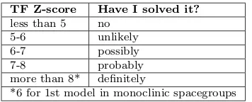
Signal-to-noise is judged using the Z-score, which is computed by comparing the LLG values from the rotation or translation search with LLG values for a set of random rotations or translations. The mean and the root mean square deviation (rmsd) from the mean are computed from the random set, then the Z-score for a search peak is defined as its LLG minus the mean, all divided by the rmsd, i.e.

the number of standard deviations above (or below) the mean.

(29)

TF Z-score Have I solved it? less than 5 no

5-6 unlikely 6-7 possibly 7-8 probably more than 8* definitely

[image:29.596.336.514.84.156.2]

*6 for 1st model in monoclinic spacegroups

Table 3.1: Indication of a structure being solved

through the TFZ-score values according to the Phaser manual.

For the translation function the correct so-lution will generally have a Z-score over 5 and be well separated from the rest of the solutions. The table provided in the Phaser manual gives a rough guide to in-terpreting TF Z-scores, these values are to be trusted in the conventional MR context, but very incomplete models represent a dif-ferent case, to be determined from system-atic molecular replacement trials.

When searching for multiple components, the signal may be low for the first few components but, as the model becomes more complete, the signal should become stronger. Finding a clear solution for a new component is a good sign that the partial solution to which that component was added was indeed correct. In our particular use scenario, the fragments to be located invariably constitute a very small fraction of the total structure, although they tend to be very accurate.

3.1.1 Rotation

The rotation task is performed to obtain the orientation of a model expressed in

α, β and γ Euler angles, the notation φ, θ, ψ is also frequently used.

Figure 3.1: Euler angles

representing rotations:xyz is the original frame, XYZ is the rotated one and the

intersection of xyandXYis represented byN.

To understand how a rotation is represented by such angles, let us define xyz as the axes of the original co-ordinate system, XYZ as the axes of the rotated one andNas the intersection of thexyandXY coordinate planes. Within this reference frame, α is the angle be-tween thex-axis and theN-axis,β is the angle between the z-axis and the Z-axis and γ is the angle between the N-axis and theX-axis[59].

The rotation likelihood function can be approximated through two different functions: the brute-force or fast rotation. In both cases a rotation function for the model is calculated on a grid of orientations covering the rota-tional asymmetric unit for the spacegroup of the crystal. The function used for a brute search[60] represent a bet-ter approximation to the likelihood target and is thus, very exhaustive and slow to compute, therefore recom-mended only when the space for the search can be restricted using additional information. The fast rotation function[61] _{represents a signicant speed}

improve-ment, at the price of calculating one term less.

In addition to the mandatory input parameters mentioned above, Phaser rotation searches also demand:

(30)

• Model to orient against diffraction data.

Its output is written to files with extensions.outand.rlist. The latter contains a condensed summary of the solutions produced in the run, exhaustively detailed in .out files. Files with extension .rlist contain the set(s) of orientations that best satisfy the chosen rotation function together with the observed data, sorted by a given FOM, and selected after applying a given cutoff, e.g:

SOLU SET

SOLU TRIAL ENSEMBLEensemble1EULER 138.693 77.189 91.309 RFZ 3.68

Each line contains the label associated to the oriented model (highlighted in bold) and the calculated values for α, β and γ Euler angles that will become the input for the translation search. At the end of the line, underlined, the value of the Rotation Function Z-score (rotation FOM) is expressed.

The example displayed corresponds to a set of solutions calculated for the 1st orientation search of a model, but, for subsequent fragments, a rotation can also be calculated once a model-fragment has been placed. This information might come from different sources, for example, additional knowledge concerning the position of a substructure or a previous solution that is not in itself enough to achieve successful phasing, but can contribute with partial information to a combined search. In such cases, the output file of potential orientations for the placement of a new model-fragment might look like this:

SOLU SET RFZ=2.9 TFZ=4.4 PAK=0 LLG=7 LLG=12 TFZ==0.5

SOLU 6DIM ENSE ensemble1 EULER 134.873 78.270 219.973 FRAC 0.49572 0.54601 0.96696 BFAC -3.32103

SOLU TRIAL ENSEMBLE ensemble1 EULER 141.203 81.674 91.277RFZ 3.53

The FOMs underlined, correspond to the tasks performed to locate the 1st frag-ment and resulting in a 6 dimensional solution, which in its turn is stressed in bold and expressed by means of the name of the placed model, its rotation Euler angles, its fractional coordinates, and refined B factor.

(31)

3.1.2 Translation

Once a fragment is oriented, the translation task can supply its position by means of three values corresponding to fractional coordinates. Translation, as well as ro-tation, can be run in two modalities within Phaser: brute-force or fast translation. The translation function is calculated on a hexagonal grid of positions and, like previously mentioned on rotation, the translation brute-force search[60] is time and compute-resource demanding, which makes it preferable to use it to refine the results of a previous fast translation search, when the location can be more or less predicted. Latest Phaser versions actually perform these brute-force rotation and translation searches to refine the peaks of the fast functions by default. A speed improvement is achieved in any case with the likelihood-enhanced transla-tion functransla-tions as approximatransla-tions to the full likelihood target[62].

Phaser translations searches also require as input:

• Translation mode (brute or fast).

• Model to locate.

• Rotation solution(s).

The output files of a translation search,.solcontain the set(s) of solutions sorted-by-FOM, that comprise orientations and locations for the provided model(s) best fitting the calculated equations against observed data:

SOLU SET RFZ=3.5TFZ=4.3

SOLU 6DIM ENSE ensemble1 EULER 141.297 82.863 92.195 FRAC 0.25620 0.70221 0.98149 BFAC 0.00000

Each solution contains the name of the oriented model, the calculated rotation Euler angles, fractional coordinates and B factors. The top solutions according to a given FOM will become input for the packing pruning task.

3.1.3 Packing

(32)

packages of a manageable number of solutions so that the Phaser clash-check can evaluate if all of them are valid solutions, or just overlapped, or technically im-possible given the size of the asymmetric unit.

The number of solutions to be grouped together can be customized by the user, but changing our default values should be unnecessary. Phaser packing within ARCIMBOLDO works smoothly with the common input detailed above, and with the intention not to overload the network sending and receiving unnecessary data, a lighter MTZ file is created from the original one using the mtzdmp utility avail-able through the CCP4 installation. The new MTZ file contains only the header and not the information concerning to reflections of the original MTZ file and it is going to be used specically for the packing moment.

Each requested packing may return a .sol file, but sometimes the clash test re-turns no solution fitting this constraint. The output contains the set(s) of solutions that have passed the test, they all subsequently become input for the re-scoring task:

SOLU SET RFZ=3.5 TFZ=4.3 LLG=9PAK=0

3.1.4 Re-scoring

Phaser allows to compare rotated and translated solutions coming from the same or different input files. The Log-Likelihood Gain mode resorts the grouped solutions by calculating the log-likelihood gain under specified conditions, i.e. resolution, identity of the model and number of copies in the asymmetric unit. It returns re-scored .solfile(s), sorted according to the new calculated value of the LLG. It does not check for identity among different solutions:

SOLU SET RFZ=3.5 TFZ=4.3LLG=9

(33)

3.1.5 Refinement and Phasing

Phaser can subject each of the fragments composing a solution to a rigid-body refinement. In addition, it identifies equivalent solutions, which are pruned taking into account crystallographic symmetry and possible changes of origin.

This is a slow and thus demanding step, calculations can be distributed in pack-ages with a feasible number of solutions according to the RAM allocated to the computing node. The number of solutions to be refined and analysed simultane-ously on a single machine can be defined: a very large number scales up the time taken in the calculation and may lead to process failure if the RAM is insufficient, on the other hand, equivalent solutions are pruned only after refinement has been performed.

SOLU SET RFZ=2.9 TFZ=4.4 LLG=7LLG=12

Phaser may be directed to output coordinate and files containing map coefficients and phases in .pdb and .mtz formats, respectively, in addition to the described solution files.

3.2 SHELXE

SHELXC, SHELXD and SHELXE[63]are stand-alone executables designed to pro-vide simple, robust and efficient experimental phasing of macromolecules by the SAD, MAD, SIR, SIRAS and RIP methods. They are particularly suitable for use in automated structure-solution pipelines.

SHELXE was designed to provide a route from substructure sites found by SHELXD to an initial electron density map. While most density modication programs were developed originally for use within a low resolution scenario based on solvent flat-tening and histogram matching, SHELXE was conceived from the high resolution end and attempts to bring in stereochemical knowledge, through the sphere of inu-ence[52]and free lunch[48,49,64] algorithms to improve a preliminary map by density modication.

The latest released version iterates between density modication and generation of a poly-ala trace[63], enabling an interpretable map and partial model to be ob-tained from weak initial phase information.

(34)

by a coarse solution of MR[65] _{after the placement of small model fragments like}

theoretical helices of polyalanine. It can be said that the structure is solved if longer chains are traced with a correlation coefficient between the observed and native data better than 25% when the resolution of the data extends to around 2˚A.

To start from a MR model without other phase information, the .pdb file from MR should be renamed xx.pda and input to SHELXE, e.g.

shelxe xx.pda -s0.5 -a20

In ARCIMBOLDO, molecular replacement is executed by Phaser, the output used is a collection of possible solutions expressed in terms of the name of the model and the proposed rotation and position values (see 3.1.5). After re-sorting the refinement and phasing solutions and selecting the top ones, a further calcula-tion is carried out to transform the original coordinates of the model by applying each rotation + translation solution to the atoms in the pdb file. The results are recorded in files with the extension.pda, which are the ones needed for the density modication and autotracing jobs.

If anomalous data are available, a MR solution can be combined with an anoma-lous map as starting point for further iterative density modication and poly-ala tracing with SHELXE. These two approaches can be combined, a .res file must be provided being the equivalent of a .pda file, but containing information about the anomalous model. If the model is an anomalous substructure, native and anomalous data in hkl format (xx.hkl and yy.hkl) and substructure in res for-mat (yy.res) are requested:

shelxe xx yy -s0.5 -z -a3

or the phases from the MR model are used to generate the heavy atom substruc-ture. This is used to derive experimental phases that are then combined with the phases from the MR model. Native and anomalous data (xx.hk and yy.hkl) and models (xx.pda and yy.res) are required:

shelxe xx.pda yy -s0.5 -a10 -h -z

(35)

Syntax Function

-aN N cycles autotracing [off]

-dX truncate reflection data to X Angstroms [off]

-eX add missing ’free lunch’ data up to X Angstroms [dmin+0.2] -hor-hN (N) heavy atoms also present in native structure [-h0] -i invert spacegroup and input (sub)structure or phases [off] -mN N iterations of density modification per global cycle [-m20] -oor-oN prune up to N residues to optimize CC for xx.pda [off] -q search forα-helices

-sX solvent fraction [-s0.45]

-tX time factor for helix and peptide search [-t1.0]

-vX density sharpening factor [default dependent on resolution] -wX add experimental phases with weight X each iteration [-w0.2] -yX highest resol. in ˚A for calc. phases from xx.pda [-y1.8]

Table 3.2: Most common SHELXE options within ARCIMBOLDO scope.

For options available in later SHELXE versions, running the program with no arguments provides a list of defaults.

3.3 HTCondor

HTCondor[47]is an open-source software, developed in the University of Wisconsin, that allows High Throughput Computing (HTC) on large collections of distributed resources by combining dispersed computational power into one resource.

It enables Linux, MacOS and Windows ordinary users to do extraordinary com-puting by enforcing the premise that large comcom-puting power can be achieved in-expensively with collections of small devices rather than an expensive, dedicated supercomputer. Every node participating in the system remains free to contribute as much or as little as other constraints may impose or advice.

This specialized workload management system for compute-intensive jobs, pro-vides job queueing mechanism, scheduling policy, priority scheme,

re-source monitoring andresource management[41]_{, which are similar}

function-alities to that of a more traditional batch queueing system, but HTCondor suc-ceeds in areas where traditional scheduling systems fail. For example, HTCondor is able to integrate resources from different networks into a single HTCondor pool, besides, it can be configured to share the machine resources with non-HTCondor jobs and to prioritize them (even to the point of migrating the HTCondor job to a different machine) based on checking if keyboard and mouse, or CPU are idle. If a job is running on a workstation when the user returns and hits a key, or the machine crashes or becomes unavailable to HTCondor, the job is not lost, but can migrate to a different workstation without the user intervention.

(36)

each, and memory ranging from 1,5 - 4GB per core. One of these machines (owing 4 cores) belongs to an external network and contributes to the calculations only during night. Of the rest, 8 machines, with 8 cores each, are completely dedicated to HTCondor tasks, while the others contribute only whenever any of their cores is idle.

Along with the ARCIMBOLDO version developed to run on the local grid de-scribed, a version has been programmed to run on the powerful, homogeneous system provided by a supercomputer. The facility used in the course of this the-sis has been a pool provided by the Calendula supercomputer from the FCSCL in Le´on (Spain). Its architecture, is based on Xeon Intel chips and HTCondor was in-stalled, as well as the software required by ARCIMBOLDO (Phaser, mtzdmp and SHELXE). The local prototype was successfully exported and ARCIMBOLDO is currently running in Calendula, using 240 dedicated cores running GNU/Linux, under a 64bit architecture, with 2GB of memory per core.

Additional useful features of HTCondor include that it does not require a Network File System (NFS) to access centralized data over the network; on behalf of the user, HTCondor can transfer the files corresponding to a job. It is also indepen-dent of centralized authentication system, like NIS.

In a heterogeneous pool -where only some workstations belong to a common NFS-the user does not need to know wheNFS-ther NFS-the files must be transferred or not. HT-Condor would smoothly transfer files if the machine that submits the job and the one that executes it do not have a common NFS. Furthermore, also programs and libraries can be transferred and do not need to be regularly accessible from the executing machine. Our local pool includes 8 workstations (34 cores) within the same NFS, which means that files are transferred if one of this group is paired with one of the rest. In Calendula, files are never transferred since there is NFS available.

HTCondor implements a flexible framework for matching resource requests (jobs) with resource offers (machines) using a mechanism similar to classified advertise-ments in newspapers (ClassAds). There can be defined job requireadvertise-ments and job preferences as well as machine requirements and machine preferences.

None of our pools has a policy of machine preferences, but the jobs produced by ARCIMBOLDO can vary regarding their requirements, for example, heavy tasks are directed to machines with larger memory.

HTCondor does not require a centralized submission machine, users can submit their jobs from any machine configured as a submitter, which will contain its own job queue. In addition, the grid nodes can play different roles at the same time, a submission machine can be as well an execution machine; once a job is submitted, based on its ClassAds, HTCondor chooses when and where to execute it, monitors its progress, and ultimately informs the user upon completion.

(37)

significantly to the grid, but would rather delay the total time to achieve a goal.

Figure 3.2: Example of an HTCondor grid. Dispersed computing-resources communicating through

HTCondor.

Users can assign priorities to their submitted jobs in order to control their exe-cution order. A ”nice-user” mechanism requests the use of only those machines which would have otherwise been idle. This kind of jobs does not even compete with other HTCondor jobs, that is, whenever some non nice-user HTCondor job is requiring a resource, it has priority over a machine occupied by a nice-user job. Administrators, as well, may assign priorities to users enabling a fair share, strict order, fractional order, or a combination of policies.

When jobs are submitted to an agent, it is responsible for remembering them in persistent storage while finding resources willing to run those jobs. Agents (job submitters) and resources (job executers) advertise themselves to a match-maker (central manager), which is responsible for introducing potentially compat-ible agents and resources. Once introduced, an agent is responscompat-ible for contacting a resource and verifying that the match is still valid.

Figure 3.3: HTCondor matchmaking[47]_.

Grid computing requires both planning and scheduling[47]_.

Planning is the acquisition of resources by users and schedul-ing is the management of a

re-source by its owner. There

must feedback between plan-ning and scheduling and HT-Condor uses matchmaking to bridge the gap between plan-ning and scheduling.

Matchmaking creates opportu-nities for planners and

(38)

1. Agents and resources advertise their characteristics and requirements in Clas-sAds.

2. A matchmaker scans the known ClassAds and creates pairs that satisfy each other constraints and preferences.

3. The matchmaker informs both parties of the match.

4. Matched agent and resource establish contact, possibly negotiate further terms, and then cooperate to execute a job.

Job ClassAd Machine ClassAd

MyType= ”Job” MyType= ”Machine”

TargetType= ”Machine” TargetType= ”Job”

Requirements =

”((Mem-ory < 2004) && (Arch == ”X86 64”))”

Requirements =

”(Load-Avg<= 0.3) && (Keyboar-dIdle>(15*60)))”

Rank= ”kflops” Rank= ”Owner == user1||

Owner == user2”

OpSys= ”Linux”

Memory= ”2010”

Arch= ”Intel”

Table 3.3: Example of ClassAds matching.

Each ClassAd contains a My-Typeattribute describing what type of resource it represents,

and a TargetType attribute

that specifies the type of re-source desired in a match. Jobs advertising want to be matched with machine adver-tising and vice-versa. The HT-Condor matchmaker assigns significance to two special at-tributes,Requirements and Rank. Requirements indicates a constraint and

Ranks measures for both, machine and job, the desirability of a match (where

higher numbers mean better matches). It is used to choose among compatible matches, for example, in this case, the job requires a 64bit computer with a mem-ory capacity higher than 2004MB. Among all such computers, the customer prefers those with higher relative floating point performance.

Since the Rank is a user-specified metric, any expression may be used to specify the desirability of the match. Similarly, the machine may place constraints and preferences on the jobs that it will run by setting the machine configuration. In order for two ClassAds to match, both requirements must evaluate to ”True”. A job is submitted for execution to HTCondor using the condor_submit com-mand. It takes as an argument the name of the submit description file, which should contain commands and keywords to direct the queuing of jobs. In the sub-mit description file, the user defines everything HTCondor needs to execute the job. Within ARCIMBOLDO, the job requirements are contained in files named after the process they will run, plus .cmd extension.

Within the same submitting file, it is very easy to submit multiple runs of a pro-gram, with different input and output files. To run the same program Ntimes on

N different input data sets, the data files must be arranged such that each run reads its own input, and each run writes its own output.

The keyword queue inside the submitting file states the value of the total jobs to be submitted (N), that in turn are individually accessible through $(Process). For example, if queue 4, $(Process) takes values of 0, 1, 2 and 3.

(39)

input=$(Process).sh

transfer input files = d a t a . mtz , $(Process). pdb , $(Process). sh

output = $(Process). o u t

queue 100

would submit 100 jobs, where the number of the process determines the input files taken to execute each single job, and the name of the output to produce.

Once submitted, the jobs can be managed and monitored through several com-mands available to the HTCondor user, condor_status and condor_q are very handy when tracking the jobs and the grid resources. condor_status can be executed from any HTCondor machine and can be used to monitor and query the pool. It shows, among other, detailed information about the names of the machines, their number of cores, architecture and operating system, and resumed information of the total claimed, unclaimed, matched, and preempted machines.

condor_qis related to the queue of jobs, therefore it can only be executed on

(40)

Results and discussion

4.1 ARCIMBOLDO: the central hypotheses

un-derlying the method

Crystallography provides an accurate and detailed three-dimensional view into the macromolecular structures that has not been surpassed yet by any other structural technique. Nevertheless, the structural model resulting from the crystallographic determination cannot be directly calculated from data collected during an X-ray experiment due to what is known as the phase problem: only the diffracted inten-sities and not the phases from the X-ray diffracted beams can be obtained while the phases are essential for the structure solution.

Crystallography relies upon different methodologies that perform calculations on the available experimental data and previous knowledge to retrieve the so yearned for phases. MR and the measurement of derivatives are the most widely extended crystallographic methods to solve the phase problem on proteins, but they require beyond the native dataset, additional experiments or previous specific knowledge. This complicates and enlarges the timescale of the project.

To phase a structure, starting only from the diffracted intensities without addi-tional stereochemical or experimental information, generalab initio methods must be developed. Direct methods are invariably effective in the field of small molecules crystallography, however, given their strong dependency on atomic resolution data, in the case of macromolecules they have been confined to a few favourable cases. The significantly large number of atoms to be determined in a macromolecular structure multiplies the complexity of the problem for a direct method approach since it is based on probabilistic relations inversely proportional to the square of the number of atoms. Also, protein crystals generally contain a high proportion of disordered solvent, which results in impaired periodicity, smaller crystal size, lower diffraction signal to noise ratio, etc. All this factors, intrinsic to macromolec-ular crystals, tend to limit the diffraction resolution below that required for direct methods.

The pioneering work of Weeks and Hauptman[28] on dual-space recycling methods