ADVERTIMENT. La consulta d’aquesta tesi queda condicionada a l’acceptació de les següents condicions d'ús: La difusió d’aquesta tesi per mitjà del servei TDX (www.tesisenxarxa.net) ha estat autoritzada pels titulars dels drets de propietat intel·lectual únicament per a usos privats emmarcats en activitats d’investigació i docència. No s’autoritza la seva reproducció amb finalitats de lucre ni la seva difusió i posada a disposició des d’un lloc aliè al servei TDX. No s’autoritza la presentació del seu contingut en una finestra o marc aliè a TDX (framing). Aquesta reserva de drets afecta tant al resum de presentació de la tesi com als seus continguts. En la utilització o cita de parts de la tesi és obligat indicar el nom de la persona autora.
ADVERTENCIA. La consulta de esta tesis queda condicionada a la aceptación de las siguientes condiciones de uso: La difusión de esta tesis por medio del servicio TDR (www.tesisenred.net) ha sido autorizada por los titulares de los derechos de propiedad intelectual únicamente para usos privados enmarcados en actividades de investigación y docencia. No se autoriza su reproducción con finalidades de lucro ni su difusión y puesta a disposición desde un sitio ajeno al servicio TDR. No se autoriza la presentación de su contenido en una ventana o marco ajeno a TDR (framing). Esta reserva de derechos afecta tanto al resumen de presentación de la tesis como a sus contenidos. En la utilización o cita de partes de la tesis es obligado indicar el nombre de la persona autora.
Computational fluid dynamics
indicators to improve
cardiovascular pathologies
Eduardo Soudah Prieto
SUPERVISORS:
Prof. Eugenio Oñate Ibañez de Navarra
Prof. Luis Miguel Cervera Ruiz
Prof. Raimon Jané Campos
PhD Thesis
Biomedical Engineering Doctoral Programme Universitat Politècnica de Catalunya - BarcelonaTech
Acta de calificación de tesis doctoral
Curso académico: Nombre y apellidosPrograma de doctorado
Unidad estructural responsable del programa
Resolución del Tribunal
Reunido el Tribunal designado a tal efecto, el doctorando / la doctoranda expone el tema de la su tesis doctoral titulada ____________________________________________________________________________________ __________________________________________________________________________________________. Acabada la lectura y después de dar respuesta a las cuestiones formuladas por los miembros titulares del tribunal, éste otorga la calificación:
NO APTO APROBADO NOTABLE SOBRESALIENTE
(Nombre, apellidos y firma)
Presidente/a
(Nombre, apellidos y firma)
Secretario/a
(Nombre, apellidos y firma)
Vocal
(Nombre, apellidos y firma)
Vocal
(Nombre, apellidos y firma)
Vocal
______________________, _______ de __________________ de _______________
El resultado del escrutinio de los votos emitidos por los miembros titulares del tribunal, efectuado por la Escuela de Doctorado, a instancia de la Comisión de Doctorado de la UPC, otorga la MENCIÓN CUM LAUDE:
SÍ NO
(Nombre, apellidos y firma)
Presidente de la Comisión Permanente de la Escuela de Doctorado
(Nombre, apellidos y firma)
Secretario de la Comisión Permanente de la Escuela de Doctorado
Dedicated to my father...
Acknowledgments
First I would like to deeply thank Anne-Béatrice, Victoria and ’baby 2’ (on her way) for their pa-tience, encouragement and support throughout my PhD. I would like also to express my gratitude to my parents, brother, sister and my family for their constant moral support. From the start they always trust in me.
I would like also to express my sincere gratitude to my supervisor, Eugenio Oñate for giving me the opportunity to join the International Center for Numerical Methods in Engineering (CIMNE) and work under his supervision. He has strongly supported my work with deep enthusiasm and worthy ideas. His aptitude to go straight to the point together with his talent in studying and solv-ing problems have made a crucial contribution to the outcome of this work. I wish also to thank Miguel Cervera and Raimon Jané for their continuous interest, support and guidance during this thesis.
I would like to warmly thank all of the former and present members of CIMNE who made the work place a friendly environment and who are now, more friends than colleagues: to Jorge S.Ronda with whom we had a great collaboration and interesting technical, for his continuous support in my research (Jorge, eres un crack y lo sabes); to Carlos Labra, Enrique Ortega, Ariel Eijo, Temo and Maurizio Bordone with whom I shared the office during years for his endless good mood, kindness and all of the discussions we had; to Riccardo Rossi, Pooyan Dadvand, Carlos Roig and Jordi Cotela for their support in the integration of the 1D implementation and reduced model into KRATOS and for their kindness and all of the interesting technical discussions we had; to Joaquin (Cartagena) for his endless confidence, friendship and ’salad-shared’; Adrian Silisque, Elke Pahl and Steffen Mohr who made Barcelona a place to enjoy; to GID Department for always being so nice, ready to help and supportive; to Miguel Angel y Lucia for your really good mood, to Alberto for listen and support me during his stage at Barcelona, you showed me a new way of living and Joaquin Arteaga, thanks to you I am writing this. Further thanks to all of the people who work at CIMNE. It was great working with you all. Thank you for your work and your motivation.
Sincere thanks to CIMNE-TIC department: Jordi Jimenez who is always positive and always enthusiastic and motivated by new projects, to Sergio Valero, maestro Sensei, maestro progra-mador, Angel Priegue (Alias Cruchi) ’tranquilo Edu no pasa nada’, Cruchi thanks for your pa-tience and thank for the ’Cafe-relaxing time in plaza mayor’ on Friday evening, Aleki who always bring a great atmosphere to the office; Claudio Zinggerling for your professionalism and all of
the discussions we had on different subjects and his friendly support; Andy for his friendliness; Francesc Campá for his good mood and friendship and Alberto Tena for his kindness....por cierto, la undécima ESTA DADA!!!
Many great collaborations in the clinical setting were possible during the project. To those who contributed, thank you. Special thanks go to Dr.Francesc Carreras, Dr.Xavier Alomar and Dr.Pedro Hion-Li. at the Hospital Sant Pau i Creu Blanca, all of whom gave me the chance to discover the clinical environment and freely shared with me their inestimable knowledge.
Further thanks to all of co-authors have contributed to the achievement of this thesis, thank you very much. This work would not be possible without your support.
Most of all, I would like to warmly thank all the friends from PALENCIA and VALLADOLID. You always have been there.
Presentation
This thesis has been structured following the normative for PhD Thesis as a compendium of pub-lications to obtain the degree of International Doctor in Biomedical Engineer. It was approved by ’Comissió de programa de Doctorat en Enginyeria Biomedica’ on 15thDecember 2015. The studies included in the Thesis belong to the same research line, leading to four papers already published in international journals.
Paper 1.
Title: A Reduced Order Model based on Coupled 1D/3D Finite Element Simulations for an Effi-cient Analysis of Hemodynamics Problems.
Authors: E.Soudah, R.Rossi, S.Idelsohn, E.Oñate.
Journal: Journal of Computational Mechanics. (2014) 54:1013-1022. DOI: 10.1007/s00466-014-1040-2
Paper 2.
Title: CFD Modelling of Abdominal Aortic Aneurysm on Hemodynamic Loads using a Realistic Geometry with CT.
Authors: E.Soudah, E.Y.K. Ng, T.H Loong, M.Bordone, P. Uei and N.Sriram.
Journal: Computational and Mathematical Methods in Medicine. Volume 2013 - 472564, 01/06/2013. DOI: 10.1155/2013/472564
Paper 3.
Title: Modelling human tissues an efficient integrated methodology. Authors: M.Cerrolaza, G.Gavidia, E.Soudah, M. Martín-Landrove.
Journal: Biomedical Engineering: Applications, Basis and Communications. (2014) Vol. 26, No 1. 1450012.
DOI: 10.4015/S1016237214500124
Paper 4.
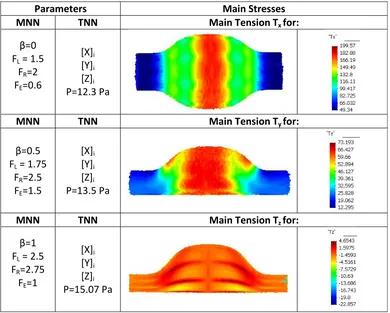
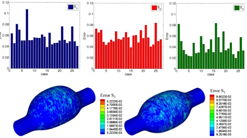
Title: Mechanical stress in abdominal aortic aneurysms using artificial neural networks. Authors: Eduardo Soudah, José F. Rodríguez, Roberto López
Journal of Mechanics in Medicine and Biology. Vol. 15, No. 3 (2015) 1550029 DOI: 10.1142/S0219519415500293
Contents
Index . . . IX
1 Introduction 3
1.1 Biomechanical forces . . . 3
1.2 Diagnostic Indicators . . . 4
1.2.1 Clinical practice & Diagnostic Indicators . . . 9
1.2.2 Coronary Artery Disease . . . 10
1.3 Objectives . . . 14
1.4 Methodology . . . 16
1.4.1 Patient-specific modelling . . . 16
1.4.2 Computational hemodynamics . . . 17
1.4.3 Postprocessing . . . 20
2 A Reduced Order Model based on Coupled 1D/3D Finite Element Simulations for an Efficient Analysis of Hemodynamics Problems. 21 3 CFD Modelling of Abdominal Aortic Aneurysm on Hemodynamic Loads using a Re-alistic Geometry with CT. 31 4 Modelling human tissues an efficient integrated methodology. 41 5 Mechanical Stress in Abdominal Aneuryms using Artificial Neural networks. 63 6 Estimation of Wall Shear Stress using 4D flow Cardiovascular MRI and Computa-tional Fluid Dynamics. 77 7 Related Work 93 7.1 Qualitative evaluation of flow patterns in the Ascending aorta with 4D phase con-trast sequences . . . 93
7.1.1 Conclusions. . . 95
7.2 Study new mechanical factor related to the Abdominal Aortic Aneurysm . . . 97
7.2.1 Conclusions. . . 99
7.3 Computational fluid dynamics in coronaries . . . 101
7.3.1 Conclusions. . . 102
IX
8 Conclusions and Future work 105
8.1 Conclusions . . . 105
8.2 Limitations and Future work . . . 106
Appendix 109 A Cardiovascular physiology 109 A Cardiovascular physiology . . . 109
A.1 Blood Vessels . . . 110
A.2 Blood Modelling . . . 112
B Numerical Model 115 B 1D Mathematical Model . . . 115
B.1 Conservation equations. . . 117
B.2 Conservation of the mass . . . 117
B.3 Conservation of the momentum . . . 118
B.4 Vessel wall constitutive model . . . 120
B.5 Characteristic analysis . . . 123
B.6 Boundary conditions . . . 126
B.7 Implementation . . . 129
B.8 Coupling 1-D and 0-D models . . . 136
B.9 Validation . . . 137
C Python Script 141 C1 Phyton Script . . . 141
D Projects 145 D1 Projects . . . 145
E Publications 147 E1 Publications . . . 147
List of Figures
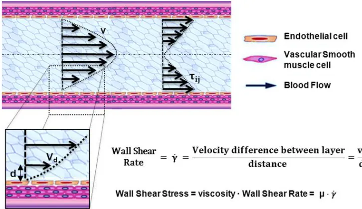
1.1 Biomechanical forces acting on the arterial wall. Blood pressure and blood flow induce forces in the vascular system that lead the initiation or progression of some cardiovascular diseases. Blood pressure produces a force directed perpendicular to the vessel wall. As a consequence, the cylindrical structure will be stretched circumferentially, resulting in a circumferential stress. In contrast, the force in-duced by a difference in movement of blood and the non-moving vessel wall leads to stress and strain parallel to the surface of endothelial cells. Due to its shearing deformation, this is called a shear stress. This shear stress exerts its main effects through the activation of mechanosensitive receptors and signalling pathways. . . 4 1.2 Hemodynamic forces that act on blood vessels. Wall shear stress (WSS) is
pro-portional to the product of the blood viscosity (µ) and the spatial gradient of blood velocity at the wall (dv/dy). . . 5 1.3 Diagnostic Indicators in a patient-specific model. . . 7 1.4 Left: Streamlines in a healthy aorta. Right: Streamlines in unhealthy aorta . . . . 8 1.5 Left, Atherosclerosis lesion. Right, Flow around rectangular section of stent . . . 10 1.6 Streamline and wall shear stress in a coronary artery. . . 11 1.7 Diagnostic Indicators in Aortic Abdominal Aneurysm. Streamlines, wall shear
stress and velocity profiles at different section of the aneurismatic sac.[87] . . . . 12 1.8 Left CT DICOM (sagital, coronal and axial images) of patient with Aortic
Ab-dominal Aneurysm. Center CT volume render of Aortic AbAb-dominal Aneurysm illustrating the Abdominal sac. Right computational patient-specific model and computational mesh . . . 16 1.9 From the medical image to the simulation . . . 19 1.10 Coupling of 0D heart model, with 1D model (Systemic Circulation), 3D model
(patient-specific geometry) and 0D lumped models (terminal resistance) to per-form a computational analysis . . . 20
7.1 Blood flow patterns in ascending aorta, left (velocity vector), right (streamlines). A and B show a laminar flow with maximum speed in the center of the aortic flow. C and D show a turbulent flow into the dilation of the aorta with an eccentric jet. D and E show a turbulent flow into the elongation of the aorta with an eccentric jet. 94 7.2 Left, Aortic index versus flow characteristics. Right, Aortic elongation versus flow
characteristics. . . 95
LIST OF FIGURES XI
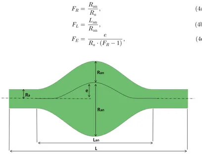
7.3 Abdominal Aneuryms 1D geometrical parameters. D: maximum transverse diam-eter, Dpn: neck proximal diameter(smallest diameter of the infrarenal artery, just before the AAA), Ddn: neck distal diameter (smallest diameter of the aorta, just after the AAA), L: aneurismal length (length between proximal and distal necks), Dli: left iliac diameter (left iliac diameter), Dri: right iliac diameter (right iliac
diameter) andαis the angle between the right and left iliac arteries. . . 97
7.4 Spatial distribution of WSS, OSI, ECAP and RRT in three abdominal aortic aneurysm. For each AAA, anterior and posterior views of the lesions. On the right, 3D vol-ume render and a CT slice showing the localization of the incipient thrombus (red line: thrombus, blue line: lumen). Dark Blue line represents the localization of the CT slice. . . 99
7.5 Methodology proposed to compute pressure drop in the coronaries . . . 102
7.6 Spatial distribution of OSI, RRT and ECAP in an right coronary artery. . . 102
8.1 Preliminary concept of automatic segmentation of the Aorta based on 4D MRI data 108 A1 The cardiovascular system is a close loop. The heart is a pump that circulates blood through the system. Arteries take blood away from the heart (systemic circulation) and veins (pulmonary circulation) carry blood back to the heart[39].. 110
A2 The human circulatory system (simplified). Red indicates oxygenated blood (ar-terial system), blue indicates deoxygenated (venous system)[106]. . . 112
B1 Section of an artery with the principal geometrical parameters . . . 116
B2 Blood flow profile adopting different values ofγ. . . 119
B3 Diagram of characteristics in the (z,t) plane. The solution on the point Ris ob-tained by the superimposition of the two characteristicsW1andW2. . . 125
B4 Boundary and initial conditions of the hyperbolic system. . . 126
B5 One-dimensional model with absorbing conditions. . . 126
B6 1-D arterial vessel domain (left) and the equivalent 0-D system discretises at first order in space (right). . . 128
B7 One-dimensional mesh representing a vessel. . . 130
B8 Sketch of a 1D linear shape function. . . 131
B9 Domain decomposition of a bifurcation 1-2. . . 133
B10 Domain decomposition of a bifurcation 1-1. . . 135
B11 Coupling 1-D/0-D model. . . 136
B12 a) Plan view schematic of the hydraulic model. 1: Pump (left heart); 2: catheter access; 3: aortic valve; 4: peripheral resistance tube; 5: stiff plastic tubing (veins); 6: venous overflow; 7: venous return conduit; 8: buffering reservoir; 9: pulmonary veins. (b) Topology and references labels of the arteries simulated, whose proper-ties are given in table B2. (c) Detail of the pump and the aorta [61]. . . 138
List of Tables
7.1 Geometrical parameters of the 13 AAA cases analyzed . . . 98
A1 Vessel Type . . . 111
B1 Analogy between hydraulic and electrical network [46]. . . 129 B2 Properties of the 37 silicon vessels used in the in-vitro model [61]. The interval of
confidence of the geometrical measurements is indicated in the heading. . . 140
Abstract
In recent years, the study of computational hemodynamics within anatomically complex vascular regions has generated great interest among clinicians. The progress in computational fluid dynam-ics, image processing and high-performance computing have allowed us to identify the candidate vascular regions for the appearance of cardiovascular diseases and to predict how this disease may evolve. Medicine currently uses a paradigm called diagnosis. In this thesis we attempt to intro-duce into medicine the predictive paradigm that has been used in engineering for many years. The objective of this thesis is therefore to develop predictive models based on diagnostic indicators for cardiovascular pathologies.
We try to predict the evolution of aortic abdominal aneurysm, aortic coarctation and coronary artery disease in a personalized way for each patient. To understand how the cardiovascular pathol-ogy will evolve and when it will become a health risk, it is necessary to develop new technologies by merging medical imaging and computational science. We propose diagnostic indicators that can improve the diagnosis and predict the evolution of the disease more efficiently than the meth-ods used until now. In particular, a new methodology for computing diagnostic indicators based on computational hemodynamics and medical imaging is proposed. We have worked with data of anonymous patients to create real predictive technology that will allow us to continue advancing in personalized medicine and generate more sustainable health systems. However, our final aim is to achieve an impact at a clinical level. Several groups have tried to create predictive models for cardiovascular pathologies, but they have not yet begun to use them in clinical practice. Our objective is to go further and obtain predictive variables to be used practically in the clinical field.
It is to be hoped that in the future extremely precise databases of all of our anatomy and phys-iology will be available to doctors. These data can be used for predictive models to improve diagnosis or to improve therapies or personalized treatments.
Resumen
Durante los últimos años, el estudio de las enfermedades cardiovasculares mediante el uso técnicas computacionales ha generado muchas expectativas en el campo de la medicina. Los avances real-izados en técnicas de procesamiento de imágenes, métodos computacionales y el uso de grandes procesadores de cálculo han permitido identificar y correlacionar variables hemodinámicas con los estados incipientes o de desarrollo de patologías cardiovasculares. Hoy en día la medicina se basa en el diagnóstico, pero en esta tesis queremos tratar de introducir el concepto de medicina computacional preventiva. El objetivo principal es desarrollar modelos preventivos basados en indicadores de diagnóstico para patologías car-diovasculares combinando procesamiento de imá-genes y técnicas computacionales.
En esta tesis, tratamos de predecir la evolución de aneurismas abdominales o la formación del trombo intraluminal en el interior del saco aneurismático, estudio de la ateroesclerosis y de la coartación de aorta, así como, posibles problemas derivados de la válvula aórtica de manera personalizada a cada paciente. Para entender cómo una patología cardiovascular evolucionará y cuándo va a convertirse en un riesgo para la salud, es necesario desarrollar una metodología efi-ciente que permita calcular indicadores de diagnóstico. En esta tesis, hemos propuesto indicadores de diagnóstico basados en técnicas computacionales e imágenes médicas que pueden mejorar el diagnóstico y a la vez podrían predecir la evolución de una patología de manera más eficiente que los métodos utilizados hasta ahora. Sin embargo, el objetivo final es llevar dichos indicadores a la práctica clínica. Actualmente estamos trabajando con datos de pacientes anónimos para crear una gran base de datos que nos permita avanzar en la medicina personalizada y en la generación de sistemas de salud más sostenibles. Es de esperar que en el futuro existan estas bases de datos a disposición de los médicos, y que estos datos se puedan utilizar para mejorar el diagnóstico o para mejorar terapias o tratamientos personalizados.
Resum
En els últims anys, l’estudi de l’hemodinàmica computacional en regions vasculars anatòmicament complexes ha generat un gran interès entre els clínics. El progrés obtingut en la dinàmica de fluids computacional, en el processament d’imatges i en la computació d’alt rendiment ha permès identi-ficar regions vasculars on poden aparèixer malalties cardiovasculars, així com predir-ne l’evolució. Actualment, la medicina utilitza un paradigma anomenat diagnòstic. En aquesta tesi s’intenta in-troduir en la medicina el paradigma predictiu utilitzat des de fa molts anys en l’enginyeria. Per tant, aquesta tesi té com a objectiu desenvolupar models predictius basats en indicadors de diag-nòstic de patologies cardiovasculars.
Tractem de predir l’evolució de l’aneurisma d’aorta abdominal, la coartació aòrtica i la malal-tia coronària de forma personalitzada per a cada pacient. Per entendre com la patologia cardio-vascular evolucionarà i quan suposarà un risc per a la salut, cal desenvolupar noves tecnologies mitjançant la combinació de les imatges mèdiques i la ciència computacional. Proposem uns in-dicadors que poden millorar el diagnòstic i predir l’evolució de la malaltia de manera més eficient que els mètodes utilitzats fins ara. En particular, es proposa una nova metodologia per al càlcul dels indicadors de diagnòstic basada en l’hemodinàmica computacional i les imatges mèdiques. Hem treballat amb dades de pacients anònims per crear una tecnologia predictiva real que ens per-metrà seguir avançant en la medicina personalitzada i generar sistemes de salut més sostenibles. Però el nostre objectiu final és aconseguir un impacte en lŠàmbit clínic. Diversos grups han tractat de crear models predictius per a les patologies cardiovasculars, però encara no han començat a utilitzar-les en la pràctica clínica. El nostre objectiu és anar més enllà i obtenir variables predic-tives que es puguin utilitzar de forma pràctica en el camp clínic.
Es pot preveure que en el futur tots els metges disposaran de bases de dades molt precises de tota la nostra anatomia i fisiologia. Aquestes dades es poden utilitzar en els models predictius per millorar el diagnòstic o per millorar teràpies o tractaments personalitzats.
Chapter 1
Introduction
Clinical evidences have always allowed us to identify the candidate vascular regions for the ap-pearance of cardiovascular diseases and to predict how these diseases may evolve. These clinical evidences are usually based on biological markers or anatomical indicators. However, over the last few years, thanks to the progress in computational hemodynamics, imaging processing, ge-ometry reconstruction techniques and the increase in high-performance computing, variables such as, wall shear stress, wall elasticity, vorticity, turbulent kinetic energy, flow patterns or pressure drop, among others, have become new clinical evidences or diagnostic indicators (DIs), espe-cially for cardiovascular diseases (CVD). Previously, patient-specific simulations were typically applied in advanced stages of disease progression, and consequently, from a medical point of view were a diagnosis-costly ineffective. In that sense, computational hemodynamics has emerged as a promising tool to estimate these new DIs and it’s playing a key role in the understanding of CVD hemodynamics. The correlation of these new DIs with patient-specific data is needed to predict the development of cardiovascular pathologies and to improve the surgical strategies. In fact, these DIs are increasingly becoming a clinical reference standard for early diagnosis, treat-ment and prognosis allowing a better stratification of patients with disease stage adapted therapy instead of escalating to the most aggressive and costly therapy. Therefore, the precise knowledge and understanding of computational hemodynamics has become a necessity of the medical com-munity, which includes the cardiovascular physiology, medical imaging and Computational Fluid Dynamics (CFD).
The purpose of this chapter is to give an outline of the most common diagnostic indicators used in cardiovascular diseases, as well as, the objectives and the methodology used in this thesis.
1.1
Biomechanical forces
It is well-known that the interactions of pulsatile blood flow with arterial geometries generate complex biomechanical forces on the vessel wall with spatial and temporal variations. Those biomechanical forces act over the internal layer of the arteries, endothelium. The endothelium produces a wide array of biochemical signals (homeostatic mediators) under physiological
ditions [102][21] keeping the artery healthy. A key stimulus to maintain the protective status of the endothelial lining at the inner vessel wall is the tangential force that blood flow exerts on it; this tangential force is known as wall shear stress (WSS) (figure 1.1). Fluctuations of the wall shear stress provoke changes in the biochemical signals[104], may arise the initiation and progres-sion some cardiovascular diseases. For example, the growth or possibly rupture of the aneurysm wall[40], plaque instability in the carotid bifurcation[16][15] or in the coronaries [35][103], throm-bus formation[41][22] or playing an important role in atherogenesis[3][10]. From a clinical stand point, the assessment of hemodynamic forces within the cardiovascular system circulation is still a challenge for the medical community, due to the three dimensional blood flow patterns close to the arterial wall needs to be measured in vivo. For that reason, computational hemodynamics has emerged as important tool for the clinician, allowing to quantify those hemodynamic forces and to correlate with the progression of cardiovascular pathologies.
Figure 1.1:Biomechanical forces acting on the arterial wall. Blood pressure and blood flow induce forces in the vascular system that lead the initiation or progression of some cardiovascular diseases. Blood pressure produces a force directed perpendicular to the vessel wall. As a consequence, the cylindrical structure will be stretched circumferentially, resulting in a circumferential stress. In contrast, the force induced by a difference in movement of blood and the non-moving vessel wall leads to stress and strain parallel to the surface of endothelial cells. Due to its shearing deformation, this is called a shear stress. This shear stress exerts its main effects through the activation of mechanosensitive receptors and signalling pathways.
1.2
Diagnostic Indicators
1.2. DIAGNOSTIC INDICATORS 5
τij = 2·µ·dij =µ
δui
δxj + δuj
δxi
(1.1)
whereµis fluid dynamic viscosity, whereuthe fluid velocity,δ/xi,j is the distance to the vessel wall andτij is the wall shear stress. Ifτij is proportional to the deviatoric stress tensor (relation between the shear stress and the strain rate is linear), the fluid is known as Newtonian fluid. And when the relation between the deviatoric shear stress and the strain rate tensor is nonlinear, the fluid is known as Non-Newtonian fluid. Therefore, the relationship between the deviatoric stress tensor and the strain rate tensor models defined the rheological behavior of a fluid. Perktold et al.[70] pointed out how the errors deriving from employing a Newtonian model for blood yield non-essential differences in flow characteristics and wall shear stress distributions. In this thesis, a rigid wall (no slippage is allowed) and blood (see appendixA) as Newtonian fluid are considered, therefore WSS can be defined as:
τij =WSS=µ·γ˙ =µ·
δuj
δxi
(1.2)
[image:24.595.124.487.419.629.2]where γ˙(sec−1) is the shear rate (δuj/δxi), whereuj is the parallel blood fluid velocity to the wall and xi the normal distance to the arterial wall. Figure 1.2 shows the blood flood hemody-namic forces acting on vessel wall. When analyzing a cardiac flow (pulsating flow), it may be of
Figure 1.2:Hemodynamic forces that act on blood vessels. Wall shear stress (WSS) is proportional to the product of the blood viscosity (µ) and the spatial gradient of blood velocity at the wall (dv/dy).
patient to allow comparison among different patients[87][108]
T AW SS= 1
T ·
Z T
0
WSS·dt
(1.3)
where WSS is the instantaneous shear stress vector and T is the duration of the cycle. Another parameter related to WSS oscillations is the oscillatory shear index (OSI)[16]:
OSI = 1 2
1−
RT
0 WSS·dt
RT
0 |WSS| ·dt
(1.4)
Oscillatory shear index is used to identify regions on the vessels wall subjected to highly oscil-lating WSS values during the cardiac cycle. For example, a purely oscillatory flow with equal forward and backward contributions will produce an OSI of 0.5; however, in unidirectional flows the OSI will be identically zero. High OSI induces region with perturbed endothelial alignment. These regions are usually associated with bifurcations flows and vortex formation that are strictly related to atherosclerotic plaque formation and fibrointimal hyperplasia.
Based on wall shear stress, and its temporal and spatial variations, other indices have been pro-posed to capture the mechanobiological effects over the endothelium[53], such us, relative res-idence time(RRT)[37], particle residence time(PRT)[91] or endothelial cell activation potential (ECAP)[22]. Relative Residence Time (RRT) is defined as the state of disturbed flow. The resi-dence time of the blood near the wall is reflected by combination of WSS and OSI. Mathematically, RRT is inversely proportional to the magnitude of the time-averaged WSS vector:
RRT = 1
(1−2·OSI)·T AW SS (1.5)
The particle residence time describes flow stagnation or recirculation, for example in the abdomi-nal aneurysm [22] or cerebral aneurysm [90]. ECAP is defined the endothelial susceptibility, and correlate the TAWSS with the OSI:
ECAP = OSI
T AW SS (1.6)
The main purpose of this index is to identify local regions of the wall that can be exposed to pro-thrombotic WSS stimuli. Higher values of the ECAP index will thereby correspond to situations of large OSI and small TAWSS, that is, i.e. in abdominal aneurysm, intraluminal thrombus (ILT) development.
1.2. DIAGNOSTIC INDICATORS 7
of WSS is still challenging in complex flow geometries [74][58][7][65]. For that reason, a good modelization combined with a numerical simulation is still needed.
Figure 1.3:Diagnostic Indicators in a patient-specific model
Other importance feature in many cardiovascular diseases is the helical flow patterns and turbulent blood flow, characterized by fast random temporal and spatial velocities fluctuations[64]. These irregular and rapid fluctuations are not present in healthy situations, and play also a key role in some cardiovascular pathologies. The helical flow patterns show a measure(index) of blood flow complexity, and therefore, is an important factor in the development of cardiovascular disease, as shown in figure1.4. Given the fluid flow velocity vector fieldu, the vorticity vector fieldwis the curl of the velocity field:
w=∇ ×u (1.7)
Basically, the vorticity vector points along the axis of spin, and the magnitude of the vorticity vector encodes the rate of spin. Given the vorticity vector field, mathematicians introduce several useful additional concepts: vortex lines, vortex sheets and vortex tubes. Technically speaking, vortex lines are the integral curves of the vorticity vector field; this simply means that vortex lines are curves which are tangent to the vorticity field at each point. Vortex sheets, meanwhile, are surfaces which are tangent to the vorticity field at all points. Vortex tubes are three-dimensional regions obtained by taking a 2 dimensional area orthogonal to the vorticity field, and then taking all the vortex lines through that area. Now, thehelicity (h)is defined as the inner product of the velocity and the vorticity:
h=u w (1.8)
vortex tube can be defined by integrating the helicity field:
H=
Z
u·(∇xu)·d3r (1.9)
It is a theorem of inviscid fluid mechanics that the helicity of a vortex tube is preserved over time. However, if a vortex tube is stretched, then its cross sectional area decreases, and the magnitude of the vorticity w increases, lowering the pressure at the center of the vortex. So, from a blood flow dynamics, the stretching of longitudinal vortex tubes could be a indicators of a cardiovascular pathology [4]. These effects are directly correlated with the oscillatory shear index [16].
Figure 1.4:Left: Streamlines in a healthy aorta. Right: Streamlines in unhealthy aorta
Another index to evaluate blood complexity is to measure the Turbulent Kinetic Energy (TKE). The velocity and the turbulent kinetic energy combined can give a visualization of disturbed flow. Increased level of TKE indicates more turbulent flow, and it is undesirable for the cardiovascu-lar system. For this reason, analyzing and understanding energy transfer and dissipation in some cardiovascular pathologies is important for the clinician. From mathematical point of view, the turbulent kinetic energy is calculated and defined as half sum of the variance of the velocity fluc-tuations:
T KE = 1
2·(u02+v02+w02) (1.10)
1.2. DIAGNOSTIC INDICATORS 9
For that reason, computational hemodynamic becomes a promising tool to estimate the pressure non-invasively. For example, pressure-derived myocardial Fractional Flow Reserve index(FFR) is the standard goal for determining the physiological significance of a coronary stenosis[73]. FFR index is calculated as the ratio of the distal pressure to the stenosis/coartaction by the proximal pressure to the lesion in a non-rest situation (or maximum effort). Furthermore, the clinicians are able to reproduce several patient-conditions modifying the boundary conditions of computational model, based only on a medical image. The clinicians should simulate a non-inducing stress sit-uation to the patient reducing the intervention costs. The capability of computing the pressure drop without pressure-wire has gained wide acceptance in the clinical community in the recent years[94][100].
1.2.1 Clinical practice & Diagnostic Indicators
The purpose of this section is doing a review of how the Diagnostic Indicators (above mentioned) can be applied into a clinical practice.
1.2.1.1 Atherosclerosis
Figure 1.5: Left, Atherosclerosis lesion. Right, Flow around rectangular section of stent
coronary arteries linked with the coronary stenosis. In [69] there is a review comparing the lo-calization of atherosclerotic lesions with the distribution of haemodynamic indicators calculated using computational fluid dynamics.
1.2.2 Coronary Artery Disease
Coronary artery disease(CAD) is the most common type of heart disease and cause of heart at-tacks. CAD is caused by abnormal narrowing of the coronary arteries (coronary stenosis) resulting in reduction of blood flow to the heart. The stenosis impedes to deliver oxygen to the heart mus-cle, which provoking heart attack. This disease is directly related with the atherosclerosis plaque. When stenosis occurs, the common clinical practice for decision taking related to the need (or not) of implanting a stent in a obstructed coronary artery requires the measurement of the Fractional Flow Reserve (FFR). FFR is derived from measuring the ratio of aortic pressure and pressure beyond a stenosis. Stenting is a specialized treatment for coronary arteries that are narrowed or blocked by plaques. It involves placing a balloon into the narrowed portion of the coronary artery with a surrounding wire mesh (stent). When the balloon is expanded, the stent remains in the vessel keeping the plaque pushed outwards, to let blood flow to the heart pass by.
1.2. DIAGNOSTIC INDICATORS 11
Figure 1.6:Streamline and wall shear stress in a coronary artery
for such methods are the lack of patient-specific data including anatomy, patient-specific boundary conditions, the condition of the microvasculature of the myocardium, and the large-scale compu-tational resources required for the complex calculations. In [92] pressure gradients are computed using CFD in which the geometry of the aorta is extracted from MRA. Additional MR Phase con-trast imaging is performed to measure the velocity which is used as boundary conditions. In [94], lumped parameter models of the heart, systemic circulation and coronary microcirculation are coupled to a patient specific 3D model of the aortic root and epicardial coronary arteries extracted from CTA. Disadvantages of these approaches are that all calculations are performed exclusively in 3D as well as the fact that the calculations cannot be performed during intervention because of the need for CT. Moreover, one vital piece of information is still missing in CFD, namely the con-dition of the coronary circulatory auto-regulation, also known as the patients cardiac flow reserve. This results in a method that is of high computational complexity. A recent study applied CFD to three dimensional X-ray angiography for the computation of the FFR incorporating the coronary flow reserve[98] . However, this method requires X-ray angiographic imaging during hyperemia which is a burden to the patient. Placing known side effects of adenosine into perspective; reduced blood flow to the heart which might worsen symptoms in patients with coronary heart diseases or even cause a heart attack, this is clearly an undesired situation especially during diagnostic coronary angiography.
1.2.2.1 Aortic Aneurysms
aorta is termed a Thoracic Aortic Aneurysm(TAA), in the abdominal aorta is named Abdominal Aortic Aneurysm(AAA). However, the aneurysm pathogenesis is still unknown. It is thought that
Figure 1.7: Diagnostic Indicators in Aortic Abdominal Aneurysm. Streamlines, wall shear stress and velocity profiles at different section of the aneurismatic sac.[87]
1.2. DIAGNOSTIC INDICATORS 13
1.2.2.2 Aortic Coarctation
1.3
Objectives
The general objective in this thesis is improving computational hemodynamics to develop pa-tient specific diagnostic indicators for an early identification of cardiovascular incumbent physio-pathological state (and its progress). To reach this goal, this thesis attempts to improve the prior mathematical models used for cardiovascular system for a deeper understanding on the response of the cardiovascular system to:
• improve diagnostics and therapeutical procedures for Aorta Coarctation (paper 1 in Chapter 2),
• study the mechanical factors that may be important in triggering the onset of aneurysms (paper 2 in Chapter 3 and paper 4 in Chapter 5),
• combine medical images with computational hemodynamic to estimate DI’s (Chapter 6) and
• use medical images data to generate computational model (paper 3 in Chapter 4).
Other applications studied based on the methodology developed in this work were, (i) a new method to estimate the fractional flow reserve (FFR) using CFD data, (ii) study of new mechanical factor related to the AAA and (iii) studied the effect of vorticity and the eccentricity of the aortic bicuspid valve (in Chapter7).
From the methodology point of view, a new methodology to compute diagnostic indicators based on computational hemodynamics has been proposed. In order to compute the pressure drop under different patient-specific situations, a reduced-order model has been developed in paper 1. The reduced-order method was implemented as part of the C++ finite element library KRATOS[17]. KRATOS is a multiphysics simulation open source (LGPL licence) framework based on the stabi-lized Finite Element Method for analysis of the Navier-Stokes equations in viscous flows. Efficient and parallel solvers for 3D fluid problems have been implemented in KRATOS that allow tackling large problems using supercomputers if available. The 1D model developed in this thesis was also implemented as new elements inside KRATOS. Blood was modeled as a Newtonian fluid with constant density and different outlet conditions were implemented. In Appendix Ba detail de-scription of the implementation is shown.
1.3. OBJECTIVES 15
comprehensive descriptions of the flow fields than any other in-vivo imaging technique (in chapter 7). The velocity data provided by 4D flow CMR has been complementary to the higher resolution velocity fields computed by the CFD in order to estimate the WSS. We have also developed an algorithm to compute WSS based on the 4D flow CMR data. To compute vorticity and helicity from a velocity field a Vascular Modeling Toolkit (VMTK) [4] was used. In spite of this, a new diagnostic indicator to estimate coronary artery disease based on computational hemodynamics has been also proposed (in chapter7).
1.4
Methodology
1.4.1 Patient-specific modelling
Patient-specific modeling is the development of computational models of human physiology that are individualized to patient-specific data. Imaging data can be stored in the Digital Imaging and Communication in Medicine (DICOM) format [6]. The DICOM format file contains two parts: the header which stores detailed information about the patient such as name, type of scan, ages, dimension of the image and the voxel, image position, and so forth. The second data set contains information of each scanned image. Segmentation of medical image was required to extract the geometry of the region of interest (or analysis). The segmentation process can include several procedures as threshold, region growing, centerline, among others, followed by 3D anatomical reconstruction to obtain a coarse solid model. During threshold, a range of gray scale values are selected such that the region to be selected is of the best contrast. After the regions of interest are extracted, the voxels are labelling together with an identificator to create the 3D geometry.
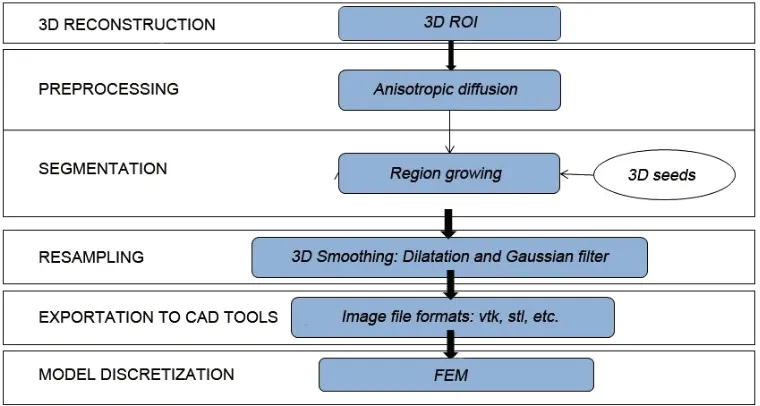
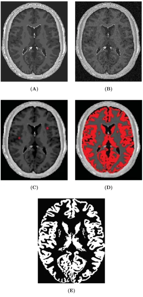
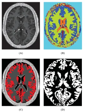
In paper 3 an efficient methodology for preprocessing and postprocessing medical images to gen-erate computational meshes for numerical simulation is explained. A schematic flowchart for creating and validating a 3D patient-specific model is shown in Figure 5 of paper 3. Aneurysm models (patient-specific geometries) of paper 2 were reconstructed from computer tomography-angiography (CTA) scans using the diagnostic software ITK-SNAP[109] and DIPPO[13].
Figure 1.8: Left CT DICOM (sagital, coronal and axial images) of patient with Aortic Abdominal Aneurysm. Center CT volume render of Aortic Abdominal Aneurysm illustrating the Abdominal sac. Right computational patient-specific model and computational mesh
1.4. METHODOLOGY 17
coronary artery disease. The 3D model reconstructed was based on two bi-dimensional images taken from different perspectives. Then the reconstruction of abdominal aneurysm anatomy or coronary into a computational mesh (computer model) is performed based on the segmentation information. To generate the computational mesh GiD Pre and Postprocessor [13] and the open source Vascular Modeling Toolkit (VMTK) [4] were used.
Next, a list of freely available tools for medical image processing and mesh generation using in the appended papers is outlined; VTK[83] is an open-source software toolkit for visualization, computer graphics and image processing with a great online community and numerous examples. VTK is cross platform with implementations for Windows, Mac Os and Linux. Users can code in C++, Java, Phyton or TCL. Knowlegde of VTK means that developers can take advantage of other tools sush as ITK, ITK-SANP or IGSTK[25], to name a few. ITK[38] is an open-source, cross-platform system that sits on top of VTK. It provides developers with an extensive suite of software tools for image analysis. ITK-SNAP[109] is a freely available tool built on ITK and VTK for image manipulation. The source code for ITK-SNAP is part of ITK Applications, so develop-ers can add their own modifications. DCMTK[1] is a collection of libraries and applications for reading, writing and otherwise manipulating DICOM images. It works with multiple operating systems. VMTK[4] is collection of applications for pre and postprocessing medical images.
1.4.1.1 4D flow cardiovascular magnetic resonance imaging
At present, 4D flow cardiovascular magnetic resonance imaging (4D CMRI) sequences are being a promising tool to visualize and quantify 4D (3D+t) blood flow. From these sequences the raw data can be obtained and conveniently processed, allowing visualization of the blood flow patterns in any segment of the cardiovascular tree[59][50][72]. Nevertheless, the visualization of these images entails an important manual work, becoming a very time-dependent task and then turning out to be not useful in the current clinical practice. Therefore, it is important to improve the technology and the methods of automatic representation of the 4D blood flows, in particular for the WSS analysis. In chapter 6, it is demonstrated that 4D flow CMRI technique is a reliable tool to provide the boundary conditions for the Computational Fluid Dynamics(CFD) in order to estimate the WSS within the entire thoracic aorta in a short computation time. Our image-based CFD methodology exploits the morphological MRI for geometry modelling and 4D flow CMRI for setting the boundary conditions for the fluid dynamics modelling. The aim is to evaluate visualization of well-defined aortic blood flow features and the associated wall shear stress by the combination of both techniques. In that sense, CIMNE has developed a home-made ad-hoc software (Aorta4D) oriented to make progress in this field of work [50][89][72]. Aorta4D will afford analysis and spatially visualization of the registered 3-directional blood flow velocities, and perform a 3D semi-automatic segmentation based on the 4D flow CMRI data.
1.4.2 Computational hemodynamics
In this thesis, we consider blood as an homogeneous, incompressible, constant-density (ρ=1050 kg/m3) and newtonian fluid with constant viscosity (µ=0.0035 Pa.s). Vascular walls are modeled as non-permeable, rigid walls (see sectionA). Under these assumptions, the conservation of mass and momentum in the compact form are described by the following system of partial differential equations (1.11):
ρ·
∂u
∂t + (u· 5u)
+∇p− ∇ ·(µ4u) = ρ·f inΩ(0, t) ∇u = 0 inΩ(0, t)
(1.11)
whereΩ is a three-dimensional domain,u denotes the blood velocity, p is the pressure field,ρ
density,µthe dynamic viscosity of the fluid andfthe volumetric acceleration. Volumetric forces(ρ· f) and thermal effects are not considered in this thesis. The spatial discretization of the Navier-Stokes equations has been done by means of the finite element method (FEM), while for the time discretization an iterative algorithm that can be considered as an implicit fractional step method has been used [14][17]. Blood flow can be characterized by the Reynolds and Womersley [107] dimensionless number. These numbers correlate the inertial and viscous forces of the previous equation 1.11. The Womersley number is a dimensionless parameter that represents the ratio between oscillatory inertial forces and viscous forces. Physically, the Womersley number can be interpret as the ratio of artery diameter to the laminar boundary layer growth over the pulse period (characteristic frequency).
α= D 2 ·
rwρ
µ (1.12)
wherewthe characteristic frequency and D is the characteristic diameter. Ifαis high, the fluid is nonviscous, and Ifαis low, the viscosity of the fluid is high. Womersley number characterizes the unsteady of the blood flow. The ratio of the inertial force to the viscous forces is the dimensionless parameter calledReynolds number
RE= U 2ρ µu
D
= LU ρ
µ (1.13)
1.4. METHODOLOGY 19
Figure 1.9:From the medical image to the simulation
1.4.2.1 Patient-specific boundary conditions
It is well known that to estimate properly the DI’s, the specific patient-specific boundary conditions are needed. Several authors [42][76][93] have noted how inlet velocity profiles and flow waveform shapes play an non-negligible role on wall shear stress or pressure distributions. Nowadays, there are several medical techniques to perform velocity measurements inside large arteries in vivo and non-invasively, as Doppler Utrasound or phase-contrast magnetic resonance. Using this acquired data into the computational hemodynamical model will provide us enough information to perform our computational simulation. It should be pointed out that the conditions measured depend on physical activity and posture of the patient [52]. In chapter 2 and chapter 7 the technique uses to acquire the velocity information for the prescription of patient-specific boundary conditions was phase-contrast magnetic resonance.
Acquisition of boundary conditions by phase-contrast magnetic resonance: At present Car-diac Magnetic Resonance Imaging (MRI) image is the only non-invasive imaging modality that can measure 3D blood velocity in a 3D representation, and that allows visualization of spatial dis-tribution of velocity in a two-dimensional plane (2D). This technique is valuable non-invasively tool for evaluation of the cardiovascular flow patterns owing to its unique possibility to simul-taneously acquire sectional imaging without restriction, anatomy (magnitude image) and blood flow velocities(phase image) with a single scan. The majority of the commercial systems offer the bi-dimensional phase-contrast sequence to quantify blood velocity and derivative cardiac flow. These sequences are reliable and precise methods to calculate stroke volume for pulmonary/sys-temic flow ratios estimation (Qp:Qs) and to calculate volume regurgitation in valvular insufficien-cies [54][88]. At present, the phase-contrast sequences are being developed to allow obtaining information of the 4D flow (see1.4.1.1).
Figure 1.10: Coupling of 0D heart model, with 1D model (Systemic Circulation), 3D model (patient-specific geometry) and 0D lumped models (terminal resistance) to perform a computational analysis
the boundary conditions is to use reduced models, as 1D model or 0D (lumped) models. 1D and 0D models are mathematical models able to reproduce the systemic and pulmonary circulation by an 1D approach of the Navier-Stokes equations (see AppendixB) or by electrical analogy, respec-tively. Next figure1.10shows a standard approach to provide realistic local boundary conditions for 3D CFD simulations at the specific arterial domain using 1D models of the entire arterial tree, terminated with 0D models at the distal ends[99]. The values of the components (usually Resis-tance, Inductance and Capacitor) of the lumped model can be estimated from physical data of the subject [68][56]. This approach is quite used because it is capable to account for the effect of local pathological conditions on the whole circulatory system, providing realistic boundary conditions for the 3D problem [29][93][57].
1.4.3 Postprocessing
Chapter 2
A Reduced Order Model based on Coupled
1D/3D Finite Element Simulations for an
Efficient Analysis of Hemodynamics Problems.
Title: A Reduced Order Model based on Coupled 1D/3D Finite Element Simulations for an Effi-cient Analysis of Hemodynamics Problems.
Authors: E.Soudah, R.Rossi, S.Idelsohn, E.Oñate.
Journal: Journal of Computational Mechanics. (2014) 54:1013-1022.
Received: 18 February 2014 / Accepted: 30 April 2014 / Published online: 23 May 2014 DOI: 10.1007/s00466-014-1040-2
Scientific contribution: Design of a new methodology to estimate the pressure drop in aortic coarctation under different scenarios. The methodology is based on the integration a 1D numeri-cal model (see appendixB) into a reduced order model based on 3D CFD formulation.
Contribution to the paper:The principal author developed and implemented the 1D model and the reduced order model into the KRATOS Multi-Physics software (www.cimne.com/kratos)([17]).
Article reprinted with permission. Electronic version of an article published as: ©copyright Springer-Verlag Berlin Heidelberg 2014. Print ISSN 0178-7675. Online ISSN 1432-0924. Journal No: 00466 http://www.springer.com/
DOI 10.1007/s00466-014-1040-2
O R I G I NA L PA P E R
A reduced-order model based on the coupled 1D-3D finite element
simulations for an efficient analysis of hemodynamics problems
Eduardo Soudah · Riccardo Rossi · Sergio Idelsohn · Eugenio Oñate
Received: 18 February 2014 / Accepted: 30 April 2014 / Published online: 23 May 2014 © Springer-Verlag Berlin Heidelberg 2014
Abstract A reduced-order model for an efficient analysis of cardiovascular hemodynamics problems using multiscale approach is presented in this work. Starting from a patient-specific computational mesh obtained by medical imaging techniques, an analysis methodology based on a two-step automatic procedure is proposed. First a coupled 1D-3D Finite Element Simulation is performed and the results are used to adjust a reduced-order model of the 3D patient-specific area of interest. Then, this reduced-order model is coupled with the 1D model. In this way, three-dimensional effects are accounted for in the 1D model in a cost effective manner, allowing fast computation under different scenar-ios. The methodology proposed is validated using a patient-specific aortic coarctation model under rest and non-rest con-ditions.
Keywords Blood flow·Boundary conditions· Reduced-order models and Aortic coarctation
1 Introduction
The simulation of blood flow problems assumes a large importance in biomechanics due to the many potential fields of application. The use of realistic boundary conditions is essential to guarantee the performance and the accuracy of numerical simulations, especially in cardiovascular
prob-E. Soudah·R. Rossi·S. Idelsohn·E. Oñate
International Center for Numerical Methods in Engineering (CIMNE), Technical University of Catalonia, 08034 Barcelona, Spain
e-mail: esoudah@cimne.upc.edu
S. Idelsohn (
B
)Institució Catalana de Recerca i Estudis Avançats (ICREA), Barcelona, Spain
e-mail: sergio@cimne.upc.edu
lems. In particular, the flow in arteries depends strongly on the outflow boundary conditions which model the down-stream domain. The application of constant tractions as outlet boundary conditions for 3D domains represents the simplest possibility. Unfortunately, such conditions are not realistic and cause spurious pressure waves to become in the solution. Such waves travel along the artery network and distort the numerical solution. An efficient technique is thus needed to minimize these effects. Sophisticated outlet boundary
con-ditions [29,30] aimed to minimizing such problem can be
found in the literature. Others authors address the problem by applying geometrical multiscale modeling [4,7,9,17,34,36]. These approaches typically consist in the combination of models with different levels of approximation (3D, 1D and 0D models) each aimed at capturing particular features of the solution. 3D models are applied in regions where details of the local flow are needed. This is typically the case when the flow is strongly three dimensional or it tends to be tur-bulent. 1D models are typically used in the up-downstream domain of the 3D models, so that the whole arterial network can be described efficiently taking into account flow propa-gation effects. Zero dimensional models (or lumped models) are generally used to describe the lower level of the cardio-vascular system or to model the heart. A typical problem that rises at the interface between the 1D and 3D domains is the mapping of the parabolic velocity distribution (assumed in the 1D model) to an “equivalent” distribution on the 3D inlet. Such mapping is not trivial since the discretized 3D model is generally not exactly circular. A proposal to solve
the impasse can be found in [2]. In current work we opted
topol-1014 Comput Mech (2014) 54:1013–1022
ogy of the artery or area of interest. We also observe that the method we propose works under the assumption that the 3D inlet and outlet boundaries are approximately perpendicular to the centerline of the artery and positioned at points in which the flow can be reasonably approximated as 1D. It is inter-esting to remark that, as observed in the extensive review paper [18,31], the reliable computation of WSS, which is often the target of CFD simulations, depends on the availabil-ity of a sufficiently fine discretization of the boundary layer and is sensibly affected by the Fluid-Structure Interaction of the flow with the artery boundaries. The idea we leverage in the current work is that the extra dissipation induced by severe variations of the geometry is dominated by the appear-ance of turbulent effects within the volume. The evaluation of such effect requires a sufficiently fine discretization of the volume but does not put the extra requirements on the boundary layer mesh, and shall not be severely affected by the deformability of the walls, hence allowing the assump-tions of considering the walls rigid which greatly simplifies the simulation and reduces the runtime. In [25] an extensive review of the most popular 1D models can be found. Recently, new models have been proposed [1,20,22,28] improving the viscoelastic behavior of the walls. However, the 1D models alone are not capable to capture in an effective way the energy losses due to the 3D geometrical shapes of the arteries, e.g, in stenotic arteries, aneurysms or other cardiovascular patholo-gies, such as aorta coarctation. Nevertheless, to discretize the whole 3D cardiovascular domain or coupled fluid-structure interaction (FSI) modeling is computational expensive and unfeasible in practical applications due to the numerical chal-lenges involved. Despite its modeling shortcomings, geo-metrical multiscale models combined with patient-specific geometries remains the predominant approach for vascular blood flow. Such models allow quantifying the hemodynam-ics variables such as, flow reversal, flow separation and wall shear stress areas over the arterial wall in a non-invasive way useful for clinicians. Notable exceptions include the work of [29,32,33] on cerebral aneurysms.
In this paper, we propose a reduced-order Computational Fluid Dynamics (CFD) model specifically aimed to the esti-mation of the pressure gradient and the energy losses induced by stenosis in cardiovascular scenarios. The key features of our approach are: (1) a patient-specific anatomy and a computational mesh obtained during a routine clinical imag-ing session; (2) a coupled multiscale 0D-1D-3D model to approximate the energy losses induced by a narrowing of the artery lumen. The solution of the 3D model is used to train a reduced-order model which is aimed to capturing the pressure drop within two sections located upstream and downstream of the stenosis. Then the reduced-order model is integrated within the 1D model to create a 1D reduced-order model. Such model is able to simulate the energy losses and the flow distribution taking into account the patient-specific anatomy
in real time under different scenarios. The ultimate goal is to validate the CFD framework with the energy losses through an aortic coarctation (CoA) under resting and non-resting conditions of the patient. CoA of the aorta occurs approxi-mately in 10 % of patients with congenital heart defects and represents a narrowing of the descending aorta. Due to the reduction in the aorta descending diameter, high pressure gra-dients can appear across the CoA, resulting in an increased cardiac workload in the left ventricle during systole [14]. Investigation into the hemodynamics and bio-mechanical basis of the morbidity in CoA shows that the pressure gradi-ent is dependgradi-ent on the aorta area reduction, the flow rate and the physiological state of the patient: during non-rest condi-tions the pressure gradient can increase considerably and can provoke heart failure [13]. To measure the pressure gradient under these non-rest conditions, that are difficult to replicate in a clinic environment, is a biomedical challenge [3]. For is reason, a procedure that combines patient-specific image data and numerical tools to further understand the hemody-namics alterations, under resting and non-resting situations will allow clinicians to improve the diagnosis and define which should be the CoA treatment for the patient [14,23]. Some authors have used CFD models to study the hemo-dynamics in the CoA [12,13]. However, different numeri-cal approaches might lead to different pressure predictions. The reduced-order methodology described in this paper has been implemented as part of the C++ finite element library
KRATOS (www.cimne.com/kratos) [5]. KRATOS is a
multi-physics simulation open source (LGPL licence) framework based on the stabilized Finite Element Method for analysis of the Navier-Stokes equations in viscous flows. Efficient and parallel solvers for 3-D fluid-structure interaction (FSI)
[6] problems have been implemented in KRATOS that allow
tackling large problems using supercomputers if available.
2 Computational framework
Fig. 1 3D-1D coupled
approach schematics.Γiare the interface surfaces
The trained model is thus able to estimate the energy losses between the two areas selected in the 3D model. Once the reduced-order model is defined, a coupled 1D FSI-reduced-order model will be capable of estimating the patient-specific pressure drop under different rest or non-rest situations. The second step (computing phase) consists in setting different boundary conditions for the coupled 1D FSI-reduced-order model to estimate the pressure drop (at any point) taking in account the 3D anatomical model. This will enable us to simulate different pathological situations taking into account the energy losses produced by the 3D model. Besides, this reduced-order approach brings down the computational costs significantly. The flow diagram of this scheme is shown in Fig.1.
2.1 Mathematical model for the 1D reduced-order model
In this section we describe a non-linear 1D formulation and the reduced-order model proposed to account for the 3D effects caused by the patient-specific area of interest. In absence of branching, an artery may be considered as
a cylindrical compliant tube which extends from z=0 to
z=L, where L is the the artery length. The artery takes into account the assumptions of axial symmetry, radial displace-ments, constant pressure on each section, no body forces and dominance of axial velocity. The governing system of equations for an incompressible newtonian fluid are derived by applying conservation of mass and momentum in a 1-D impermeable and deformable tubular control volume. These equations are:
∂ A ∂t +
∂Q ∂z
=0 (1a)
∂Q ∂t + ∂ ∂z αQ2
A
+A
ρ ∂P
∂z +KR
Q A
=0 (1b)
Pext+ E ho √
1−μ2 √
A−√Ao
Ao =P (1c)
where A(z,t) is the cross-sectional area of the vessel, Q(z,t) is the mean blood flow, P is the average internal pressure
over the cross-section,α is the momentum-flux correction
coefficient, z is the axial coordinate along the vessel, t is the time,ρis the density of the blood taken as 1,050 Kg/m3 and KR is the friction force per unit length, which is
mod-eled as KR = 2π ·ν(γ +2)[8], withν being the
viscos-ity of the blood taken here as 4.5 m·Pa·s. The vessel wall is modeled as a thin, homogeneous and elastic material. Para-meters A0and h0in Eq.1(c) are the sectional area and the
wall thickness, respectively, at the reference state (P0,U0),
with P0and U0assumed to be zero, E is the Young
modu-lus andμis the Poisson’s ratio, typically taken asμ ≈0.5, which implies that the biological tissue is practically incom-pressible. In absence of detailed of patient-specific data, the wall elasticity and the thickness of the 55 largest arteries are
based on data published by Wang and Parker [35]. At each
1016 Comput Mech (2014) 54:1013–1022
Qi = d
(Qj)d (2)
Pi+1
2ρ
Qi2
Ai2 =(Pj)d+
1 2ρ
(Qj2)d
(Aj2)d
+(f3Dj(k1,k2))d
(3)
where indexes i and j denote the parent and the daugh-ter vessels respectively, and d indicates the number of sys-tem domains. Function f3D(k1,k2) denotes the energy losses
of the 3D model, where k1 and k2 are obtained by fitting
the pressure drop between the two planes defined in the
3D model. k1 and k2 are the viscous and turbulent
coeffi-cients that should be adjusted according to the pressure drop between the two planes defined in the 3D model. In this work we do not consider the inertial term. The system obtained is solved by a Newton iteration scheme, taking as the starting point the reference section area and flow, i.e:
f3Dj(k1,k2)=k1Qj+k2|Qj | Qj (4)
With simple manipulations of the differential Eq. (1) it is possible to obtain the conservative form for the tempo-ral evolution of the flow and the vessels area and discretize the system obtained using a second order Taylor-Galerkin scheme. This scheme is appropriate for this problem as it can propagate waves of different frequencies without suffer-ing from excessive dispersion and diffusion errors. A
deriva-tion of the 1D-FSI models can be found in [8] and [27].
The Taylor-Galerkin scheme requires a time step limitation in order to keep the solution stable. In this work the stabi-lization technique adopted has been the Courant Friedrichs Lewy condition (CFL condition) [21].
Δt ≤C F L min 0≤i≤N
hi max(λ1,i, λ1,i+1)
(5)
where N is the number of the elements, hi is the local
ele-ment size andλ1,i indicates the value of the eigenvalue
eval-uated at the mesh it h node of the matrix of the
conserva-tive form obtained from the derivation of the 1D-FSI model [8]. The CFL value adopted is 0.57 [21]. The 3D computa-tional analysis is performed assuming that the arterial wall is rigid. Blood is considered as an homogeneous laminar New-tonian fluid modelled by the incompressible Navier-Stokes equations using the same density and dynamic viscosity as for the 1D model. Although these are important limitations, they make the simulation effort simpler. Furthermore, the knowledge of the patient-specific mechanical properties is quite difficult, consequently the objective of this work is to determine the pressure gradient in the anatomical domain using a reduced-order model based on multiscale
model-ing. Recent studies [15] use turbulence models to predict
the kinetic energy due to the narrowing of the coarctation.
2.2 3D-1D Coupling interfaces
In order to keep the continuity in the area sections between the 3D and the 1D geometrical models, the diameters of the 1D geometrical model were firstly scaled taking into account a proportional diameter factor between the 3D and 1D geomet-rical models. The properties of the 1D geometgeomet-rical models were taken from [35]. For the training phase, at each coupling 1D-3D interface we enforce the continuity of the flow and the total pressure (Eqs.2,3). This means that at every time step tnwe compute the velocity and the pressure using the 1D
approach over the whole domainΩ1D. Then, the variables
over the interface sections (Γ1,Γ2) of theΩ1D-Ω3Ddomain
are determined (Fig.1). Following that, the 3D problem is solved inΩ3Dusing the boundary conditions obtained in the Γ1,Γ2sections from the 1D model. For the next time step
(tn+1) the process is repeated until the final simulation time
is reached. This coupling procedure is justified by the fact that the 1D domain can be considered as a passive element which absorbs the flow generated by the 3-D domain. During the training phase, pressure values atΓ1andΓ2interfaces are
stored for each time step with the objective of estimating the coefficients k1and k2of Eq.4by the least squares method.
We choose the value of f3D(k1,k2) that minimizes the sum
of the squared pressure drop from the 1D flow values com-pared to the 3D values. In Sect.3.1.3we show a pressure drop of the 3D computational values versus the predictions of the reduced-order model (Fig.3). For the computation phase, the coupled 1D coupled FSI—reduced-order model is solved by using the coefficients k1and k2estimated previously.
3 Study case: aorta coarctation
3.1 Training phase
3.1.1 Model anatomy, geometry and mesh
The physiological and geometrical data used in this work was obtained from [3].The patient was a 71 kg, 177 cm tall, 17-year old male with a mild thoracic aortic coarctation. Image data come from a 1.5-T Phillips scanner using a gadolinium-enhanced MR angiography (MRA) with the patient in the supine position. The 3D model (Fig.2) includes the ascend-ing aorta, aortic arch, descendascend-ing aorta, left subclavii, bra-chiocephalic and finally left common carotid arteries in Stereo Lithography (STL) file format. To generate the 3D
volume we used the pre and post-processor GiD [10]. GiD