Essays on Growth through creative destruction
177
0
0
Texto completo
(2) iii. Contents 1 Introduction. 1. Bibliography. 9. 2 Financial Intermediation in a Model of Growth through Creative Destruction 2.1 Introduction . . . . . . . . . . . . . . . . . . . . . . . . . . . . . . . . . . . . 2.2 The model . . . . . . . . . . . . . . . . . . . . . . . . . . . . . . . . . . . . . 2.2.1 Consumers . . . . . . . . . . . . . . . . . . . . . . . . . . . . . . . . 2.2.2 Final good sector . . . . . . . . . . . . . . . . . . . . . . . . . . . . . 2.2.3 Intermediate goods . . . . . . . . . . . . . . . . . . . . . . . . . . . . 2.2.4 Research sector . . . . . . . . . . . . . . . . . . . . . . . . . . . . . . 2.2.5 Capital market . . . . . . . . . . . . . . . . . . . . . . . . . . . . . . 2.2.6 Financing of research . . . . . . . . . . . . . . . . . . . . . . . . . . . 2.2.7 Equilibrium . . . . . . . . . . . . . . . . . . . . . . . . . . . . . . . . 2.3 Steady State Analysis . . . . . . . . . . . . . . . . . . . . . . . . . . . . . . 2.4 Dynamics . . . . . . . . . . . . . . . . . . . . . . . . . . . . . . . . . . . . . 2.5 Welfare analysis . . . . . . . . . . . . . . . . . . . . . . . . . . . . . . . . . . 2.5.1 Tax on capital . . . . . . . . . . . . . . . . . . . . . . . . . . . . . . 2.5.2 Tax on …nancial services . . . . . . . . . . . . . . . . . . . . . . . . . 2.5.3 Tax on research activity . . . . . . . . . . . . . . . . . . . . . . . . . 2.6 Conclusions . . . . . . . . . . . . . . . . . . . . . . . . . . . . . . . . . . . .. 11 11 16 17 17 17 19 21 21 25 28 34 35 38 40 42 44. Bibliography 2.7 Proofs of propositions . . . . . . . . . . . . . . . . . . . . . . . . . . . . . .. 47 52. 3 Research Policy and Endogenous Growth 3.1 Introduction . . . . . . . . . . . . . . . . . 3.2 The model . . . . . . . . . . . . . . . . . . 3.2.1 Consumers . . . . . . . . . . . . . 3.2.2 Final good sector . . . . . . . . . . 3.2.3 Intermediate goods . . . . . . . . .. 61 61 69 69 70 70. . . . . .. . . . . .. . . . . .. . . . . .. . . . . .. . . . . .. . . . . .. . . . . .. . . . . .. . . . . .. . . . . .. . . . . .. . . . . .. . . . . .. . . . . .. . . . . .. . . . . .. . . . . .. . . . . ..
(3) iv 3.2.4 Research sector . 3.2.5 Capital market . 3.2.6 Research policy . 3.2.7 Equilibrium . . . 3.3 Steady state . . . . . . . 3.3.1 Public provision 3.3.2 Public funding . 3.4 Welfare analysis . . . . . 3.5 Conclusions . . . . . . .. . . . . . . . . .. . . . . . . . . .. . . . . . . . . .. . . . . . . . . .. . . . . . . . . .. . . . . . . . . .. . . . . . . . . .. . . . . . . . . .. . . . . . . . . .. . . . . . . . . .. . . . . . . . . .. . . . . . . . . .. . . . . . . . . .. . . . . . . . . .. . . . . . . . . .. . . . . . . . . .. . . . . . . . . .. . . . . . . . . .. . . . . . . . . .. . . . . . . . . .. . . . . . . . . .. . . . . . . . . .. . . . . . . . . .. . . . . . . . . .. . . . . . . . . .. . . . . . . . . .. . . . . . . . . .. . . . . . . . . .. . . . . . . . . .. Bibliography 3.6 Distribution of relative productivities across sectors . . . . . 3.7 Proofs of propositions . . . . . . . . . . . . . . . . . . . . . 3.7.1 Propositions under the public provision assumption 3.7.2 Propositions under the public funding assumption . 3.8 Calibration . . . . . . . . . . . . . . . . . . . . . . . . . . . 3.8.1 Public provision of research . . . . . . . . . . . . . . 3.8.2 Public funding of research . . . . . . . . . . . . . . . 3.9 Results when private …rms do not invest in basic research . 3.9.1 Public provision of research . . . . . . . . . . . . . . 3.9.2 Public funding of research . . . . . . . . . . . . . . .. . . . . . . . . . .. . . . . . . . . . .. . . . . . . . . . .. . . . . . . . . . .. . . . . . . . . . .. . . . . . . . . . .. . . . . . . . . . .. . . . . . . . . . .. 98 . 101 . 103 . 103 . 111 . 114 . 115 . 120 . 122 . 123 . 127. 4 Technological Progress and the Distribution of Productivities across tors 4.1 Introduction . . . . . . . . . . . . . . . . . . . . . . . . . . . . . . . . . . 4.2 The model . . . . . . . . . . . . . . . . . . . . . . . . . . . . . . . . . . . 4.2.1 Consumers . . . . . . . . . . . . . . . . . . . . . . . . . . . . . . 4.2.2 Final good sector . . . . . . . . . . . . . . . . . . . . . . . . . . . 4.2.3 Intermediate goods . . . . . . . . . . . . . . . . . . . . . . . . . . 4.2.4 Research sector . . . . . . . . . . . . . . . . . . . . . . . . . . . . 4.2.5 Capital market . . . . . . . . . . . . . . . . . . . . . . . . . . . . 4.2.6 Public sector . . . . . . . . . . . . . . . . . . . . . . . . . . . . . 4.2.7 Distribution of relative productivity coe¢cients . . . . . . . . . . 4.3 Equilibrium . . . . . . . . . . . . . . . . . . . . . . . . . . . . . . . . . . 4.3.1 Equilibrium under the average assumption. . . . . . . . . . . . . 4.3.2 Equilibrium under the aggregate assumption. . . . . . . . . . . . 4.4 Steady state analysis . . . . . . . . . . . . . . . . . . . . . . . . . . . . . 4.4.1 Steady state analysis under the average assumption . . . . . . . 4.4.2 Steady state analysis under the aggregate assumption . . . . . . 4.5 Conclusions . . . . . . . . . . . . . . . . . . . . . . . . . . . . . . . . . .. 72 75 76 79 80 81 86 90 95. Sec129 . . 129 . . 133 . . 133 . . 133 . . 134 . . 135 . . 142 . . 143 . . 143 . . 144 . . 144 . . 146 . . 147 . . 147 . . 151 . . 154. Bibliography 155 4.6 Proofs . . . . . . . . . . . . . . . . . . . . . . . . . . . . . . . . . . . . . . . 157 4.7 Dynamics . . . . . . . . . . . . . . . . . . . . . . . . . . . . . . . . . . . . . 171.
(4) 1. Chapter 1. Introduction The process of economic growth is much more complex than the simple accumulation of wealth or capital. Economies today have new products to satisfy new needs and new means of production that make previous technologies obsolete. As Romer (1990) emphasizes, technological change lies at the heart of economic growth and this implies that economies are always subject to change and innovation. However, technological progress is not only creative, it is also destructive since the design of new goods and production technologies will displace old ones. This process of “creative destruction” is set in motion by the private search for pro…ts and represents one of the sources of economic growth: “...The fundamental impulse that sets and keeps the capitalist engine in motion comes from the new consumers’ goods, the new methods of production or transportation, the new markets, the new forms of industrial organization that capitalist enterprise creates.... The opening up of new markets...and the organizational development from the craft shop and factory to such concerns as U.S. Steel illustrate the same process of industrial mutation...that incessantly revolutionizes the economic structure from within, incessantly destroying the old one, incessantly creating a new one. This process of Creative Destruction is the essential fact about capitalism...” [Joseph Schumpeter, Capitalism, Socialism and Democracy (1942):].
(5) 2 Schumpeter’s view of the economic system was left aside for a long time until it was recovered by the new growth theorists in the last decade. The …rst attempts to construct a growth theory had already identi…ed technological progress as the most important source of growth (Abramovitz 1956; Kendrick 1956; Solow 1957). However, it was modelled as something exogenous, as manna fallen from heaven. A key feature of technological change is that it arises from within the economic system, from the action of private agents in search of higher rents. As Schumpeter writes “...a theoretical construction which neglects...[the process of creative destruction]...neglects all that is most typically capitalist about it; even if correct in logic as well as in fact, it is like Hamlet without the Danish prince.” The purpose of endogenous growth theory is thus, to integrate technological change into the process of economic growth, modelling it as a partially excludable, non rival good arising from “intentional actions taken by people who respond to market incentives.” (Romer 1990). Growth theory has experienced a long evolution since the work of Solow (1957), in which technological progress was the exogenous source of growth and the saving rate was constant. Models like the Ramsey-Cass-Koopmans one1 endogenized the saving behavior but long run growth continued to be out of the picture due to the assumption of decreasing returns. Only in the last decades appeared models with long run endogenous growth. The …rst attempt was performed by the so-called Ak models which overcame the presence of decreasing returns to capital accumulation with the introduction of externalities arising from government spending (Barro 1990), learning by doing or the stock of knowledge (Romer 1986). These models were able to generate long run growth based on capital accumulation but they ignored the role of technological change induced by private innovation. Conversely, 1. Ramsey (1928), Cass (1965) and Koopmans (1965)..
(6) 3 the work by Romer (1990), Grossman and Helpman (1991) and Aghion and Howitt (1992) opened a new research line for the theory of economic growth. This time, the focus was on the modelling of endogenous technological change. These authors modelized the behavior of research …rms that invest resources in order to get valuable innovations. These innovations have value because even though knowledge is non-rival it is partially excludable which, coupled with the introduction of some kind of imperfect competition, allowed researchers to obtain rents from innovation. Two major objections are normally raised against these models. First, that they ignore capital accumulation as a source of growth, and second, that they present scale e¤ects (Jones 1995). Building on the ideas introduced by the previous three seminal papers, other models have introduced modi…cations that avoid the existence of scale e¤ects and that restore capital accumulation in its role as an important source of growth. We are going to focus on this type of models and, in particular, on the framework presented in Howitt and Aghion (1998), Howitt (1999) and Aghion and Howitt (1998). The reason for this choice is threefold: First, the framework is su¢ciently simple to obtain analytical results. Second, it modelizes the R&D and manufacturing sectors of the economy in a way that is complex enough to analyze the most important interactions among economic variables. And third, it is a ‡exible model that allows us to introduce the departures that we want to consider. The basic model is characterized by the presence of a continuum of intermediate goods used as inputs in the production of a consumption good. For each of these intermediate products there exists a research sector competing in a patent race to obtain a better production technology or a new version of the good that increases e¢ciency in production and that will permit the owner of the patent become the monopolist producer.
(7) 4 of the new version. These advances in productivity are the main source of economic growth. A very important feature of the model is the presence of intersectoral and intertemporal spillovers that a¤ect the gains in productivity …nally reached in any given sector. Moreover, the existence of a continuum of sectors eliminates uncertainty at the aggregate and, therefore, we can perform non-stochastic steady state analysis. Another characteristic of the model is that research activity requires capital apart from labor to produce innovations. The …rst models of endogenous technological change assumed that labor was the only input to research. Even though R&D could be seen as a labor (or human capital) intensive activity, assuming that no physical capital is used in research is a strong simpli…cation. Aghion and Howitt (1998) argue that this assumption is the cause of an implication at odds with empirical evidence. Namely, that capital accumulation could not contribute to long run growth. In summary, this model provides a suitable framework for the study of many di¤erent policies that may a¤ect the growth performance of the economy but taking into account the existence of side e¤ects of speci…c policy measures on other sectors of the economy. In addition, the multisector approach makes this model a very appropriate framework to analyze the distributional e¤ects of technological change.. This dissertation has three chapters exploring di¤erent aspects of the endogenous growth literature. Chapter 2 focuses on the in‡uence of …nancial intermediation on the research process analyzing the impact of the need for external …nance of the creative process. Chapter 3 considers the role of the public sector on research activity, introducing the various policy instruments that can be used by the government in order to in‡uence the level of private and total research of an economy. Finally, chapter 4 explores how technological.
(8) 5 progress can generate inequality in the productive sector of an economy, and how changes in the determinants of the growth behavior a¤ect the distribution of pro…ts and productivities across sectors.. The idea that innovation is crucial for economic growth and development is not new. Indeed, we can trace it back to the work of Schumpeter at the beginning of the twentieth century. However, technological innovation is the result of research, an activity which is costly and has an uncertain outcome. Modelizing R&D under the assumption of perfect credit markets leaves aside a very important feature of this activity, namely, that it is plagued with problems of asymmetric information. It appears more interesting to modelize research activity in an environment in which those that carry out the research project are not the ones providing the funds for its development. The second chapter of this thesis proposes a model in which I explicitly modelize the relationship between the researcher and the provider of the funds, allowing for moral hazard on the part of the researcher. In addition, the …nancial intermediary may in‡uence the behavior of the researcher through monitoring of her research activity. As a result, the level of funds devoted to monitoring by the …nancial sector will in‡uence R&D productivity and thus, the growth rate of the economy. In terms of policy, we will be able to compare di¤erent instruments at the disposal of the public sector. The usual direct subsidies to research will now see their e¤ects undercut by the existence of moral hazard and as a result, their in‡uence on research performance may not be bene…cial to the extent that under some conditions, they could be growth reducing. In addition, the introduction of a monitoring technology suggests that a policy that stimulates the investment of intermediaries in monitoring could have positive e¤ects.
(9) 6 on growth. Intuitively, more intense monitoring will increase research productivity and this should boost the rate of innovation. However, increasing monitoring intensity may have a negative impact on the level of research intensity or on the incentives to accumulate capital, so that the …nal e¤ect on economic growth could be negative. Comparative statics analysis shows that this will not be the case. Indeed, a policy that promotes the provision of …nancial services may be preferable to a direct subsidy to research in terms of the growth e¤ects of both policies. Concerning welfare, the fact that a policy that promotes growth will generally reduce the level of consumption per e¢ciency unit makes the analysis extremely complex. In the case of …nancial services, the presence of various externalities a¤ecting both the research sector and the process of capital accumulation implies a generally non-optimal level of …nancial intensity. Depending on the characteristics of the economy considered, this level may be too large or too small and, consequently, there may be a role for policies trying to bring …nancial intensity closer to its optimal level.. An important feature of the R&D sector is that a large share of total research is publicly …nanced. The public good nature of technological knowledge and the existence of productivity spillovers from research are normally used as the reason for public intervention in the R&D sector. However, there are several ways in which research policy can be performed and assessing the e¤ects on the economy of these di¤erent instruments is an open …eld. The third chapter of this thesis addresses these issues by means of an endogenous growth model in which the public sector performs an active research policy. I consider several instruments, as research subsidies, publicly performed research and research performed at private …rms …nanced by public funds which try to cover most of the actual policy pa-.
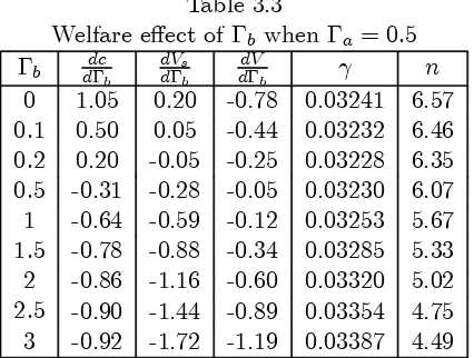
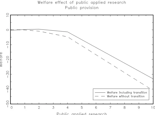
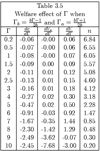
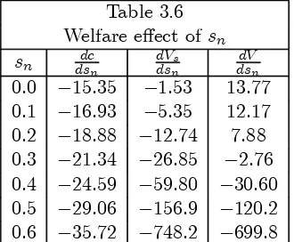
(10) 7 rameters used by developed countries. We …nd di¤erent e¤ects on growth and welfare and on the level of private research intensity induced by these policies. In particular, while direct research subsidies and publicly …nanced research have unambiguously positive e¤ects on growth, research performed at public institutions may damage economic growth. This is due to the crowding out of private research caused by public research when it competes with private …rms in the “patent race”. Another important feature of research is introduced in this chapter. Namely, the di¤erence between basic and applied research. In consonance with the literature on this topic, applied research is concerned with projects aimed at the obtention of an innovation with market applications and, thus, they will normally give rise to a patent. In contrast, basic research is devoted to projects whose outcomes do not initially have market applications though they add to the knowledge base and allow for the development of future projects with applied components. Both the public and the private sector will be allowed to perform both types of research. We will observe that the growth e¤ects of public research will be very di¤erent depending on whether it is oriented to applied or basic …elds. Namely, I …nd that while the e¤ect on growth of public basic research is unambiguously positive, the in‡uence of public applied research may be growth reducing due to the large negative impact of this type of intervention on private research. Finally, a welfare evaluation of all the policies considered suggests that welfare may be improved with research policy though an excessive or badly designed intervention may damage consumer welfare.. The process of technological change does not a¤ect all sectors uniformly. Innovative sectors gain productivity and pro…ts relative to the rest of the economy while non-.
(11) 8 innovative sectors see their technology become obsolete and their pro…ts shrink. There exists thus a distribution of productivities and pro…ts that may be a¤ected by the determinants of economic growth. How changes in these determinants may in‡uence this distribution is the object of the last chapter of the thesis. I …nd that when an economy is growing faster due to a larger productivity of research, or to a tax policy that stimulates capital accumulation, inequality will decrease. However, when faster growth is due to tax incentives to research in high technology sectors or to structural changes that allow a better absorption of spillovers, inequality among productive sectors will increase. Similarly, changes a¤ecting the distribution of productivities may also be associated with speci…c changes in the growth behavior of the economy. If the scope of technological spillovers is su¢ciently broad, a distribution with a larger mass of high-tech sectors will be associated with a higher growth rate. Nevertheless, a larger mass of research intensive sectors is not necessarily associated with faster growth when spillovers are technology speci…c or narrow in scope. In this case, the size of the leading group will not a¤ect the growth rate because the increased probability of innovation due to the larger mass of high-tech products is completely o¤set by the reduction in the marginal impact of an individual innovation..
(12) 9. Bibliography [1] Abramovitz, M. (1956) “Resource and output trends in the United States since 1870.” American Economic Review Papers and Proceedings 46, 5-23.. [2] Aghion, P. and P. Howitt (1998) “Endogenous growth theory” MIT Press.. [3] Aghion, P. and Howitt, P. (1992) “A model of growth through creative destruction” Econometrica 60, 323-351.. [4] Arrow, K. (1962) “The economic implications of learning-by-doing.” Review of Economic Studies 29(1), 155-173.. [5] Barro, R. (1990) “Government spending in a simple model of endogenous growth.” Journal of Political Economy 98(5), s103-s125.. [6] Cass, D. (1965) “Optimum growth in an aggregative model of capital accumulation.” Review of Economic Studies 32, 233-240.. [7] Grossman, G. and Helpman, E. (1991) “Trade, knowledge spillovers and growth.” European Economic Review 35, 517-526..
(13) 10 [8] Howitt, P. (1999) “Steady endogenous growth with population and R&D inputs growing” Journal of Political Economy 107(4), 715-730. [9] Howitt, P. and Aghion, P. (1998) “Capital accumulation and innovation as complementary factors in long-run growth” Journal of Economic Growth 3, 111-130. [10] Jones, C. (1995) “R&D-based models of economic growth.” Journal of Political Economy 103, 759-784. [11] Kendrick, J. (1956) “Productivity trends: Capital and labor.” Review of Economics and Statistics 38, 248-257. [12] Koopmans, T. (1965) “On the concept of optimal economic growth” The econometric approach to development planning, Amsterdam, North-Holland. [13] Ramsey, F. (1928) “A mathematical theory of saving.” Economic Journal 38, 543-559. [14] Romer, P. (1990) “Endogenous technological change” Journal of Political Economy 98(5), s71-s102. [15] Romer, P. (1986) “Increasing returns and long-run growth.” Journal of Political Economy 94(5), 1002-1037. [16] Schumpeter, J. (1942) “Capitalism, Socialism and Democracy”, New York. Harper: [17] Solow, R. (1957) “Technical change and the aggregate production function” Review of Economics and Statistics 39, 312-320..
(14) 11. Chapter 2. Financial Intermediation in a Model of Growth through Creative Destruction. 2.1. Introduction The renewed interest on growth and their determinants has pointed at the …nancial. structure as one of the key factors in the development of nations. This paper introduces a …nancial sector in one of the more recent models of growth, the one …rst presented in Howitt and Aghion (1998). This framework allows us to explicitly model how the R&D activity is …nanced by means of contracts designed to reduce the incidence of researcher’s moral hazard. As a consequence, the …nancial sector will have real e¤ects on the economy. Analyzing the interaction between …nancial and economic activity has been the.
(15) 12 aim of a rather proli…c literature. The …rst remarkable reference is the work of Schumpeter at the beginning of the twentieth century. He suggested that …nancial institutions are important for economic activity because they evaluate and …nance entrepreneurs in their research and development projects. Similarly, development economists like Gurley and Shaw (1955), Goldsmith (1969), and McKinnon (1973) defended the idea that …nancial development encourages growth because it increases the level of investment and improves its allocation. In addition, they argued that faster growing economies require higher amounts of …nancial services and that the richer the economy, the sooner it is able to pay for …nancial superstructures. Unfortunately, a lack of formal analysis is common to all these papers on development. This is probably because previous to the formulation of a rigorous framework on the relationship between …nance and growth it was necessary to develop further the theory of economic growth.. Neoclassical exogenous growth theory did not o¤er the appropriate frame of reference because …nancial variables could only have level e¤ects. The appearance of the …rst works on endogenous growth determined the starting point of the literature on growth and …nance. Classic references of this …rst line of research are Greenwood and Jovanovic (1990), Bencivenga and Smith (1991, 1993), Levine (1991, 1992) and Saint Paul (1992). They used the basic Ak framework combined with credit market models of …nancial intermediation. In these papers, …nancial markets are considered as institutions intended to provide services of risk pooling and collection of information about borrowers. They also facilitate the ‡ow of resources from savers to investors in the presence of market imperfections. Papers on this area introduce several devices to …ght against adverse selection, moral hazard or liquid-.
(16) 13 ity shocks in order to make intermediaries arise endogenously. The role of intermediation is thus, to reduce the ine¢ciency caused by these imperfections. Consequently, …nancial institutions promote growth because their activity implies a more e¢cient allocation of resources. With respect to the backward link from growth to …nance suggested by empirical evidence, they follow the basic argument of earlier work. Namely, that there exists a …xed component in the cost of …nancial services and that some limit of wealth must be trespassed before the establishment of a …nancial structure is a¤ordable.. New developments in the theory of economic growth have led to another line of research. Grossman and Helpman (1991b) and Romer (1990) suggested that economic growth comes mainly from the invention and development of new products rather than from the accumulation of physical or human capital. Recovering the Schumpeterian view of the role of …nancial institutions in economic activity, some authors tried to explain how …nancing of innovation can a¤ect the growth process. Good exponents of this literature are King and Levine (1993a), De la Fuente and Marín (1996) and Blackburn and Hung (1998). Using this new framework they introduce informational frictions in the credit market, providing a rationale for the appearance of intermediaries. King and Levine consider …nancial intermediaries that act as evaluators of prospective entrepreneurs and as providers of insurance for innovators. However they do not introduce incentive problems. This type of problems can arise because risk averse innovators will try to get full insurance. That is, they will try to get the same payment no matter whether they innovate or not. If this payment is positive, researchers do not have incentives to innovate, especially, if to innovate they must exert e¤ort. The papers by De la Fuente and Marín, and Blackburn and Hung take this.
(17) 14 moral hazard problem into account though from di¤erent perspectives. The …rst pair of authors provides banks with an imperfect monitoring technology that reveals the innovator’s level of e¤ort with a certain probability, while Blackburn and Hung use the costly state veri…cation paradigm, that is, that innovators have incentives to declare that they have not been successful so as to avoid payment. At some cost, investors can verify the result of the project. The common message of this group of papers is that …nancing of innovation is crucial for economic growth, and that the more e¢cient is the …nancial sector the faster the economy will grow. Concerning the feedback e¤ects of growth on …nance, these models provide a natural link without recurring to …xed costs assumptions. De la Fuente and Marín argue that growth causes changes in factor prices which increase the return to information gathering and hence favor …nancial intermediation activities. The above growth models used by the latter line of research ignore capital accumulation as a source of growth. Aghion and Howitt (1998) argue that they ignore capital accumulation because it is assumed that labor is the only input into research and that labor is inelastically supplied. Therefore, a rise in capital intensity will have two opposite e¤ects. On one hand, it will make payo¤s to innovation greater but on the other hand, it will increase labor’s productivity, making the input to research more expensive. These two e¤ects cancel each other out so that capital accumulation leaves innovative activity unaffected and thus, it cannot in‡uence long run growth.1 However, it is arguable that the only source of growth is innovation and, accordingly, Aghion and Howitt propose another model of creative destruction with capital accumulation. They assume that research is produced out of labor and intermediate inputs. In their model, both R&D activities and capital 1. For details see Aghion and Howitt (1998) pages 99-102..
(18) 15 accumulation determine growth and moreover, they are complementary. Growth cannot go on forever if there were no innovation because diminishing returns would reduce investment while without capital accumulation the rising cost of capital would choke o¤ innovation. This paper explicitly models the contractual relationship between the researcher and the provider of funds for the project in a model of endogenous technological change in the spirit of Howitt and Aghion (1998). Financial intermediaries are endowed with a monitoring technology that allows them to force researchers to exert a higher level of e¤ort than the one they would choose in the absence of monitoring. Hence, research productivity is determined in the credit market and thus, may be a¤ected by …nancial variables. In particular, the promotion of …nancial activities will enhance the economy’s growth performance. That is, subsidies to …nancial intermediation will increase R&D productivity moving the economy to a faster growing balanced growth path. In addition, a subsidy to …nancial intermediation may be more e¤ective than a direct subsidy to research. The latter policy induces a higher research intensity that rises the growth rate. However, the tax change reduces researchers’ incentives to exert e¤ort, which implies higher monitoring costs and a lower R&D productivity. This undercuts the positive growth e¤ects of the research subsidy to the point that for a high enough subsidy rate, the growth e¤ect can become negative. It is also shown that there exists a negative relationship between the equilibrium level of …nancial services and capital accumulation. The intuition for this comes from the fact that a policy that promotes …nancial activity will increase research productivity and thus, reduce the incentives to accumulate capital due to the business stealing e¤ect. The e¤ect of …nancial activity on research productivity causes two external e¤ects.
(19) 16 of opposite sign. On one hand, its positive e¤ect on the productivity of the research project will spillover to the other sectors of the economy and it will increase their productivity. On the other hand, the increase in R&D productivity will raise the arrival rate of innovations and consequently, the probability that an incumbent producer is replaced by the latest innovator. The higher probability of being replaced and thus, of losing the ‡ow of pro…ts, discourages capital accumulation. This is the so-called business stealing e¤ect, or creative destruction process. The interaction of these externalities makes the no-tax equilibrium level of …nancial services ine¢cient. Consequently, there exists a role for policies aimed at bringing the provision of …nancial services closer to its e¢cient level. The paper is divided in 6 sections. Section 2 presents the model, sections 3 and 4 study the steady state and the dynamics of the system respectively, section 5 performs the welfare analysis and section 6 concludes the paper.. 2.2. The model I consider a model of creative destruction with capital accumulation and tech-. nological spillovers.2 In the basic model without intermediation, capital accumulation and investment in R&D are the key variables for long run growth. In the present model however, they are not the only ones. This is due to the fact that research productivity is no longer an exogenous parameter. It will be determined by the amount of resources devoted to the …nancial sector of the economy. The availability of …nancial services increases the success probability of projects and, hence, the productivity of research. Thus, …nancial activities 2. The growth model is based on the work of Howitt and Aghion (1998)..
(20) 17 will also be relevant for the determination of long run growth.. 2.2.1. Consumers There is a representative consumer who maximizes the present value of utility. V (Ct ) =. Z. 1. ln(Ct )e¡½t dt:. (2.1). 0. I use the logarithmic functional form for simplicity. As usual Ct is consumption at date t and ½ is the rate of discount of consumption.. 2.2.2. Final good sector The consumption good is produced in a competitive market out of labor and. intermediate goods. Labor is represented by a continuous mass of individuals L; and it is assumed to be inelastically supplied. Intermediate goods are produced by a continuum of sectors of mass 1, being mit the supply of sector i at date t: The production function is a Cobb-Douglas with constant returns on intermediate goods and e¢ciency units of labor 1¡®. Yt = L. Z. 0. 1. Ait m®it di;. where Yt is …nal good production and Ait is the productivity coe¢cient of each sector. I assume equal factor intensities to simplify calculations.. 2.2.3. Intermediate goods The intermediate sector has a monopolistic structure. In order to become the. monopolist producer of an intermediate good, the entrepreneur has to buy the patent of.
(21) 18 the latest version of the product. This patent gives him the right to produce the good until an innovation occurs and the monopolist is displaced by the owner of the new technology. The only input in the production of intermediate goods is capital. In particular, it is assumed that Ait units of capital are needed to produce one unit of intermediate good i at date t: As we will see, this assumption is necessary in order to obtain stability. The evolution of each sector’s productivity coe¢cient; Ait is determined in the research sector. Capital is hired in a perfectly competitive market at the rental rate ³ t : Hence, the cost of one unit of intermediate good is Ait ³ t : On the other hand, the equilibrium price of the intermediate good, p(mit ) will be its marginal product p(mit ) = ®L1¡® Ait m®¡1 it ; where mit is production of intermediate good i at date t: Thus, the monopolist’s pro…t maximization problem is the following:. ¼ it = max[p(mit )mit ¡ Ait ³ t mit ] mit. s:t: p(mit ) = ®L1¡® Ait m®¡1 it ; from where we obtain the pro…t-maximizing supply and the ‡ow of pro…ts as. mit. µ. ®2 = L ³t. 1 ¶ 1¡®. ¼ it = ®(1 ¡ ®)L1¡® Ait m®it : Thanks to the assumption of equal factor intensity, supply of intermediate goods is equal in all sectors, mit = mt . Thus, the aggregate demand of capital is equal to Let At =. R1 0. R1 0. Ait mt di:. Ait di; be the aggregate productivity coe¢cient. Then, equilibrium in the capital.
(22) 19 market requires demand to equal supply. At mt = Kt ; or equivalently, the ‡ow of intermediate output must be equal to capital intensity kt ; mt =. Kt ´ kt : At. With this notation we can express the equilibrium rental rate in terms of capital intensity ³ t = ®2 L1¡® kt®¡1 :. 2.2.4. (2.2). Research sector Innovations are produced using the same technology of the …nal good. Hence,. it needs physical capital (embodied in the intermediate goods) apart from labor to be produced. Technology is assumed to be increasingly complex and hence further innovations will require higher investments. Accordingly, if Nt is the amount invested in research, the Poisson arrival rate of innovations will be ¸t nt ; where nt =. Nt Amax t. is the productivity. adjusted level of research and ¸t is research productivity: The total amount of investment in research is divided by Amax in order to take into account the e¤ect of increasing technological t is the leading edge coe¢cient that represents the aggregate state complexity since Amax t of knowledge. We approximate aggregate technological development by the productivity coe¢cient of the most advanced technology in the economy. When an innovation occurs, : The leading edge the productivity coe¢cient of that sector jumps discontinuously to Amax t coe¢cient grows gradually, at a rate that depends on the aggregate ‡ow of innovations. The m®t ; is the ‡ow of pro…ts to a monopolist who started producing at t, ® (1 ¡ ®) L1¡® Amax t.
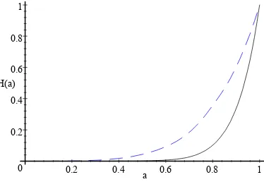
(23) 20 payo¤ to innovators if they succeed. Because this payment does not depend on the sector, the level of research will be the same across sectors and the aggregate ‡ow of innovations is thus ¸t nt : We will assume that Amax grows at a rate proportional to this aggregate ‡ow t of innovations A_ max t = ¾¸t nt ; Amax t. ¾ > 0:. It can be proved (see Appendix A) that the long-run cross-sectorial distribution of the relative productivity parameters, ait = 1. H(a) = a ¾ ;. Ait ; Amax t. is time invariant and equal to. 0 · a · 1:. (2.3). To simplify, it is assumed that the initial distribution of a is also H(a). Consider the arbitrage equation of the research sector. This equation establishes the equality between the expected value of an innovation and its cost at the margin. The value of an innovation at t; Vt ; must be the present value of the future ‡ow of pro…ts to the incumbent producer until a new technology displaces the monopolist. This ‡ow of pro…ts L1¡® kt® ; so the present value is given by is (1 ¡ ®)®Amax t Vt =. Z. t. 1. e¡. R¿ t. [rs +¸s ns ]ds. (1 ¡ ®)®Amax L1¡® k¿® d¿ : t. The expected marginal revenue of the innovation must equal its marginal cost. The cost of one unit of research in terms of output is 1. Therefore, since nt =. Nt ; Amax t. the cost of one unit. : I assume that there is a proportional tax on innovation that of research intensity is Amax t increases its cost.3 Thus, the marginal cost of increasing research intensity is (1 + ¿ n )Amax t 3. Perhaps, this is better understood if we consider a negative tax, i.e. a subsidy. The subsidy would reduce the cost of innovation..
(24) 21 units of output, where ¿ n is the tax to innovative activity. Hence, the research arbitrage condition may be written as 1 + ¿ n = ¸t. (1 ¡ ®)®L1¡® kt® : rt + ¸t nt. (2.4). Equation (2.4) gives the research intensity as a function of capital intensity and the endogenously determined arrival rate of innovations, ¸t . Thus, the equilibrium level of research is a function of capital intensity and, indirectly, of …nancial intensity.4. 2.2.5. Capital market Capital is used as a factor of production in the intermediate goods sector. We have. seen that equilibrium in the capital market requires the rental rate to satisfy equation (2.2). The owner of a unit of capital will obtain ³ t for it. This amount must be enough to cover the cost of capital. This includes the rate of interest (rt ), the depreciation rate (±), and the tax rate on capital accumulation (¿ k ). Hence, the capital market arbitrage equation is rt + ± + ¿ k = ®2 L1¡® kt®¡1 ;. (2.5). which establishes a decreasing relationship between the interest rate and capital intensity.. 2.2.6. Financing of research Financial intermediaries channel savings both for its use as capital in production. and to …nance research projects. I assume that each intermediary has access to deposits at the market determined rate of interest. There is no risk of bankruptcy because they hold a perfectly diversi…ed portfolio of production loans and research …nancing contracts. 4. The arrival rate of innovations, or R&D productivity, is positively related to monitoring intensity..
(25) 22 No imperfection is introduced in the provision of production loans. However, I will consider some degree of informational asymmetry in the design of research …nancing contracts. In particular, I assume that researchers have no funds to invest in the project and, therefore, they have to look for external …nance. The limited liability constraint implies that there will exist a potential problem of moral hazard on the part of the researcher. The funds needed for the project will be provided by intermediaries which are endowed with a monitoring technology that allows them to increase the e¤ort of the researcher. Moreover, I assume that the intensity with which the intermediary monitors the researcher determines the additional e¤ort that the former can force the latter to exert, as in Besanko and Kanatas (1993). It is assumed that there exists a one-to-one relationship between e¤ort and probability of success. Therefore, the monitoring services of the …nancial intermediaries determine R&D productivity. Consider a research project that requires an initial investment of one unit of output and that will yield a return v with probability ¸: Given the research sector outlined in the previous section, the return per unit of output invested, v; must be equal to. V Amax :. The. researcher obtains the funds from the intermediary and in exchange she will pay a …x amount p in case of success and nothing otherwise.5 The expected pro…ts for the researcher are given by. ¸(v ¡ p) ¡ D(¸); where D(¸) is the disutility caused by the e¤ort necessary to obtain a probability of success equal to ¸: We will assume that it takes the following form, which is borrowed from the 5. This is a consequence of the limited liability constraint..
(26) 23 work of Besanko and Kanatas (1993):. D(¸) =. ¸2 : 2¯. If the researcher received no monitoring at all, the level of e¤ort he would exert would be ¸0 = ¯(v ¡ p): This no-monitoring level of e¤ort is implementable at no cost for the intermediary. However, if the intermediary wishes to impose a higher level of e¤ort, he will have to face a cost which I assume increasing and convex in the di¤erence between the desired level of e¤ort and ¸0 .6 In particular, I assume that in order to obtain a success probability of ¸; the investment required is given by the following expression:. M(¸ ¡ ¸0 ) =. (¸ ¡ ¸0 )2 ; 2s. and therefore, the pro…ts of the intermediary can be written as. ¦I = ¸p ¡ (1 + ¿ f )M(¸ ¡ ¸0 ) ¡ 1; where ¿ f is a tax on the monitoring activities of intermediaries. Notice that imposing taxation on monitoring activities implies that we are assuming that the monitoring costs of the intermediary are observable. Thus we are considering moral hazard only on the part of the researcher. This di¤erent treatment can be justi…ed by the nature of the e¤ort that intermediaries and researchers do. The disutility caused to the researcher by this e¤ort is non-pecuniary while the monitoring e¤ort of banks can be measured in monetary units, a feature that makes it easier to observe, especially when we are talking about …nancial intermediaries, one of the most regulated sectors in developed economies. 6. See Besanko and Kanatas (1993) for details..
(27) 24 There exists a large number of intermediaries that compete in the provision of …nancial services. A researcher will choose one of them on the basis of his supply of …nancial services since it will determine the probability of success of her project. However, once the researcher chooses an intermediary to …nance her project, she will not be able to break this contract and ask another bank for …nance. This assumption can be justi…ed by the existence of switching costs or by the reluctancy of research …rms to reveal information about their project. In addition, the fact that once the choice is made the researcher cannot turn to another intermediary implies that the bank is placed in a position of power in its relationship with the researcher. In particular, for a given ¸; the intermediary will be able to impose the payment that maximizes his pro…ts, i.e. p(v; ¸) = v ¡. ¸ [¯(1 + ¿ f ) ¡ s] : ¯ 2 (1 + ¿ f ). (2.6). The fact that the intermediary is able to impose the payment that maximizes his pro…ts does not mean that the researcher is not going to gain with the contract. Indeed, the nature of the limited liability constraint implies that the researcher is always going to obtain a positive payment in expected terms.7 Notice also that this payment scheme implies a negative relationship between p and ¸: This is optimal for the intermediary because p is positively related to the monitoring cost of obtaining a given level of e¤ort. Additionally, if the researcher is subject to an intensive control, she will have to pay less to the intermediary while there is a higher probability that the project succeeds. This may compensate the 7. Recall that the payment is positive in case of success and zero in case of failure, which yields a positive payment in expected terms. In order to guarantee that the expected payment is positive we have to impose some restrictions on the parameters. In particular, we require s<. ¯(1 + ¿ f ) : 2.
(28) 25 researcher for the intensive monitoring. In fact, if the relationship between p and ¸ is given by (2.6), the expected pro…ts of the researcher become monotonically increasing in ¸: Hence, this contract makes monitoring desirable for the researcher, since it will reduce the share of the intermediary in the project’s return and increase the probability that the project succeeds. As a consequence, a researcher will choose the intermediary that o¤ers the highest level of monitoring services. Therefore, no ¸ that implies a positive amount of pro…ts will be an equilibrium since any intermediary can attract all the researchers by marginally increasing the degree of monitoring intensity and hence the probability of success. If the number of intermediaries is su¢ciently large to impede agreements that limit competition, in equilibrium bank pro…ts will be zero. Therefore, the equilibrium probability of success will be the highest value of ¸ that implies zero pro…ts. That is, it is the positive root of ¸p(v; ¸) ¡ (1 + ¿ f )M(¸ ¡ ¸0 (v; p(v; ¸))) ¡ 1 = 0 which yields a positive relationship between the productivity of research and the value of the project, as expressed by ~ ¸ = ¸(v):. 2.2.7. (2.7). Equilibrium Equations (2.4), (2.5) and (2.7) determine partial equilibrium in each market.. These equations can be combined in order to obtain the following equilibrium conditions for each market: (a) Research market equilibrium 1 + ¿ n = ¸t (vt ¡ p(vt ; ¸t )):. (2.8).
(29) 26 (b) Capital market equilibrium rt + ± + ¿ k = ®2 L1¡® kt®¡1 :. (2.9). (c) Credit market equilibrium ~ t ): ¸t = ¸(v. (2.10). Notice that the research arbitrage condition has been modi…ed to take into account the payment to the intermediary. Equations (2.6) and (2.8) imply the following equilibrium expression for ¸: ·. ¯ 2 (1 + ¿ f )(1 + ¿ n ) ¸= ¯(1 + ¿ f ) ¡ s. ¸ 12. :. (2.11). Hence, research productivity is time invariant and depends only upon the research and credit markets’ structural parameters. Using (2.11), equation (2.10) may be written in the following form:. vt =. ¸ ; © (¿ f ; ¿ n ). where. © (¿ f ; ¿ n ) =. 2¯ 2 (1 + ¿ f )(1 + ¿ n ) : (1 + ¿ n ) [2¯(1 + ¿ f ) ¡ s] + 2 [¯(1 + ¿ f ) ¡ s]. Thus, the system formed by equations (2.8), (2.9) and (2.10) can be reduced to the following system:8 ·. ¯ 2 (1 + ¿ f )(1 + ¿ n ) ¸= ¯(1 + ¿ f ) ¡ s 8. ¸ 12. :. Notice that in equation (2.12) we are just substituting vt by its expression in equilibrium..
(30) 27 ®(1 ¡ ®)L1¡® kt® ¸ = © (¿ f ; ¿ n ) rt + ¸nt. (2.12). rt + ± + ¿ k = ®2 L1¡® kt®¡1 ;. (2.13). which determines the equilibrium values of kt and nt : Notice also that from equations (2.12) and (2.13) one can obtain the equilibrium relationship between nt and kt as given by. nt = nd (kt ) =. © (¿ f ; ¿ n ) (1 ¡ ®)®L1¡® kt® ®2 L1¡® kt®¡1 ¡ ± ¡ ¿ k ¡ : 1 + ¿n ¸ ¸2. (2.14). With this equilibrium relationship the model can be reduced to a dynamic system of two di¤erential equations in capital and consumption. The law of motion of capital is given by. ¢. K t = Yt ¡ Ct ¡ Nt ¡ Et ¡ ±Kt ; where Et is the total amount of resources invested in monitoring. If M (¸ ¡ ¸0 ) is the monitoring cost per unit of output invested in research, then Et must equal M(¸ ¡ ¸0 )Nt : Notice that in equilibrium M(¸ ¡ ¸0 ) is a constant. Thus, in order to simplify, let us denote it by e = M(¸ ¡ ¸0 ) =. s(1+¿ n ) 2(1+¿ f )[¯ (1+¿ f )¡s]. so that Et will be equal to eNt :. The law of motion for consumption comes from utility maximization. ¢. C t = (rt ¡ ½)Ct: In order to obtain a system with steady state, express all variables in terms of e¢ciency.
(31) 28 units. 9. ¢. kt = L1¡® kt® ¡ ct ¡ (1 + ¾)(1 + e)nt ¡ (± + gt )kt. (2.15). ¢. ct = (rt ¡ ½ ¡ gt )ct ;. (2.16). and substitute the equilibrium expressions for rt ; gt and nt in equations (2.15) and (2.16) to express the system in terms of capital intensity and consumption per e¢ciency unit ¢. kt = L1¡® kt® ¡ ct ¡ (1 + ¾)(1 + e)nd (kt ) ¡ (± + g d (kt ))kt ¢. ct = (®2 L1¡® kt®¡1 ¡ ± ¡ ¿ k ¡ ½ ¡ g d (kt ))ct : where g d (kt ) = ¾¸nd (kt ): Due to the non-linearity of the system it must be linearized around the steady state in order to analyze the local dynamics. Accordingly, we will study the system at the steady state in the next section.. 2.3. Steady State Analysis In a steady state all variables grow at a constant rate. If we substitute the equi-. librium values mit = kt =. Kt At. in the aggregate production function, we obtain the usual. Cobb-Douglas functional form at the aggregate level Yt = (At L)1¡® Kt® : 9. Note that At =. Therefore,. Nt At. =. Z. 1. Ait di = Amax t. 0. (1+¾)Nt Amax t. Z. 1 0. = (1 + ¾) nt :. Ait di = Amax t Amax t. Z. 1 0. ah(a)da = Amax E(a) = t. Amax t : 1+¾.
(32) 29 This expression implies that the rate of growth of output will be that of the aggregate productivity coe¢cient and, given that At is proportional to the leading edge coe¢cient, the growth rate of the economy will be g = ¾¸n; where ¸ and n are constant and determined jointly with k through the equilibrium conditions of research, capital and credit markets.10 These conditions, evaluated at the steady state, are the following: ¸ ®(1 ¡ ®)L1¡® k ® = © ½ + (1 + ¾)¸n ½ + ¾¸n + ± + ¿ k = ®2 L1¡® k®¡1 ·. ¯ 2 (1 + ¿ f )(1 + ¿ n ) ¸= ¯(1 + ¿ f ) ¡ s. ¸ 12. (2.17). ;. from where we obtain n=. ©(¿ f ; ¿ n ) ®(1 ¡ ®)L1¡® k® ½ ¡ ; 2 (1 + ¾) (1 + ¾)¸ ¸. (2.18). and the equation that implicitly determines the steady state value of k; which is the result of plugging (2.18) into (2.17) F (k) =. ©(¿ f ; ¿ n ) ¾ ½ + ®(1 ¡ ®)L1¡® k ® + ± + ¿ k ¡ ®2 L1¡® k ®¡1 = 0: (2.19) (1 + ¾) ¸ (1 + ¾). The steady state growth rate can be expressed in terms of capital intensity using equation (2.17) to obtain g = ®2 L1¡® k®¡1 ¡ ½ ¡ ± ¡ ¿ k : 10. Variables without time suscript denote steady state values..
(33) 30 The use of implicit di¤erentiation allows us to analyze the e¤ect on k of parameter changes, and to obtain the following comparative statics results:. Proposition 1 The steady state growth rate increases with subsidies to capital accumulation and to …nancial activity. The growth rate is decreasing (increasing) in ¿ n when ³ ´ s s ¿ n > ¡ 2¯(1+¿ < ¡ ¿ n 2¯(1+¿ f )¡s : f )¡s Proof. See Appendix.. Proposition 2 The steady state growth rate is increasing in ¾ (the size of innovations); decreasing in ½ and ± and increasing in s (the scale parameter of the monitoring costs) and ¯ (the scale parameter of the disutility of e¤ort).. Proof. See Appendix.. Proposition 1 establishes a marginal positive relation between …nancial activity and growth. This relation may be understood because a subsidy to …nancial activity (or equivalently a reduction in ¿ f ) implies a lower monitoring cost. Thus, monitoring intensity increases. Accordingly, the positive growth e¤ect of this policy is due to the externality that …nancial activity causes on the accumulation of public knowledge. Promoting …nancial activity is equivalent to increase the productivity of R&D and thus, to make a better use of the resources allocated to research. The result obtained for the growth e¤ects of research subsidies re‡ects the moral hazard problem of R&D. The smaller cost of research represents an increase of the expected return for researchers that does not depend on the e¤ort they exert. It can be shown that a.
(34) 31 lower ¿ n reduces the no monitoring level of e¤ort.11 This implies a higher monitoring cost and, thus, ¸ falls. Therefore, even though we expect a positive e¤ect on research intensity, the R&D productivity reduction may be enough to cause a negative e¤ect on the growth rate. Aghion and Howitt (1998) argue that capital accumulation and innovation are complementary factors for long run growth. To illustrate this assertion, they reduce the capital tax, a measure that directly a¤ects the capital market, and study the reaction of the economy. The reduction of the cost of capital rises the equilibrium value of capital intensity making the ‡ow of pro…ts accruing to a successful innovator grow. Consequently, investment in the research sector will increase. Thus a policy that directly favors capital accumulation also incentives innovation and economic growth. The same argument can be applied in the present model. Therefore, innovation and capital accumulation continue being complementary factors for long run growth. Furthermore, this policy has no negative e¤ects either on ¸0 or on ¸: Thus, a subsidy to capital accumulation may be preferable in terms of growth to a direct subsidy to research. We can perform the same experiment on …nancial activity. Thus, let us reduce the …nancial tax. The lower monitoring cost stimulates the production of …nancial services, inducing a rise in the arrival rate of innovations and, consequently, a larger rate of creative destruction. This discourages capital investment because the incumbent monopolist faces a larger probability of being replaced. Thus, the e¤ect on capital accumulation is negative. 11. The equilibrium expression for ¸0 is given by ¸0 =. Thus, the result follows immediately.. ·. (1 + ¿ n ) [¯ (1 + ¿ f ) ¡ s] (1 + ¿ f ). ¸1 2. :. (2.20).
(35) 32 That is, a policy that incentives …nancial activity will make the economy grow faster even though it will discourage capital investment. Therefore, capital and …nancial intensity should be considered substitutive factors for long run growth. Notice that this negative e¤ect of research …nancing on capital accumulation undercuts the growth e¤ects of intermediation promoting policies. At the no-tax equilibrium a marginal reduction of any of the three taxes would increase the growth rate. In order to identify the most e¤ective policy, the tax changes are made equivalent in terms of the amount of resources generated for the government budget. The budget constraint of the government is given by ¿ n Nt + ¿ k Kt + ¿ f Et = T; where T is the lump-sum transference or tax used to balance the budget when we introduce a policy change. In order to make two policy changes equivalent, the change induced on T must be the same. Therefore, to compare the growth e¤ects of ¿ k ; ¿ f and ¿ n ; we must compare the following expressions: ¯ dg 1 dg d¿ k dg ¯¯ = = ¯ dT dT =Kt d¿ k d¿ k dT d¿ k Kt ¯ dg ¯¯ dg 1 dg d¿ f = = ¯ dT dT =Et d¿ f d¿ f dT d¿ f Et. ¯ dg ¯¯ dg d¿ n dg 1 = ; = dT ¯dT =Nt d¿ n d¿ n dT d¿ n Nt. all evaluated at ¿ f = ¿ k = ¿ n = 0: This allows us to establish the following propositions: Proposition 3 At the no-tax equilibrium, the growth e¤ect of ¿ f is stronger than the growth e¤ect of ¿ n ; i.e.,. dg 1 d¿ f Et. <. dg 1 d¿ n Nt :.
(36) 33 Proof. See Appendix.. Proposition 4 At the no-tax equilibrium, the growth e¤ect of ¿ f is stronger than the growth e¤ect of ¿ k ; i.e.. dg 1 d¿ f Et. <. dg 1 d¿ k Kt ;. whenever. ® (1 ¡ ®) L1¡® k® <. ¸ 2 [¯ ¡ s] ½: © s. (2.21). Proof. See Appendix.. Proposition 3 implies that, at the no-tax equilibrium, subsidizing the …nancial sector will be more growth promoting than directly subsidizing research. Similarly, Proposition 4 implies that the …nancial tax may have larger e¤ects on growth than the capital tax. Therefore, there exist situations in which subsidizing …nancial activity is the most e¤ective policy in order to improve the growth performance of the economy. Notice that in the case of Proposition 4, condition (2.21) is expressed in terms of k which is an endogenous variable. Consequently, it could happen that the condition is never satis…ed. However, by means of calibration, it is relatively easy to …nd sets of parameters for which the condition is satis…ed. Notice also that the e¤ectiveness of the …nancial tax depends upon s; the scale parameter for monitoring costs. A small s means a large monitoring cost and a low monitoring intensity, e. Therefore, the lower the s, the smaller the relative amount of resources allocated to …nancial services in equilibrium and the stronger the marginal e¤ect we can induce on monitoring intensity. To sum up, this result proposes the use of subsidies or tax cuts to …nancial activity as an alternative instrument to promote innovation without the moral hazard problems of direct research subsidies..
(37) 34. 2.4. Dynamics After analyzing the behavior of the economy at its long run equilibrium, the system. can now be linearized so as to study the dynamics of the model around the steady state. Recall that the system is formed by the following equations: ¢. kt = L1¡® kt® ¡ ct ¡ (1 + ¾)(1 + e)nd (kt ) ¡ (± + g d (kt ))kt ¢. ct = (®2 L1¡® kt®¡1 ¡ ± ¡ ¿ k ¡ ½ ¡ g d (kt ))ct : The linearized system is obtained computing the Jacobian of the system and evaluating it at the steady state. In order to simplify notation let us express the system as follows ¢. k t = '(kt ; ct ; ¿ k ; ¿ f ; ¿ n ) ¢. ct = Á(kt ; ct ; ¿ k ; ¿ f ; ¿ n ): Then the derivatives needed are the following: 'k (k; c) = ®L1¡® k®¡1 ¡ (1 + ¾)(1 + e)nd0 (kt ) ¡ (± + g) ¡ k(gd0 (k)) 'c (k; c) = ¡1 Ák (k; c) = c(¡®2 (1 ¡ ®)L1¡® k®¡2 ¡ g 0d (k)) Ác (k; c) = 0: With this notation the linearized system will be ¢. kt = 'k (k; c) (kt ¡ k) ¡ (ct ¡ c) ¢. ct = Ák (k; c) (kt ¡ k): The determinant of the matrix of the system is equal to the function Ák (k; c) evaluated at the steady state, which can be proved to be negative. Therefore the system presents local.
(38) 35 saddle path stability. For future reference, let ¸1 be the negative eigenvalue and ¸2 the positive one.. 2.5. Welfare analysis Now that we have characterized the dynamics of the system we can analyze the. welfare implications of changes in tax parameters. From equation (2.1) we can express utility at the steady state in terms of the stationary level of consumption and the long-run growth rate. Vs (c; g) =. Z. 1. ln(cAt )e¡½t dt =. 0. g ln(cA0 ) + 2: ½ ½. The change in steady state welfare is a combination of the change in steady state consumption and the change in steady state growth @Vs (c; g) 1 @c 1 @g = + 2 @¿ i ½c @¿ i ½ @¿ i. for i = k; f; n:. (2.22). This measure of welfare is valid to compare two situations of long run equilibrium. However, it does not consider the periods of transition during which the economy moves from one equilibrium to another. In order to re‡ect the transition we must analyze the e¤ect on lifetime utility. Rewrite equation (2.1) to obtain the following expression for lifetime utility as a function of the di¤erent tax rates (¿ i where i = k; f; n:): ln(A0 ) V (¿ i ) = + ½. Z. 0. 1 ·Z t 0. ¸ Z ¡½t gs (¿ i )ds e dt +. 1. ln(ct (¿ i ))e¡½t dt. 0. where gt (¿ i ) and ct (¿ i ) are the time paths of the growth rate and the level of consumption per e¢ciency unit after a change in one of the tax parameters. The e¤ect on utility will.
(39) 36 thus be given by the e¤ects on the paths of growth and consumption. I will obtain …rst the e¤ect on the paths of consumption and capital intensity and then use the latter to get the e¤ect on the path of the growth rate. Let c = p(k; ¿ i ) be the saddle path of the system which can be interpreted as the graph of a policy function relating consumption and capital. Then, we know that its slope pk ; is positive and equal to. Ák ¸1 :. Substituting the policy function into the law of motion. of k; the equilibrium dynamics of the system can be characterized by a single di¤erential equation which describes the evolution of the state variable along the stable manifold. k_ = '(k; c) = '(k; p(k; ¿ i )) = ª(k; ¿ i ): The solution to this equation, kt (¿ i ), gives the equilibrium value of k as a function of time and the tax parameter: Using kt (¿ i ) in the policy function we would obtain the time path of c ct (¿ i ) = p(kt (¿ i ); ¿ i ): To calculate the change in welfare we need the derivative of the whole time path of c with respect to ¿ i dct (¿ i ) dkt (¿ i ) = pk + p¿ i ; d¿ i d¿ i. (2.23). where p¿ i is the derivative of the policy function with respect to the tax or graphically, the shift in the saddle path caused by the policy change. In order to compute. dkt (¿ i ) d¿ i ;. notice that kt (¿ i ) = k(t; ¿ i ) must satisfy identically. the original equation _ ¿ i ) ´ ' (p(k(t; ¿ i ); ¿ i ); k(t; ¿ i ); ¿ i ) ; k(t;.
(40) 37 di¤erentiate both sides with respect to ¿ i dk¿ i = ['c pk + 'k ] k¿ i + 'c p¿ i + '¿ i : k_ ¿ i = dt Hence k¿ i satis…es a linear di¤erential equation. Moreover, when we start from a steady state, the coe¢cients of this equation are constant and we can write k_ ¿ i = ¸1 k¿ i ¡ p¿ i + '¿ i : The general solution is given by. k¿ i (t) = exp (¸1 t) k¿ i (0) + (1 ¡ exp (¸1 t))k¿ i (1): Since k is a predetermined variable, the change at the date of the policy change k¿ i (0) must be zero. The long run e¤ect, k¿ i (1) = limt!1 k¿ i (t); is in fact the derivative of the steady state value of k with respect to the tax parameter, and can be expressed as. k¿ i (1) =. p¿ i ¡ '¿ i : ¸1. The equilibrium time path of the derivative of k with respect to ¿ i is thus given by ¸ p¿ i ¡ '¿ i ; k¿ i (t) = (1 ¡ exp(¸1 t)) ¸1 ·. that is, k will gradually reach its new steady state value at a rate equal to the negative eigenvalue. Substitute now in equation (2.23) to obtain the …nal expression for the derivative of the time path of consumption with respect to the tax parameter ¸ · p¿ i ¡ '¿ i dct (¿ i ) + p¿ i : = pk (1 ¡ exp(¸1 t)) d¿ i ¸1.
(41) 38 As before, we can identify the immediate change and the long run e¤ect dc0 (¿ i ) d¿ i dc1 (¿ i ) d¿ i. = p¿ i ; · ¸ p¿ i ¡ '¿ i + p¿ i ; = pk ¸1. where the …rst represents the necessary jump of consumption to get on the new saddle path and the second is the e¤ect on the steady state value of consumption. Thus, consumption will initially jump to the new saddle path and then it will approach its new steady state value at a rate equal to ¸1 : The derivative of the growth rate and consumption per e¢ciency unit at date t are given by dgt (¿ i ) d¿ i dct (¿ i ) d¿ i. = =. dg d (k) @k @gd (k) + (1 ¡ exp(¸1 t)) dk @¿ i @¿ i @c @k ¡ pk exp(¸1 t) : @¿ i @¿ i. (2.24) (2.25). Notice that the derivatives of g d are evaluated at the steady state because we consider the stationary equilibrium as the situation before the tax change. Expressions (2.24) and (2.25) allow us to write the change in welfare as follows: 3 2 (1¡®)³ ½¡¸1 dg d (k) + @V (¿ i ) @Vs (¿ i ) 4 ½ dk k 5 @k : = + (2.26) @¿ i @¿ i ¸1 (½ ¡ ¸1 ) @¿ i. Equations (2.22) and (2.26) give the general expressions for the e¤ect of the three taxes on the di¤erent measures of welfare. Let us see now the speci…c results for each policy.. 2.5.1. Tax on capital The e¤ect on welfare of the capital tax is given by @Vs (c; g) 1 @c 1 @g = + @¿ k ½c @¿ k ½2 @¿ k.
(42) 39 2 3 (1¡®)³ ½¡¸1 dgd (k) + @V (c; g) @Vs (c; g) 4 ½ dk k 5 @k ; = + @¿ k @¿ k ¸1 (½ ¡ ¸1 ) @¿ k. (2.27). where the …rst expression represents the e¤ect on welfare if the transition is excluded. Both the expression in square brackets in equation (2.27) and. @k @¿ k. are negative. Therefore, the. e¤ect on welfare using the second measure will always be larger than the e¤ect if we use the …rst measure. Proposition 1 shows that. @g @¿ k. is negative. However, the e¤ect on consumption is. ambiguous. The derivative of consumption with respect to the capital tax is given by k @c = © ¾ @¿ k 1 + ¸ 1+¾ k. µ ¶ 1 (1 + e)© ½ + ¿k © ¾ ¡ + ¡ + k : ® (1 ¡ ®) ³ ¸ 1+¾ ¸2. The functional form of this derivative implies that for large enough values of steady state capital intensity; the derivative will be positive while it may be negative for smaller values of k: Since the relationship between k and the capital tax is negative, this suggests that for negative or small values of ¿ k we might expect a positive e¤ect on consumption while for large values of the tax,. @c @¿ k. may become negative. Therefore, we may roughly represent the. relationship between consumption and the capital tax as an inverted U-shaped curve whose maximum shifts right or left depending on the structural characteristics of the economy. In summary, there may exist a consumption maximizing value of ¿ k but whether it is a subsidy or a tax depends upon the economy considered. These results can also be applied to the relationship between welfare and this tax. I have calibrated the model for a usually accepted set of parameters obtaining that in every case, the welfare maximizing rate of this policy instrument was a subsidy.12 Consequently, in economies with a positive capital tax 12 The set of parameters used includes ½ = 0:02; ± = 0:05; ¾ = ln(1:1) and L = 1: The values of ¯ and s were chosen so that the resulting steady state values of the growth rate and the probability of success lay in a reasonable interval. The computer program used for calibration is available upon request..
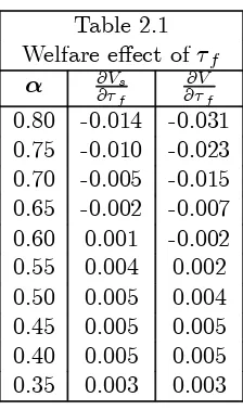
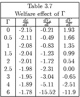
(43) 40 rate, a tax reduction will generally cause a welfare improvement.. 2.5.2. Tax on …nancial services The welfare derivatives for the …nancial tax are @Vs (c; g) 1 @c 1 @g = + 2 @¿ f ½c @¿ f ½ @¿ f. @V (c; g) @Vs (c; g) = + @¿ f @¿ f and given that. @k @¿ f. 2. ½¡¸1 dg d (k) dk 4 ½. +. (1¡®)³ k. ¸1 (½ ¡ ¸1 ). 3. 5 @k ; @¿ f. is positive, the e¤ect on welfare of this tax will always be smaller if we. consider the transition. As before, we know that the derivative of the growth rate with respect to this tax is negative. The e¤ect on consumption is given by @c @¿ f. ¶ µ @k 1 + ® (1 + e)© ½ + ¿k ¡ + = (1 ¡ ®) ³ + @¿ f ® (1 ¡ ®) ³ ¸2 · ¸ · ¸ @ © (1 + e) @ 1+e 1¡® ® + ¡ ® (1 ¡ ®) L k +½ : @¿ f @¿ f ¸ ¸2. (2.28). In order to simplify the analysis, the range of values of the tax parameters is restricted so that we can give an unambiguous sign to this derivative. To this end, we will not consider values of the capital tax rate below ¡½ nor subsidy rates to the research sector above 57 : Under these assumptions, we can establish the following proposition:. Proposition 5 If ¿ k > ¡½ and ¿ n > ¡ 57 ; the derivative of steady state consumption per e¢ciency unit with respect to the …nancial tax is positive.. Proof. See Appendix.
(44) 41 Consequently, a marginal change in the …nancial tax will cause opposite e¤ects on growth and consumption, depending the …nal change in welfare on which e¤ect dominates. Obviously, the value of the discount rate is determinant for the sign of derivative will be positive whenever. @c @¿ f. @Vs (c;g) @¿ f :. This. @g + ½c @¿ is positive. A small ½ means that consumers f. weight more heavily the growth e¤ect of the tax. Thus, if ½ is small enough, welfare will increase with reductions of the …nancial tax. Notice also that for a given discount rate, increases in ¿ f make steady state consumption per e¢ciency unit grow. Therefore, we may expect positive e¤ects on welfare for low values of the tax though they may disappear as the tax rate increases. Hence, we also …nd the inverted U-shaped curve representing the relationship between welfare and the …nancial tax. A calibration of the model gives a rough idea of how can …nancial policies improve welfare. At the no tax equilibrium and for the same set of parameters used before, I obtain the following results:. Table 2.1 Welfare e¤ect of ¿ f @Vs @V ® @¿ f @¿ f 0.80 -0.014 -0.031 0.75 -0.010 -0.023 0.70 -0.005 -0.015 0.65 -0.002 -0.007 0.60 0.001 -0.002 0.55 0.004 0.002 0.50 0.005 0.004 0.45 0.005 0.005 0.40 0.005 0.005 0.35 0.003 0.003 A negative sign of the welfare derivative means that the optimal policy is to reduce the …nancial tax. Conversely, a positive entry implies that the optimal policy is a.
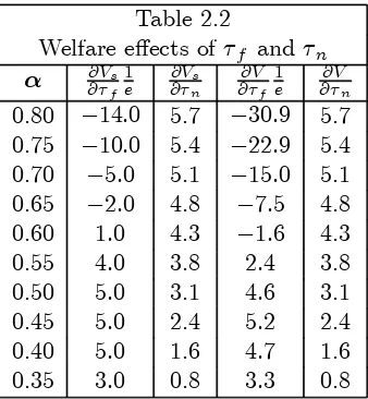
(45) 42 tax increase. This calibration suggests that …nancial services will be underprovided in a relatively capital intensive economy while in less capital intensive economies, a reduction of its provision could increase welfare. Recall that the …nancial sector has real e¤ects on the economy only because it can modify the productivity of research. A high ® means a relatively high equilibrium value of k which in turn implies a high research intensity. Therefore, a policy that favors monitoring and thus, increases the productivity of research, will have larger growth e¤ects in an economy with a relatively higher research intensity. This larger growth e¤ect will be able to compensate for the reduction in steady state consumption per e¢ciency unit. On the contrary, if ® is small, so is equilibrium research intensity and thus, the higher productivity in this case will not be able to induce a large enough increase in the growth rate.. 2.5.3. Tax on research activity The welfare derivatives for the research tax are. @Vs (c; g) 1 @c 1 @g = + 2 @¿ n ½c @¿ n ½ @¿ n. @V (c; g) @Vs (c; g) = + @¿ n @¿ n. 2. ½¡¸1 dg d (k) dk 4 ½. and as with the …nancial tax, the fact that. +. (1¡®)³ k. ¸1 (½ ¡ ¸1 ). @k @¿ n. 3. 5 @k ; @¿ n. is positive makes the e¤ect on welfare of. this tax smaller if we consider the transition. The derivative of steady state consumption per e¢ciency unit is given by the.
Figure
+7
Documento similar
To perform excellent research and technological developments in astrophysics, securing the appropriate training of graduate students, young researchers and
Previous articles have focused multiples valuation research on the selection of a peer group, establishing that firms in the same industry are expected to have similar
Accordingly, the increase in government spending (that in this case is equivalent to an increase of the budget deficit) will induce a direct (through its purchases) and
The coefficient jβ, is the measure of the degree of dynamic increasing returns in the industry, whereas the coefficient jα is the measure of all those influences on technical
49. The RCGP recommends that there is increased investment in research and development and funds to support primary care mental health services to increase education and training
Government policy varies between nations and this guidance sets out the need for balanced decision-making about ways of working, and the ongoing safety considerations
The Carlos III Institute of Health is the Public Research Organization (OPI) that promotes, manages and evaluates and finances biomedical research in Spain through the
This research aims to contribute to the debate on online and offline participation in the free culture movement in Spain. Additionally, we propose to address the following
